The Active Element Machine Michael Stephen Fiske
Abstract We present a new computing machine, called an active element machine (AEM), and the AEM programming language. This computing model is motivated by the positive aspects of dendritic integration, inspired by biology, and traditional programming languages based on the register machine. Distinct from the traditional register machine, the fundamental computing elements – active elements – compute simultaneously. Distinct from traditional programming languages, all active element commands have an explicit reference to time. These attributes make the AEM an inherently parallel machine and enable the AEM to change its architecture (program) as it is executing its program.
1 Introduction We present a new computing machine called an active element machine (AEM) and the active element machine programming language. This computing model is motivated by the positive aspects of dendritic integration, inspired by biology, and traditional programming languages based on the register machine. Distinct from the traditional register machine, the fundamental computing elements – active elements – compute simultaneously. Distinct from traditional programming languages, all active element commands have an explicit reference to time. These attributes make the AEM an inherently parallel machine and enable the AEM to change its architecture (program) as it is executing its program.
Michael Stephen Fiske Aemea Institute, San Francisco, CA, 94129. e-mail:
[email protected] The original publication is available at http://www.springerlink.com.
1
2
Michael Stephen Fiske
1.1 Wilfrid Rall’s Models of Dendritic Integration Wilfrid Rall’s research [36] in neurophysiology influenced the development of the active element machine – in particular, his work on dendritic integration and how this contributes to computation. Rall’s mathematical models are thorough and complicated; Rall modelled the non-linearities of the neuron and much of his work focussed on dendrites. Our goal was to capture the critical computational properties of dendritic integration that use its computational power while keeping the mathematics as simple as possible. Another goal was to assure that the mathematics and computing mechanism were simple enough to implement in silicon and other kinds of hardware ([18], [19]). Our third goal was to make the machine and language simple enough to design AEM programs implicitly, explicitly or both. An AEM program may be designed implicitly using evolutionary methods. An explicit AEM program is written by one or more persons. Early and current neural network models [26], [32] are complicated to program or do not have a simple programming language for designing the network. For the above reasons, implicit and explicit programmability were important criteria that influenced the design of the active element machine.
1.2 Register Machine Computation Another part of this development comes from the formal model of the Turing machine [46] and the subsequent von Neumann architecture. (This section contains some rhetorical content as a means to motivate new notions.) Today’s computers do not conceptually work much differently than these early models. Perhaps, the biggest difference is that today’s computers are much faster. In the current notion of an algorithm, the relevant concepts of the Turing computing model (see [46] and definitions 14, 15, 16, 17) are: • There are a finite number of alphabet symbols A = {a1 , . . . , an } read and written to a tape. • There are a finite number of machine states Q = {q1 , . . . , qm }. • The Turing program η is a finite set of rules that stays fixed: The rules do not change as the program executes. • The execution of one rule represents a computational step. During this computational step, one of the rules is selected, based on the current alphabet symbol pointed to by the tape head and the current machine state. The output of the rule specifies that a new alphabet symbol or the same symbol is written to the tape, the machine moves to a new state or stays in the current state and that the tape head moves one square to the left or right. • Computational steps are executed sequentially with no explicit reference to time.
The Active Element Machine
3
In light of the above, it seems natural for the Turing machine to lead to the register machine (see [1], [34], [45]). In the register machine, a program is a finite number of instructions that are executed in a linear sequence. Further, the contents of a register is changed in one computational step, which is analogous to writing a new symbol on the tape during one computational step of the Turing machine. In the register machine, there is also no explicit reference to an absolute or relative time. Furthermore, usually one register machine instruction is executed at a time, which creates a computational bottleneck.
1.3 Explicit Representation of Time The register machine is a programmable machine but the program is fixed during program execution. There is also no notion of explicit time in the register machine model, only the order in which instructions are executed. Rall’s research does not address programmability and has no notion of commands. His models used time, dendritic integration and adaptability of the synapses. The active element machine explicitly represents time in the machine commands which enables the following useful properties. • Parallel algorithms can be implemented in a natural way, since each active element performs computation and all of them simultaneously compute. • Explicit time in the active element commands enhances control over the active element machine computation because the synchronization of computation among different groups of active elements can be coordinated. This coordination helps avoid race conditions that can occur in the standard programming languages that implement concurrent processes. • The machine can change its own architecture (program) with the Meta command while it is executing. • The Meta command enables the active element machine’s complexity to increase over time. In [31], Edward Lee proposes using explicit time in a computing model and computing applications: This paper argues that to realize its full potential, the core abstractions of computing need to be rethought to incorporate essential properties of the physical systems, most particularly the passage of time. It makes a case that the solution cannot be simply overlaid on existing abstractions, . . . . The emphasis needs to be on repeatable behavior rather than on performance optimization.
4
Michael Stephen Fiske
1.4 Summary Overall, we introduce the active element machine and a programming language that can be used to explicitly or implicitly program the machine. We show that any register machine can be computed by an active element machine. Using randomness in the environment, time and the Meta command, we show how to construct an active element machine that corresponds to an arbitrary real number in [0, 1]. Building upon this example, this AEM is extended so that it can recognize an arbitrary language L ⊆ {0, 1}∗ . Finally, we demonstrate an example of an active element machine that finds the Ramsey number r(3, 3) ([22], [37]), illustrating how parallel AEM algorithms and time in the commands compute an NP-hard problem ([10], [12], [21]).
2 Machine Architecture An active element machine is composed of computational primitives called active elements. There are three kinds of active elements: Input, Computational and Output active elements. Input active elements process information received from the environment or another active element machine. Computational active elements receive messages from the input active elements and other computational active elements firing activity and transmit new messages to computational and output active elements. The output active elements receive messages from the input and computational active elements firing activity. The firing activity of the output active elements represents the output of the active element machine. Every active element is an active element in the sense that each one can receive and transmit messages simultaneously. Each active element receives messages, formally called pulses, from other active elements and itself and transmits messages to other active elements and itself. If the messages received by active element, Ei , at the same time sum to a value greater than the threshold, then active element Ei fires. When an active element Ei fires, it sends messages to other active elements. Let Z denote the integers. We define the extended integers as Z = {m + kdT : m, k ∈ Z and dT is a fixed infinitesimal}. For more on infinitesimals, see [39] and [25]. Definition 1. Machine Architecture Γ , Ω , and ∆ are index sets that index the input, computational, and output active elements, respectively. Depending on the machine architecture, the intersections Γ ∩ Ω and Ω ∩ ∆ can be empty or non-empty. A machine architecture, denoted as M (I , E , O), consists of a collection of input active elements, denoted as I = {Ei : i ∈ Γ }; a collection of computational active elements E = {Ei : i ∈ Ω }; and a collection of output active elements O = {Ei : i ∈ ∆ }. Each computational and output active element, Ei , has the following components and properties:
The Active Element Machine
5
• A threshold θi • A refractory period ri where ri > 0. • A collection of pulse amplitudes {Aki : k ∈ Γ ∪ Ω }. • A collection of transmission times {τki : k ∈ Γ ∪ Ω }, where τki > 0 for all k ∈ Γ ∪Ω. • A function of time, Ψi (t), representing the time active element Ei last fired. Ψi (t) = sup{s : s < t and gi (s) = 1}, where gi (s) is the output function of active element Ei and is defined below. The sup is the least upper bound. • A binary output function, gi (t), representing whether active element Ei fires at time t. The value of gi (t) = 1 if ∑ Aki (t) > θi where the sum ranges over all k ∈ Γ ∪ Ω and t ≥ Ψi (t) + ri . In all other cases, gi (t) = 0. For example, gi (t) = 0, if t < Ψi (t) + ri . • A set of firing times of active element Ek within active element Ei ’s integrating window, Wki (t) = {s : active element Ek fired at time s and 0 ≤ t − s − τki < ωki }. Let |Wki (t)| denote the number of elements in the set Wki (t). If Wki (t) = 0, / then |Wki (t)| = 0. • A collection of input functions, {φki : k ∈ Γ ∪ Ω }, each a function of time, and each representing pulses coming from computational active elements, and input active elements. The value of the input function is computed as φki (t) = |Wki (t)|Aki (t). • The refractory periods, transmission times and pulse widths are positive integers; and pulse amplitudes and thresholds are integers. The time t – that these parameters are a function of i.e. θi (t), ri (t), Aki (t), ωki (t), τki (t) – is an element of the extended integers Z. Input active elements that are not computational active elements have the same characteristics as computational active elements, except they have no inputs φki coming from active elements in this machine. In other words, they don’t receive pulses from active elements in this machine. Input active elements are assumed to be externally firable. An external source such as the environment or an output active element from another distinct machine M (I 0 , E 0 , O 0 ) can cause an input active element to fire. The input active element can fire at any time as long as the current time minus the time the input active element last fired is greater than or equal to the input active element’s refractory period. An active element, Ei , can be an input active element and a computational active element. Similarly, an active element can be an output active element and a computational active element. Alternatively, when an output active element, Ei , is not a computational active element, where i ∈ ∆ − Ω , then Ei does not send pulses to active elements in this machine.
6
Michael Stephen Fiske
Example 1. Overlapping Pulses with Different Firing Times Consider the four element machine where X, Y , and Z are input active elements and B is a computational active element. The parameters of the elements and their connections are shown in tables 1 and 2. Table 1 Element Parameter Values Element X Y Z B
Threshold
Refractory
Firing Times
10
1 1 1 2
4 1 2 5
No thresholds are shown for X, Y , and Z since they are input elements. Table 2 Connection Parameter Values Connection
From
To
Amplitude
Width
Transmission Time
XB YB ZB
X Y Z
B B B
3 4 4
4 2 2
1 3 2
Input elements X, Y , and Z are externally fired at times 4, 1 and 2, respectively. At time t = 3, pulses created by Y and Z are travelling to B but have not yet arrived. B does not fire. At time t = 4, pulses created by Y and Z arrive at B. The input to B is AY B (4) + AZB (4) = 8 which does not exceed B’s threshold. B does not fire. At time t = 5, pulses created by Y and Z are still at B because their pulse widths are 2. Also the pulse from X arrives. The input to B is AXB (5) + AY B (5) + AZB (5) = 11 which exceeds B’s threshold. B fires at time t = 5. At time t = 7, the refractory period of B has expired. The pulses created by Y and Z have passed through B. The pulse from X is still at B. The input to B is AXB (7) = 3 which does not exceed B’s threshold. B does not fire at time t = 7. We intuitively summarize the machine architecture. If gi (s) = 1, this means active element Ei fired at time s. The refractory period, ri , is the amount of time that must elapse after active element Ei just fired before Ei can fire again. The transmission time, τki , is the amount of time it takes for active element Ei to find out that active element Ek has fired. The pulse amplitude, Aki , represents the strength of the pulse that active element Ek transmits to active element Ei after active element Ek has fired. After this pulse reaches Ei , the pulse width ωki represents how long the pulse lasts as input to active element Ei . At time s, the connection from Ek to Ei represents the triplet (Aki (s), ωki (s), τki (s)). If Aki = 0, then there is no connection from active element Ek to active element Ei .
The Active Element Machine
7
3 Active Element Machine Programming Language In this section, we show how to explicitly program an active element machine and how to change the machine architecture as program execution proceeds. It is helpful to define a programming language, influenced by S-expressions. There are five types of commands: Element, Connection, Fire, Program and Meta. Definition 2. AEM Program In Backus-Naur form, an AEM program is defined as follows. ::= ::= "" | | ::= | | | |
Definition 3. AEM Symbols and Extended Integer Expressions In Backus-Naur form, the AEM symbols are defined as follows. ::= "" | | ::= | ( . . . ) ::= "" | ::= "" | | 0 | ::= | ::= | ::= a | b | c | d | e | f | g | h | i | j | k | l | m |n|o|p|q|r|s|t|u|v|w|x|y|z ::= A | B | C | D | E | F | G | H | I | J | K | L | M |N|O|P|Q|R|S|T|U|V|W|X|Y|Z ::= "" | _
These rules represent the extended integers, addition and subtraction. ::= | | 0 ::= − ::=
::= | ::= 1 | 2 | 3 | 4 | 5 | 6 | 7 | 8 | 9 ::= "" | | 0 ::= | | ::= + | ::= | | ::= dT
8
Michael Stephen Fiske
Definition 4. Element An Element command specifies the time when an active element’s values are updated or created. This command has the following Backus-Naur syntax. ::= (Element (Time ) (Name ) (Threshold )(Refractory )(Last ))
The keyword Time tags the time integer value s at which the element is created or updated. If the name symbol value is E, the keyword Name tags the name E of the active element. The keyword Threshold tags the threshold θE (s) assigned to E. Refractory tags the refractory value rE (s). The keyword Last tags the last time fired value ΨE (s). The following is an example of an element command. (Element (Time 2) (Name H) (Threshold -3) (Refractory 2) (Last 0))
At time 2, if active element H does not exist, then it is created. Active element H has its threshold set to −3, its refractory period set to 2, and its last time fired set to 0. After time 2, active element H exists indefinitely with threshold = −3, refractory = 2 until a new Element command whose name value H is executed at a later time; in this case, the Refractory, Threshold and Last values specified in the new command are updated. Definition 5. Connection A Connection command creates or updates a connection from one active element to another active element. This command has the following Backus-Naur syntax. ::= (Connection (Time )(From )(To ) [(Amp )(Width )(Delay )] )
The keyword Time tags the time value s at which the connection is created or updated. The keyword From tags the name F of the active element that sends a pulse with these updated values. The keyword To tags the name T of the active element that receives a pulse with these updated values. The keyword Amp tags the pulse amplitude value AFT (s) that is assigned to this connection. The keyword Width tags the pulse width value ωFT (s). The keyword Delay tags the transmission time τFT (s). When the AEM clock reaches time s, F and T are name values that must be the name of an element that already has been created or updated before or at time s. Not all of the connection parameters need to be specified in a connection command. If the connection does not exist beforehand and the Width and Delay values are not specified appropriately, then the amplitude is set to zero and this zero connection has no effect on the AEM computation. Observe that the connection exists indefinitely with the same parameter values until a new connection is executed at a later time between From element F and To element T. The following is an example of a connection command. (Connection (Time 2) (From C) (To L) (Amp -7) (Width 1) (Delay 3))
The Active Element Machine
9
At time 2, the connection from active element C to active element L has its amplitude set to −7, its pulse width set to 1, and its transmission time set to 3. Definition 6. Fire The Fire command has the following Backus-Naur syntax. ::= (Fire (Time ) (Name ) )
The Fire command fires the active element indicated by the Name tag at the time indicated by the Time tag. This command is primarily used to fire input active elements in order to communicate program input to the active element machine. An example is (Fire (Time 3) (Name C)), which fires active element C at t= 3. Definition 7. Program The Program command is convenient when a sequence of commands are used repeatedly. This command combines a sequence of commands into a single command. It has the following definition syntax. ::= (Program [(Cmds )][(Args )] ) ::= ::= | ::=
Element | Connection | Fire | Meta |
::= |
The Program command has the following execution syntax. ::= ( [(Cmds )] [(Args )] ) ::= |
The FireN program is an example of definition syntax. (Program FireN (Args t E) (Element (Time 0) (Name E)(Refractory 1)(Threshold 1)(Last 0)) (Connection (Time 0) (From E) (To E)(Amp 2)(Width 1)(Delay 1)) (Fire (Time 1) (Name E)) (Connection (Time t+1) (From E) (To E) (Amp 0)) )
The execution of the command (FireN (Args 8 E1)) causes element E1 to fire 8 times at times 1, 2, 3, 4, 5, 6, 7, and 8 and then E1 stops firing at time = 9. Definition 8.
Keywords clock and dT
The keyword clock evaluates to an integer, which is the value of the current active element machine time. clock is an instance of . If the current AEM time is 5, then the command (Element (Time clock) (Name clock) (Threshold 1) (Refractory 1)
10
Michael Stephen Fiske (Last -1))
is executed as (Element (Time 5) (Name 5) (Threshold 1) (Refractory 1) (Last -1))
Once command (Element (Time clock) (Name clock) (Threshold 1) (Refractory 1) (Last -1)) is created, then at each time step this command is executed with the current time of the AEM. If this command is in the original AEM program before the clock starts at 0, then the following sequence of elements named 0, 1, 2, . . . will be created. (Element (Time 0) (Name 0) (Threshold 1) (Refractory 1) (Last -1)) (Element (Time 1) (Name 1) (Threshold 1) (Refractory 1) (Last -1)) (Element (Time 2) (Name 2) (Threshold 1) (Refractory 1) (Last -1)) . . .
The keyword dT represents a positive infinitesimal amount of time. dT > 0 and dT is less than every positive rational number. Similarly, -dT < 0 and -dT is greater than every negative rational number. The purpose of dT is to prevent an inconsistency in definition 1. For example, the use of dT helps remove the inconsistency of a To element about to receive a pulse from a From element at the same time that the connection is removed. Definition 9. Meta The Meta command causes a command to execute when an element fires within a window of time. This command has the following execution syntax. ::= (Meta (Name ) []
)
::= (Window )
To understand the behavior of the Meta command, consider the execution of (Meta (Name E) (Window l
w) (C (Args t a))
where E is the name of the active element. The keyword Window tags an interval i.e. a window of time. l is an integer, which locates one of the boundary points of the window of time. Usually, w is a positive integer, so the window of time is [l, l+w]. If w is a negative integer, then the window of time is [l+w, l]. The command C executes each time that E fires during the window of time, which is either [l, l+w] or [l+w, l], depending on the sign of w. If the window of time is omitted, then command C executes at any time that element E fires. In other words, effectively l = −∞ and w = ∞. Consider the example where the FireN command was defined in 7. (FireN (Args 8 E1)) (Meta (Name E1) (Window 1 5) (C (Args clock
a
b)) )
Command C is executed 6 times with arguments clock, a, b. We say the firing of E1 triggers the execution of command C. In regard to the Meta command, we explain one assumption that is analogous to the Turing machine tape being unbounded as Turing program execution proceeds.
The Active Element Machine
11
(See Definitions 14 and 15.) During execution of a finite active element program, an active element can fire and due to one or more Meta commands, new elements and connections can be added to the machine. As a consequence, at any time the active element machine only has a finite number of computing elements and connections but the number of elements and connections can be unbounded as a function of time as the active element program executes.
4 Resolving Concurrent Generation of AEM Commands We first explain how to resolve concurrency issues pertaining to two or more commands about to set parameter values of the same connection or same element at the same time. Then we address the Fire, Meta and Program commands. For example, consider two or more connection commands, connecting the same active elements, that are generated and scheduled to execute at the same time. (Connection (Time t) (From A) (To B) (Amp 2) (Width 1) (Delay 1)) (Connection (Time t) (From A) (To B) (Amp -4) (Width 3) (Delay 7))
Then the simultaneous execution of these two commands can be handled by defining the outcome to be equivalent to the execution of only one connection command where the respective amplitudes, widths and transmission times are averaged. (Connection (Time t) (From A) (To B) (Amp -1) (Width 2) (Delay 4))
In the general case, for n connection commands (Connection (Time t) (From A) (To B) (Amp a1)(Width w1)(Delay s1)) (Connection (Time t) (From A) (To B) (Amp a2)(Width w2)(Delay s2)) . . . (Connection (Time t) (From A) (To B) (Amp an)(Width wn)(Delay sn))
we resolve these to the execution of one connection command (Connection (Time t) (From A) (To B) (Amp a) (Width w) (Delay s))
where a, w and s are defined based on the application. For theoretical studies of the AEM, averaging the respective amplitudes, widths and transmission times can be useful in mathematical proofs. a = (a1 + a2 + w = (w1 + w2 + s = (s1 + s2 +
. . . . . . . . .
+ an) / n + wn) / n + sn) / n
For some applications, when there is noisy environmental data fed to the input effectors and amplitudes, widths and transmission times are evolved and mutated ([9], [14], [17], [19], [27], [28], [30]), extremely large (in absolute value) amplitudes, widths and transmission times can arise that skew an average function. In this context, computing the median of the amplitudes, widths and delays provides a simple method to address skewed amplitude, width and transmission time values.
12
Michael Stephen Fiske a = median(a1, a2, w = median(w1, w2, s = median(s1, s2,
. . . , an) . . . , wn) . . . , sn)
Another alternative is to add the parameter values. a = a1 + a2 + w = w1 + w2 + s = s1 + s2 +
. . . + an . . . + wn . . . + sn
Similarly, consider when two or more element commands – that all specify the same active element E – are generated and scheduled to execute at the same time. (Element (Time t) (Name E)(Threshold h1)(Refractory r1)(Last s1)) (Element (Time t) (Name E)(Threshold h2)(Refractory r2)(Last s2)) . . . (Element (Time t) (Name E)(Threshold hn)(Refractory rn)(Last sn))
we resolve these to the execution of one element command, (Element (Time t) (Name E) (Threshold h) (Refractory r) (Last s))
where h, r and s are defined based on the application. Similar to the connection command, for theoretical studies of the AEM, the threshold, refractory and last time fired values can be averaged. h = (h1 + h2 + . . . + hn) / n r = (r1 + r2 + . . . + rn) / n s = (s1 + s2 + . . . + sn) / n
In autonomous applications, where evolution of parameter values occurs, the median can also help address skewed values in the element commands. h = median(h1, h2, . . ., hn) r = median(r1, r2, . . ., rn) s = median(s1, s2, . . ., sn)
Another alternative is to add the parameter values. h = h1 + h2 + . . . + hn r = r1 + r2 + . . . + rn s = s1 + s2 + . . . + sn
Rules 1, 2, and 3 resolve concurrency issues pertaining to the Fire, Meta and Program commands. 1. If two or more Fire commands attempt to fire element E at time t, then element E is fired just once at time t. 2. Only one Meta command can be triggered by the firing of an active element. If a new Meta command is created and it happens to be triggered by the same element E as a prior Meta command, then the old Meta command is removed and the new Meta command is triggered by element E.
The Active Element Machine
13
3. If a Program command is called by a Meta command, then the Program’s internal Element, Connection, Fire and Meta commands follow the previous concurrency rules defined. If a Program command exists within a Program command, then these rules are followed recursively on the nested Program command.
5 Copy and Nand Program Examples We demonstrate an active element copy program and a nand program. Example 2. Copy Program This active element program copies an element’s firing state to another element. (Program copy (Args s t b a) (Element (Time s-1)(Name b)(Threshold 1)(Refractory (Connection (Time s-1)(From a) (To b)(Amp 0) (Width (Connection (Time s) (From a) (To b) (Amp 2) (Width (Connection (Time s) (From b) (To b) (Amp 2) (Width (Connection (Time t) (From a) (To b) (Amp 0) (Width )
1)(Last s-1)) 0) (Delay 1)) 1) (Delay 1)) 1) (Delay 1)) 0) (Delay 1))
When the copy program is called, active element b will start firing if a fired during the window of time [s, t). Further, a connection is set up from b to b so that b will keep firing indefinitely. This enables b to store active element a’s firing state. Example 3. Nand Program This active element program computes a nand circuit. (Program nand (Args s x y l h) (Element (Time s) (Name x) (Threshold 0) (Refractory 1) (Last (Element (Time s) (Name y) (Threshold 0) (Refractory 1) (Last (Element (Time s) (Name h) (Threshold -3)(Refractory 2) (Last (Element (Time s) (Name l) (Threshold 3) (Refractory 2) (Last (Connection (Time s) (From x) (To l) (Amp 2) (Width 1) (Delay (Connection (Time s) (From x) (To h) (Amp -2)(Width 1) (Delay (Connection (Time s) (From y) (To l) (Amp 2) (Width 1) (Delay (Connection (Time s) (From y) (To h) (Amp -2)(Width 1) (Delay )
s)) s)) s)) s)) 1)) 1)) 1)) 1))
B and C are input elements. L (represents a 0 output) and H (represents a 1 output) are output elements. The call (nand (Args -1 B C L H)) creates the connections between B, C, L and H. We verify all four cases where | is the Sheffer stroke. 1. At t = 0, active elements B and C do not fire i.e. B | C = 0|0 = 1. Since the threshold of H is −3, H fires at time t = 1. 2. At t = 0, active element B fires and C does not fire i.e. B | C = 1|0 = 1. Since one pulse with amplitude −2 reaches H at t = 1 just as the refractory period expires and −2 > −3, then H fires at time t = 1.
14
Michael Stephen Fiske
3. At t = 0, active element B does not fire and C fires i.e. B | C = 0|1 = 1. Since one pulse with amplitude −2 reaches H at t = 1 just as the refractory period expires and −2 > −3, then H fires at time t = 1 4. At t = 0, active elements B and C both fire i.e. B | C = 1|1 = 0. At time t = 1, two pulses with amplitude −2 reach H so H does not fire. At time t = 1, two pulses reach L, and each pulse has amplitude 2. L has threshold = 3, so L fires at t = 1.
6 Machine Computation In the nand program example, we used the firing of output elements L, H to represent the low, high outputs respectively. The firing of elements was used to represent the computation of a boolean function. We formalize firing representations, machine computation and interpretation in the next set of definitions. Definition 10. Firing Representation Consider active element Ei ’s firing times in the interval of time W = [t1 ,t2 ]. Let s1 be the earliest firing time of Ei lying in W , and sn the latest firing time lying in W . Then Ei ’s firing sequence F(Ei ,W ) = [s1 , . . . , sn ] = {s ∈ W : gi (s) = 1} is called a firing sequence of the active element Ei over the window of time W . From active elements {E1 , E2 , . . . , En }, create the tuple (F(E1 ,W ), F(E2 ,W ), . . . , F(En ,W )), which is called a firing representation of the active elements {E1 , . . . , En } within the window of time W . At the machine level of interpretation, firing representations express the input to, the computation of, and the output of an active element machine. At a more abstract level, firing representations can represent an input symbol, an output symbol, a sequence of symbols, a spatio-temporal pattern, a number, or even a sequence of program instructions. Definition 11. Sequence of Firing Representations Let W1 ,W2 , . . . ,Wn be a sequence of time intervals. Let F (E ,W1 ) = (F(E1 ,W1 ), F(E2 ,W1 ), . . . , F(En ,W1 )) be a firing representation of active elements E = {E1 , E2 , . . . , En } over the interval W1 . In general, let F (E ,Wk ) = (F(E1 ,Wk ), F(E2 ,Wk ), . . . F(En ,Wk )) be a firing representation over the interval of time Wk . From these, a sequence of firing representations, [F (E ,W1 ), F (E ,W2 ), . . . , F (E ,Wn )] is created. Definition 12. Machine Computation Let [F (E ,W1 ), F (E ,W2 ), . . . , F (E ,Wn )] be a sequence of firing representations. [F (E , S1 ), F (E , S2 ), . . . , F (E , Sm )] is some other sequence of firing representations. Suppose machine architecture M (I , E , O) has input active elements I fire with the pattern [F (E , S1 ), F (E , S2 ), . . . , F (E , Sm )] and consequently M ’s output active elements O fire according to [F (E ,W1 ), F (E ,W2 ), . . . , F (E ,Wn )]. In this case, we say the machine M computes [F (E ,W1 ), F (E ,W2 ), . . . , F (E ,Wn )] from [F (E , S1 ), F (E , S2 ), . . . , F (E , Sm )].
The Active Element Machine
15
An active element machine is an interpretation between two sequences of firing representations if the machine can compute the output sequence of firing representations from the input sequence of firing representations. Using the definition of machine computation, examples 2 and 3 help derive the following theorem. Example 4. Randomness generates an AEM, representing a real number in [0, 1] Using a random process in the environment to fire or not fire one input effector I at each unit of time, we describe an active element program with a firing representation of an arbitrary real number in the unit interval [0, 1]. This example uses a random process from the environment to either fire input effector I or not fire I at time t = n where n is a natural number {0, 1, 2, 3, . . .}. This random sequence of 0 and 1’s can be generated by quantum optics ([29], [44]) or another type of quantum or physical phenomena [2]. Using the Meta command, the random sequence of bits creates active elements 0, 1, 2, . . . that store the binary representation b0 b1 b2 . . . of real number x ∈ [0, 1]. If input effector I fires at time t = n, then bn = 1; thus, we create active element n so that after t = n, element n fires every unit of time indefinitely. If input effector I does not fire at time t = n, then bn = 0 and active element n is created so that it never fires. The following finite active element machine program exhibits this behavior. (Program C (Connection (Connection (Connection )
(Args (Time (Time (Time
t) t) (From I) (To t) (Amp 2) (Width 1) (Delay 1)) t+1+dT) (From I) (To t) (Amp 0)) t) (From t) (To t) (Amp 2) (Width 1) (Delay 1))
(Element (Time clock) (Name clock) (Threshold 1)
(Refractory 1) (Last -1))
(Meta (Name I) (C (Args clock)))
We explain how this program exhibits this behavior, assuming the sequence of random bits from the environment begins with 1, 0, 1, . . .. Thus, input element I fires at times 0, 2, . . . . At time 0, the following commands are executed. (Element (Time 0) (Name 0) (Threshold 1) (Refractory 1)(Last -1)) (C (Args 0))
The execution of (C (Args 0)) causes the three connection commands to execute. (Connection (Time 0) (From I) (To 0) (Amp 2) (Width 1) (Delay 1)) (Connection (Time 1+dT) (From I) (To 0) (Amp 0)) (Connection (Time 0) (From 0) (To 0) (Amp 2) (Width 1) (Delay 1))
Because of the first connection command (Connection (Time 0) (From I) (To 0) (Amp 2) (Width 1) (Delay 1))
the firing of input element I at time 0 sends a pulse with amplitude 2 to element 0. Thus, element 0 fires at time 1. Then at time 1+dT, a moment after time 1, the connection from input element I to element 0 is removed. At time 0, a connection from element 0 to itself with amplitude 2 is created. As a result, element 0 continues to fire indefinitely, representing that b0 = 1. At time 1, command
16
Michael Stephen Fiske
(Element (Time 1) (Name 1) (Threshold 1) (Refractory 1)(Last -1))
is created. Since element 1 has no connections into it and threshold 1, element 1 never fires. Thus b1 = 0. At time 2, input element I fires, so the following commands are executed. (Element (Time 2) (Name 2) (Threshold 1) (Refractory 1)(Last -1)) (C (Args 2)) The execution of (C (Args 2)) causes the three connection commands to execute. (Connection (Time 2) (From I) (To 2) (Amp 2) (Width 1) (Delay 1)) (Connection (Time 3+dT) (From I) (To 2) (Amp 0)) (Connection (Time 2) (From 2) (To 2) (Amp 2) (Width 1) (Delay 1))
Because of the first connection command (Connection (Time 2) (From I) (To 2) (Amp 2) (Width 1) (Delay 1))
the firing of input element I at time 2 sends a pulse with amplitude 2 to element 2. Thus, element 2 fires at time 3. Then at time 3+dT, a moment after time 3, the connection from input element I to element 2 is removed. At time 2, a connection from element 2 to itself with amplitude 2 is created. As a result, element 2 continues to fire indefinitely, representing that b2 = 1.
7 An AEM Program Computes a Ramsey Number In this section, we turn our attention to computing a Ramsey number with an AEM program. Ramsey theory can be intuitively described as the study of structure which is preserved under finite decomposition (see [10], [22], [37]). Applications of Ramsey theory include results in number theory [41], algebra, geometry [15], topology [20], set theory, logic [37], ergodic theory [20], computer science ([3], [4], [5], [6], [7], [8], [47]), including lower bounds for parallel sorting [16], game theory [24] and information theory ([38], [42]). Progress on determining the basic Ramsey numbers r(k, l) has been slow. For positive integers k and l, r(k, l) denotes the least integer n such that if the edges of the complete graph Kn are 2-colored with colors red and blue, then there always exists a complete subgraph Kk containing all red edges or there exists a subgraph Kl containing all blue edges. To put our slow progress into perspective, arguably the best combinatorist of the 20th century, Paul Erd¨os asks us to imagine an alien force, vastly more powerful than us, landing on Earth and demanding the value of r(5, 5) or they will destroy our planet. In this case, Erd¨os claims that we should marshal all our computers and all our mathematicians and attempt to find the value. But suppose instead that they ask for r(6, 6). For r(6, 6), Erd¨os believes that we should attempt to destroy the aliens [43]. Theorem 1. The standard finite Ramsey theorem. For any positive integers m, k, n, there is a least integer N(m, k, n) with the following property: no matter how we color each of the n-element subsets of S = {1, 2, ..., N} with one of k colors, there exists a subset Y of S with at least
The Active Element Machine
17
m elements, such that all n-element subsets of Y have the same color (See [23], [37], [40]). When G and H are simple graphs, there is a special case of theorem 2. Define the Ramsey number r(G, H) to be the smallest N such that if the complete graph KN is colored red and blue, either the red subgraph contains G or the blue subgraph contains H. (A simple graph is an unweighted, undirected graph containing no graph loops or multiple edges. In a simple graph, the edges of the graph form a set and each edge is a pair of distinct vertices.) In [10], S.A. Burr proves that determining r(G, H) is an NP-hard problem. We show how to build an AEM program that solves a special case of Theorem 2. Color each edge of the complete graph K6 red or blue. Then there is always at least one triangle, which contains only blue edges or only red edges. In terms of the standard Ramsey theorem, this is the special case N(3, 2, 2) where n = 2 since we color edges (i.e. 2-element subsets); k = 2 since we use two colors; and m = 3 since we seek a red or blue triangle. To demonstrate how an AEM program can be designed to compute N(3, 2, 2) = 6, we first show how to build an AEM program that verifies N(3, 2, 2) > 5, based on figure 1.
A 2-coloring of K5 with no monochromatic K3
Fig. 1 A 2-coloring of K5 containing no monochromatic K3 (triangle)
The symbols B and R represent blue and red, respectively. We put indices on B and R to denote active elements that correspond to the K5 graph geometry. First, we explain where the indices come from. Let E = {{1, 2}, {1, 3}, {1, 4}, {1, 5}, {2, 3}, {2, 4}, {2, 5}, {3, 4}, {3, 5}, {4, 5}} denote the edge set of K5 . The triangle set T = {{1, 2, 3}, {1, 2, 4}, {1, 2, 5}, {1, 3, 4}, {1, 3, 5}, {1, 4, 5}, {2, 3, 4}, {2, 3, 5}, {2, 4, 5}, {3, 4, 5}}. As shown in figure 1, each edge is colored red or blue. Thus the red edges are {{1, 2}, {1, 5}, {2, 3}, {3, 4}, {4, 5}} and the blue edges are {{1, 3}, {1, 4}, {2, 4}, {2, 5}, {3, 5}}. We number each group of AEM commands for K5 , based on the group’s purpose. This is useful because we will refer to these groups, when describing the computation for K6 . 1. The elements representing red and blue edges are established as follows.
18
Michael Stephen Fiske (Element (Element (Element (Element (Element
(Time (Time (Time (Time (Time
0) 0) 0) 0) 0)
(Name (Name (Name (Name (Name
R_12) R_15) R_23) R_34) R_45)
(Threshold (Threshold (Threshold (Threshold (Threshold
1) 1) 1) 1) 1)
(Refractory (Refractory (Refractory (Refractory (Refractory
1) 1) 1) 1) 1)
(Last (Last (Last (Last (Last
-1)) -1)) -1)) -1)) -1))
(Element (Element (Element (Element (Element
(Time (Time (Time (Time (Time
0) 0) 0) 0) 0)
(Name (Name (Name (Name (Name
B_13) B_14) B_24) B_25) B_35)
(Threshold (Threshold (Threshold (Threshold (Threshold
1) 1) 1) 1) 1)
(Refractory (Refractory (Refractory (Refractory (Refractory
1) 1) 1) 1) 1)
(Last (Last (Last (Last (Last
-1)) -1)) -1)) -1)) -1))
2. Fire element R_jk if edge { j, k} is red. (Fire (Fire (Fire (Fire (Fire
(Time (Time (Time (Time (Time
0) 0) 0) 0) 0)
(Name (Name (Name (Name (Name
R_12)) R_15)) R_23)) R_34)) R_45))
Fire element B_jk if edge { j, k} is blue where j < k. (Fire (Fire (Fire (Fire (Fire
(Time (Time (Time (Time (Time
0) 0) 0) 0) 0)
(Name (Name (Name (Name (Name
B_13)) B_14)) B_24)) B_25)) B_35))
3. The following Meta commands cause these elements to keep firing after they have fired once. (Meta (Name R_jk) (Window 0 1) (Connection (Time 0) (From R_jk) (To R_jk) (Amp 2) (Width 1) (Delay 1))) (Meta (Name B_jk) (Window 0 1) (Connection (Time 0) (From B_jk) (To B_jk) (Amp 2) (Width 1) (Delay 1)))
4. To determine if a blue triangle exists on vertices {i, j, k}, where {i, j, k} ranges over T , three connections are created for each potential blue triangle. (Connection (Time 0) (From B_ij) (To B_ijk) (Amp 2) (Width 1) (Delay 1)) (Connection (Time 0) (From B_jk) (To B_ijk) (Amp 2) (Width 1) (Delay 1)) (Connection (Time 0) (From B_ik) (To B_ijk) (Amp 2) (Width 1) (Delay 1))
5. To determine if a red triangle exists on vertex set {i, j, k}, where {i, j, k} ranges over T , three connections are created for each potential red triangle. (Connection (Time 0) (From R_ij) (To R_ijk) (Amp 2) (Width 1) (Delay 1)) (Connection (Time 0) (From R_jk) (To R_ijk) (Amp 2) (Width 1) (Delay 1)) (Connection (Time 0) (From R_ik) (To R_ijk) (Amp 2) (Width 1) (Delay 1))
6. For each vertex set {i, j, k} in T , the following elements are created. (Element (Time 0) (Name R_ijk) (Threshold 5) (Refractory 1) (Last -1)) (Element (Time 0) (Name B_ijk) (Threshold 5) (Refractory 1) (Last -1))
Because the threshold is 5, we see that element R_ijk only fires when all three elements R_ij, R_jk, R_ik fired one unit of time ago. Likewise, the element B_ijk only fires when all three elements B_ij, B_jk, B_ik fired one unit of time ago. From this, we observe that as of clock = 3 i.e. 4 time steps, this
The Active Element Machine
19
AEM program determines that N(3, 2, 2) > 5. This AEM computation uses |E| + 5! 5! + 2 3!2! = 30 active elements. Further, this AEM program creates and 2|T | = 2!3! uses 3|T | + 3|T | + |E| = 70 connections. For K6 , the edge set E = {{1, 2}, {1, 3}, {1, 4}, {1, 5}, {1, 6}, {2, 3}, {2, 4}, {2, 5}, {2, 6}, {3, 4}, {3, 5}, {3, 6}, {4, 5}, {4, 6}, {5, 6}}. The triangle set T = { {1, 2, 3}, {1, 2, 4}, {1, 2, 5}, {1, 2, 6}, {1, 3, 4}, {1, 3, 5}, {1, 3, 6}, {1, 4, 5}, {1, 4, 6}, {1, 5, 6}, {2, 3, 4}, {2, 3, 5}, {2, 3, 6}, {2, 4, 5}, {2, 4, 6}, {2, 5, 6}, {3, 4, 5}, {3, 4, 6}, {3, 5, 6}, {4, 5, 6}}. For each 2-coloring of E, each edge is colored red or blue. There are 2|E| 6! . 2-colorings of E. For this graph, |E| = 2!4! To build a similar AEM program, the commands in groups 1 and 2 range over every possible 2-coloring of E. The remaining groups 3, 4, 5 and 6 are the same based on the AEM commands created in groups 1 and 2 for each particular 2-coloring. This AEM program verifies that every 2-coloring of E contains at least one red triangle or one blue triangle i.e. N(3, 2, 2) = 6. We make no optimizations using graph isomorphisms [33]. If we build an AEM language construct for generating all active elements for each 2-coloring of E at time zero, then the resulting AEM program can determine the answer in 5 time steps. (We need one more time step, 215 additional connections and one additional element to verify that every one of the 215 AEM programs is indicating that it found a red or blue triangle.) This AEM program – that determines the answer in 5 time steps – uses 2|E| (|E| + 2|T |) + 1 active elements and 2|E| (3|T | + 3|T | + |E| + 1) connections, where |E| = 15 and |T | = 20.
8 Random AEM Intepretations of Boolean Functions In this section, we show how AEM firing patterns represent the computation of Boolean functions. This is useful because it shows how more complex, register machine computations can be performed, but more importantly it lays a foundation for an AEM emulating register machine instructions where the purpose of the AEM firing patterns is difficult to apprehend. n By constructing the appropriate AEM programs, the 22 firing patterns over a n window of time, can be put in 1 to 1 correspondence with the 22 boolean functions f : {0, 1}n → {0, 1}. First, we introduce the concept of distinguishing a unique firing pattern from other firing patterns. A simple way to understand this is to consider two active elements X0 and X1 during window of time W = [a, b]. If we assume or design the refactory periods of X0 and X1 so that each one either fires or does not fire during window W , then there are four distinct firing patterns illustrated by the four diagrams. To demonstrate how the 1 to 1 correspondence can be constructed, we will first look at the sixteen boolean functions of the form f : {0, 1} × {0, 1} → {0, 1}. These boolean functions comprise the binary operators: and ∧, or ∨, nand ¬∧, equal ↔, and so on. We show five of the sixteen firing patterns for elements X0 , X1 , X2 and X3 .
20
Michael Stephen Fiske Firing Pattern 00: Both X0 and X1 do not fire during window W . Elements
X0
X1
Firing Pattern 01: X0 does not fire and X1 fires during window W . Elements
X0
X1
Firing Pattern 10: X0 fires and X1 does not fire during window W . Elements
X0
X1
Firing Pattern 11: X0 and X1 both fire during window W . Elements
X0
X1
Table 3 Firing Pattern 0000 Elements
X0
X1
X2
X3
X2
X3
Table 4 Firing Pattern 0001 Elements
X0
X1
Now we show how to distinguish one of these firing patterns from the other fifteen by building the appropriate connections to element P, which in the general case represents the output of a boolean function f : {0, 1}n → {0, 1}. The key idea here is that if P fires within the window of time W , then this indicates that it saw only the unique firing pattern with respect to elements X0 , X1 , X2 and X3 . (This is analogous to the notion of the grandmother nerve cell that only fires if you just saw your grandmother.) First, we present a more general definition that covers the
The Active Element Machine
21
Table 5 Firing Pattern 0010 Elements
X0
X1
X2
X3
X2
X3
X2
X3
Table 6 Firing Pattern 0011 Elements
X0
X1
Table 7 Firing Pattern 0100 Elements
X0
X1
Boolean intepretation explained here but will also work on more complex types of interpretations. Definition 13. Firing Pattern Set and Number of Firings Over a Window of Time Let X denote the set of active elements {X0 , X1 , . . . , Xn−1 } that represent the firing pattern during the window of time W . Then |(Xk ,W )| = the number of times that element Xk fired during window of time W . Thus, define the number of firings over window W as |(X,W )| = ∑n−1 k=0 |(Xk ,W )| Observe that |(X,W )| = 0 for firing pattern 0000 shown in table 3 and |(X,W )| = 2 for firing pattern 0011. To isolate a firing pattern so that element P only fires if this unique firing pattern occurs, set the threshold of element P = 2|(X,W )| − 1. The element command for P is: (Element (Time a-dT) (Name P) (Threshold 2|(X, W)|-1) (Refractory b-a) (Last 2a-b))
Further, if element Xk does not fire during window of time W , then set the amplitude of the connection from Xk to P equal to −2|(X,W )|. If element Xk does fire during window of time W , then set the amplitude of the connection from Xk to P equal to 2. For each element Xk , the pulse width can be set to |W | = b − a. We set each connection from Xk to P based on whether Xk is supposed to fire or does not fire during W . If Xk is supposed to fire during W , then the following connection is established. (Connection (Time a-dT) (From X_k) (To P) (Amp 2) (Width b-a) (Delay 1))
22
Michael Stephen Fiske
If Xk is not supposed to fire during W , then the following connection is established. (Connection (Time a-dT) (From X_k) (To P) (Amp -2|(X, W)|) (Width b-a) (Delay 1))
The firing pattern is already known because it can be determined based on a random source of bits received by input elements, as discussed in example 4. Consequently, −2|(X,W )| is already known. How the active element circuit is designed to create a firing pattern that computes the appropriate boolean function is discussed with an example. Example 5. Computing Exclusive-Or with Firing Pattern 0010 Consider firing pattern 0010. In other words, X2 fires but the other elements do not fire. Consider when the AEM is supposed to compute the boolean function exclusive-or A ⊕ B = (A ∨ B) ∧ (¬A ∨ ¬B). The goal here is to design an AEM circuit such that A ⊕ B = 1 if and only if the firing pattern for X0 , X1 , X2 , X3 is 0010. We see from the previous discussion following definition 13 that as a result of the distinct firing pattern during W , if A ⊕ B = 1 then P fires. If A ⊕ B = 0 then P does not fire. Below are the commands that connect elements A and B to elements X0 , X1 , X2 , X3 . (Connection (Time a-2) (From A) (To X_0) (Amp 2) (Width b-a+1) (Delay 2)) (Connection (Time a-2) (From B) (To X_0) (Amp 2) (Width b-a+1) (Delay 2)) (Element (Time a-2) (Name X_0) (Threshold 3) (Refractory b-a) (Last 2a-b)) (Connection (Time a-2) (From A) (To X_1) (Amp -2) (Width b-a+1) (Delay 2)) (Connection (Time a-2) (From B) (To X_1) (Amp -2) (Width b-a+1) (Delay 2)) (Element (Time a-2) (Name X_1) (Threshold -1) (Refractory b-a) (Last 2a-b)) (Connection (Time a-2) (From A) (To X_2) (Amp 2) (Width b-a+1) (Delay 2)) (Connection (Time a-2) (From B) (To X_2) (Amp 2) (Width b-a+1) (Delay 2)) (Element (Time a-2) (Name X_2) (Threshold 1) (Refractory b-a) (Last 2a-b)) (Connection (Time a-2) (From A) (To X_3) (Amp 2) (Width b-a+1) (Delay 2)) (Connection (Time a-2) (From B) (To X_3) (Amp 2) (Width b-a+1) (Delay 2)) (Element (Time a-2) (Name X_3) (Threshold 3) (Refractory b-a) (Last 2a-b))
We discuss the four cases of assigning values in A ⊕ B: 1 ⊕ 0, 0 ⊕ 1, 1 ⊕ 1 and 0 ⊕ 0. In regard to this, we assume that A and B either fire or do not fire at t = 0. Recall that W = [a, b]. Here, we assume a = 2 and b = 3. Thus, all refractory periods of X0 , X1 , X2 , X3 are 1 and all last time fireds are 1. All pulse widths are the length of the window W + 1 which equals 2. 1. Element A fires at time t = 0 and element B does not fire at t = 0. Element X0 receives a pulse from A with amplitude 2 at time t = 2. Element X0 does not fire because its threshold = 3. X1 receives a pulse from A with amplitude −2 at time t = 2. Element X1 does not fire during W because X1 has threshold = −1. Element X2 receives a pulse from A with amplitude 2. Element X2 fires at time t = 2 because its threshold is 1. Element X3 receives a pulse from A with amplitude 2 but does not fire during window W because X3 has threshold = 3.
The Active Element Machine
23
Table 8 Firing Pattern 0010 for 1 ⊕ 0 during window W Elements
X0
X1
X2
X3
2. Element A does not fire at t = 0 and element B fires at time t = 0. Element X0 receives a pulse from B with amplitude 2 at time t = 2. Element X0 does not fire because its threshold = 3. X1 receives a pulse from B with amplitude −2 at time t = 2. Element X1 does not fire during W because X1 has threshold = −1. Element X2 receives a pulse from B with amplitude 2. Element X2 fires at time t = 2 because its threshold is 1. Element X3 receives a pulse from B with amplitude 2, but does not fire during window W because X3 has threshold = 3. Table 9 Firing Pattern 0010 for 0 ⊕ 1 during window W Elements
X0
X1
X2
X3
3. Element A fires at time t = 0 and element B fires at t = 0. Element X0 receives two pulses from A and B each with amplitude 2 at time t = 2. Element X0 fires because its threshold = 3. Element X1 receives two pulses from A and B each with amplitude −2 at time t = 2. Element X1 does not fire during W because X1 has threshold = −1. Element X2 receives two pulses from A and B each with amplitude 2. Element X2 fires at time t = 2 because its threshold is 1. Element X3 receives two pulses from A and B each with amplitude 2. X3 fires at time t = 2 because X3 has threshold = 3. Table 10 Firing Pattern 1011 for 1 ⊕ 1 during window W Elements
X0
X1
X2
X3
4. Element A does not fire at t = 0 and element B does not fire at time t = 0.
24
Michael Stephen Fiske
Table 11 Firing Pattern 0100 for 0 ⊕ 0 during window W Elements
X0
X1
X2
X3
Thus, elements X0 , X2 and X3 do not fire because they have positive thresholds. Element X1 fires at t = 2 because it has threshold = −1. For the desired firing pattern 0010, the threshold of P = 2|(X,W )|−1 = 1. Below is the element command for P. (Element (Time 2-dT) (Name P) (Threshold 1) (Refractory 1) (Last 1)).
Below are the connection commands for making P fire if and only if firing pattern 0010 occurs during W . (Connection (Time 2-dT) (From X_0) (To P) (Amp -2) (Width 1) (Delay 1)) (Connection (Time 2-dT) (From X_1) (To P) (Amp -2) (Width 1) (Delay 1)) (Connection (Time 2-dT) (From X_2) (To P) (Amp 2) (Width 1) (Delay 1)) (Connection (Time 2-dT) (From X_3) (To P) (Amp -2) (Width 1) (Delay 1))
For cases 1 and 2, (1 ⊕ 0 and 0 ⊕ 1) only X2 fires. A moment before X2 fires at t = 2, the amplitude from X2 to P is set to 2. At time t = 2, a pulse with amplitude 2 is sent from X2 to P, so P fires at time t = 3 since its threshold = 1. In other words, 1 ⊕ 0 = 1 or 0 ⊕ 1 = 1 has been computed. For case 3, (1 ⊕ 1), X0 , X2 and X3 fire. Thus, two pulses each with amplitude = −2 are sent from X0 and X3 to P. And one pulse with amplitude 2 is sent from X2 to P. Thus, P does not fire. In other words, 1 ⊕ 1 = 0 has been computed. For case 4, (0 ⊕ 0), X1 fires. Thus, one pulse with amplitude = −2 is sent X2 . Thus, P does not fire. In other words, 0 ⊕ 0 = 0 has been computed. Now we show how any of the sixteen boolean functions can be uniquely mapped to one of the sixteen firing patterns by an appropriate AEM program. The domain {0, 1} × {0, 1} of the functions has four members {(0, 0), (1, 0), (0, 1), (1, 1)}. Furthermore, for each active element Xk , we can separate these members based on the (amplitude from A to Xk , amplitude from B to Xk , threshold of Xk , element Xk ) quadruplet. For example, the quadruplet (0, 2, 1, X1 ) separates {(1, 1), (0, 1)} from {(1, 0), (0, 0)} with respect to X1 . Recall that A = 1 means A fires and B = 1 means B fires. Then X1 will fire with inputs {(1, 1), (0, 1)} and X1 will not fire with inputs {(1, 0), (0, 0)}. We represent this separation rule as (0, 2, 1, X1 ) ↔ Similarly,
{(1, 1), (0, 1)} {(1, 0), (0, 0)}
The Active Element Machine
(0, −2, −1, X2 ) ↔
25
{(1, 0), (0, 0)} {(1, 1), (0, 1)}
indicates that X2 has threshold −1 and amplitudes 0 and −2 from A and B respectively. Further, X2 will fire with inputs {(1, 0), (0, 0)} and will not fire with inputs {(1, 1), (0, 1)}. In table 12, we show how to compute all sixteen boolean functions f : {0, 1} × {0, 1} → {0, 1}. For each Xk , we use one of 14 separation rules to map the level set f −1 {1} or alternatively the level set f −1 {0} to one of the sixteen firing patterns represented by X0 , X1 , X2 , X3 . The level set approach works as follows. Suppose the boolean function ¬(A ∨ B) is to be computed with the firing pattern 0100. Observe that [¬(A ∨ B)]−1 {1} = {(0,0)} {(0, 0)}. Thus, the separation rule (−2, −2, −1, X1 ) ↔ {(1,0),(0,1),(1,1)} is useful because X1 fires if and only if A does not fire and B does not fire. From table 12, we see that exclusive-or ⊕ and equals ↔ use two separation rules. This means that more than one active element is needed when it is assume that Xk either fires or does not fire during window W . We show how to use the two separation rules (or their duals) for ↔. (⊕ is similar.) Consider ↔. Suppose we choose firing pattern 0000 to compute ↔. Then we need {(1, 1), (0, 0)} on the bottom for each separation rule corresponding to Xk . Looking at the two last rows of table 12, consider the four separation rules (−2, 4, 3, X0 ), (−2, 4, 3, X1 ), (4, −2, 3, X2 ), (4, −2, 3, X3 ). Then the firing pattern for (1, 1) and (0, 0) is 0000. The firing pattern for (1, 0) is 0011 and the firing pattern for (0, 1) is 1100. Suppose we choose firing pattern 1111 to compute ↔. Then we need {(1, 1), (0, 0)} on the top for each separation rule corresponding to Xk . Looking at the rows in table 12, corresponding to A → B and B → A, consider the four separation rules (−4, 2, −3, X0 ), (−4, 2, −3, X1 ), (2, −4, −3, X2 ), (2, −4, −3, X3 ). Then the firing pattern for (1, 1) and (0, 0) is 1111. The firing pattern for (1, 0) is 0011 and the firing pattern for (0, 1) is 1100. Now that we have shown what needs to be done for all zeroes and all ones, these separation rules can be used for firing patterns that contain both 0’s and 1’s. Suppose we choose firing pattern 1001 to compute ↔. Then the four separation rules (−4, 2, −3, X0 ), (−2, 4, 3, X1 ), (4, −2, 3, X2 ), (2, −4, −3, X3 ) compute ↔. The firing pattern for (1, 1) and (0, 0) is 1001. The firing pattern for (1, 0) is 0011. The firing pattern for (0, 1) is 1100. The other 13 firing patterns can compute ↔ by choosing the four separation rules (−4, 2, −3, X j ), (−2, 4, 3, Xk ), (4, −2, 3, Xl ), (2, −4, −3, Xm ) in a similar manner where { j} ∪ {k} ∪ {l} ∪ {m} = {0, 1, 2, 3}. Any one of the sixteen boolean functions can be uniquely mapped to one of the sixteen firing patterns by an appropriate AEM program. These mappings can be chosen randomly based on quantum randomness so that register machine instructions can be executed using random AEM firing representations. These firing interpretations enable register machine computations and computer programs written in traditional languages – such as C, JAVA, Ruby, Perl, C++,
26
Michael Stephen Fiske
Table 12 Boolean Functions f : {0, 1} × {0, 1} → {0, 1} Function
Remarks
Separation Rule(s)
>
>(x, y) = 1
(0, 0, −1, Xk ) ↔
⊥
⊥(x, y) = 0
(0, 0, 1, Xk ) ↔
A
A(x, y) = x
(2, 0, 1, Xk ) ↔
{(1,1),(1,0)} {(0,1),(0,0)}
B
B(x, y) = y
(0, 2, 1, Xk ) ↔
{(1,1),(0,1)} {(1,0),(0,0)}
¬A
¬A(x, y) = 1 − x
(−2, 0, −1, Xk ) ↔
{(0,1),(0,0)} {(1,1),(1,0)}
¬B
¬B(x, y) = 1 − y
(0, −2, −1, Xk ) ↔
{(1,0),(0,0)} {(1,1),(0,1)}
A∧B
A ∧ B(x, y) = xy
(2, 2, 3, Xk ) ↔
{(1,1)} {(1,0),(0,1),(0,0)}
A∨B
A ∨ B(x, y) = x + y − xy
(2, 2, 1, Xk ) ↔
{(1,0),(0,1),(1,1)} {(0,0)}
A→B
¬A ∨ B(x, y) = 1 − x + xy
(−4, 2, −3, Xk ) ↔
{(0,0),(0,1),(1,1)} {(1,0)}
A←B
A ∨ ¬B(x, y) = 1 − y + xy
(2, −4, −3, Xk ) ↔
{(0,0),(1,0),(1,1)} {(0,1)}
A↔B
1 − x − y + 2xy
(2, −4, −3, Xk ) and (−4, 2, −3, X j ) with j 6= k
¬(A ∨ B)
1 − x − y + xy
(−2, −2, −1, Xk ) ↔
{(0,0)} {(1,0),(0,1),(1,1)}
¬(A ∧ B)
¬(A ∧ B)(x, y) = 1 − xy
(−2, −2, −3, Xk ) ↔
{(1,0),(0,1),(0,0)} {(1,1)}
A⊕B
A ⊕ B(x, y) = x − 2xy + y
(2, 2, 1, Xk ) and (−2, −2, −3, X j ) with j 6= k
AB
A ∧ ¬B(x, y) = x(1 − y)
(4, −2, 3, Xk ) ↔
{(1,0)} {(0,0),(0,1),(1,1)}
{(0,0),(1,0),(0,1),(1,1)} 0/
0/ {(0,0),(1,0),(0,1),(1,1)}
Python and so on – to be executed by AEM firing interpretations so that the pur-
The Active Element Machine
27
pose of the computer program is difficult to apprehend by an adversary, hacker or reverse engineer.
References 1. Harold Abelson and Gerald Jay Sussman. Structure and Interpretation of Computer Programs. Cambridge, MA. MIT Press, (1996) 2. G. Agnew. Random Source for Cryptographic Systems. Advances in Cryptology - EUROCRYPT 1987 Proceedings. Springer Verlag, 77–81 (1988) 3. M. Ajtai, J. Koml´os, E. Szemer´edi. A note on Ramsey numbers. Journal Combinatorial Theory. Ser. A 29, 3, 354–360 (1980) 4. M. Ajtai, J. Koml´os, E. Szemer´edi. A dense infinite Sidon sequence. European J. Combin. 2, 1, 1–11 (1981) 5. M. Ajtai, J. Koml´os, E. Szemer´edi. Sorting in c log n parallel steps. Combinatorica. 3, 1, 1–19 (1983) 6. N. Alon. Eigenvalues, geometric expanders, sorting in rounds, and Ramsey theory. Combinatorica. 6, 3, 207–219 (1986) 7. N. Alon. Explicit Ramsey graphs and orthonormal labelings. Electron. J. Combin. 1, Research Paper 12, 8 pages, (electronic), (1994) 8. N. Alon. The Shannon capacity of a union. Combinatorica. 18, 3, 301–310 (1998) 9. Robert Axelrod and William D. Hamilton. The Evolution of Cooperation. Science. New Series, Vol. 211, No. 4489. 1390–1396 (1981) 10. S.A. Burr. Determining Generalized Ramsey Numbers is NP-hard. Ars Combinatoria. 17, 21–25 (1984) 11. Cristian S. Calude, Michael J. Dinneen, Monica Dumitrescu, Karl Svozil. Experimental Evidence of Quantum Randomness Incomputability. Phys. Rev. A 82, 022102, 1–8 (2010) 12. S.A. Cook. The complexity of theorem proving procedures. Proceedings, Third Annual ACM Symposium on the Theory of Computing. ACM, New York, 151–158 (1971) 13. Martin Davis. Computability and Unsolvability. Dover Publications, New York, (1982) 14. R.C. Eberhart and J. Kennedy. A new optimizer using particle swarm theory. Proceedings of the Sixth International Symposium on Micro Machine and Human Science. Nagoya, Japan, 39–43 (1995) 15. P. Erd¨os and G. Szekeres. A combinatorial problem in geometry. Compositio Math. 2, 464– 470 (1935) 16. P. Erd¨os and R. Rado. Combinatorial theorems on classifications of subsets of a given set. Proc. London Math. Soc. 3 2, 417–439 (1952) 17. Michael Stephen Fiske. Machine Learning. US 7,249,116 B2 (2003) (See http://tinyurl.com/3pcgfvr or http://tinyurl.com/6gcxppd) 18. Michael Stephen Fiske. Effector Machine Computation. US 7,398,260 B2 (2004). Provisional 60/456,715 (2003) (See http://tinyurl.com/6l5wuhz or http://tinyurl.com/6zzly8p) 19. Michael Stephen Fiske. Active Element Machine Computation. US Application 20070288668 (2007) (See http://tinyurl.com/62gv8ke or http://tinyurl.com/6hz8by4) 20. H. Furstenberg. Recurrence in Ergodic Theory and Combinatorial Number Theory. Princeton, NJ. Princeton University Press, (1981) 21. Michael R. Garey and David S. Johnson. Computers and Intractability: A Guide to the Theory of NP-Completeness. W.H. Freeman, (1979) 22. R. L. Graham and V. Rodl. Numbers in Ramsey Theory. Surveys in Combinatorics, LMS Lecture Note Series 123. Cambridge University Press, (1987) 23. R. L. Graham and B.L. Rothschild. A Survey of Finite Ramsey Theorems. Proc. 2nd Louisiana State Univ. Conference on Combinatorics, Graph Theory and Computation, 21– 40, (1971)
28
Michael Stephen Fiske
24. A. W. Hales and R.I. Jewett. Regularity and positional games. Trans. Amer. Math. Soc. 106, 222–229 (1963) 25. James M. Henle and Eugene M. Kleinberg. Infinitesimal Calculus. Mineola, NY. Dover Publications. (2003) 26. John Hertz, Anders Krogh and Richard G. Palmer. Introduction To The Theory of Neural Computation. Addison-Wesley Publishing Company. Redwood City, California, (1991) 27. J. H. Holland. Outline for a logical theory of adaptive systems. JACM. 3, 297–314 (1962) 28. J. H. Holland. Adaptation in Natural and Artificial Systems. Cambridge, MA. MIT Press, (1992) 29. ID Quantique SA. Quantis: Random Number Generation Using Quantum Optics. http://www.idquantique.com/images/stories/PDF/quantis-random-generator/quantiswhitepaper.pdf, (electronic), Geneva, Switzerland, (2001-2011) 30. J.R. Koza. Genetic Programming: On the Programming of Computer by Means of Natural Selection. Cambridge, MA. MIT Press, (1992) 31. Edward A. Lee. Computing Needs Time. Technical Report No. UCB/EECS-2009-30. http://www.eecs.berkeley.edu/Pubs/TechRpts/2009/EECS-2009-30.html, (electronic). Electrical Engineering and Computer Sciences, University of California at Berkeley (2009) 32. Warren S. McCulloch, Walter Pitts. A logical calculus immanent in nervous activity. Bulletin of Mathematical Biophysics. 5, 115–133 (1943) 33. B. D. McKay and S. P. Radziszowski. Subgraph counting identities and Ramsey numbers. Journal Combinatorial Theory. Ser. B 69, 2, 193–209 (1997) 34. Marvin Minsky. Computation: Finite and Infinite Machines (1st edition). Englewood Cliffs, NJ. Prentice-Hall, Inc, (1967) 35. J. Paris and L. Harrington. A mathematical incompleteness in Peano arithmetic. Handbook for Mathematical Logic, editor J. Barwise. North-Holland, (1977) 36. Wilfrid Rall. The Theoretical Foundation of Dendritic Function. Selected Papers of Wilfrid Rall with Commentaries. Edited by Idan Segev, John Rinzel, and Gordon Shepherd. MIT Press. Cambridge, Massachusetts, (1995) 37. F. P. Ramsey. On a problem of formal logic. Proc. London Math. Soc. Series 2 30, 264–286 (1930) 38. F. S. Roberts. Applications of Ramsey theory. Discrete Appl. Math. 9, 3, 251–261 (1984) 39. Abraham Robinson. Non-standard Analysis. Revised Edition. Princeton, NJ. Princeton University Press, (1996) 40. B.L. Rothschild. A generalization of Ramsey’s theorem and a conjecture of Erd¨os. Doctoral Dissertation, Yale University, New Haven, Connecticut, (1967) 41. I. Schur. Uber die Kongruenz xm + ym ≡ zm (mod p). Deutsche Math. 25, 114–117 (1916) 42. C. E. Shannon. The zero error capacity of a noisy channel. Institute of Radio Engineers, Transactions on Information Theory. IT-2, 8–19 (1956) 43. Joel H. Spencer. Ten Lectures on the Probabilistic Method. SIAM, page 4 (1994) 44. Andr´e Stefanov, Nicolas Gisin, Olivier Guinnard, Laurent Guinnard and Hugo Zbinden. Optical quantum random number generator. Journal of Modern Optics. 1362-3044, 47, 4, 595–598 (2000) 45. H. E. Sturgis, and J. C. Shepherdson. Computability of Recursive Functions. J. Assoc. Comput. Mach. 10, 217–255 (1963) 46. Alan M. Turing. On computable numbers, with an application to the Entscheidungsproblem. Proc. London Math. Soc. Series 2 42 (Parts 3 and 4), 230–265 (1936). A correction, ibid. 43, 544–546 (1937). 47. A. C. C. Yao. Should tables be sorted? J. Assoc. Comput. Mach. 28, 3, 615–628 (1981)