Aug 7, 2008 - The second component of L is a finite set Succ â Vals, whose elements are called ... Its behavior depends on environments Ï : Chans â Vals.
Author manuscript, published in "Computational Methods in Systems Biology, 6th International Conference CMSB (2008) 83-102"
The Attributed Pi Calculus Mathias John1 , C´edric Lhoussaine24 , Joachim Niehren34 , and Adelinde M. Uhrmacher1 1
inria-00308970, version 1 - 7 Aug 2008
University of Rostock Institute of Computer Science, Modeling and Simulation Group 2 University of Lille 1, LIFL, CNRS UMR8022 3 INRIA, Lille, Mostrare project 4 BioComputing project, LIFL, Lille
Abstract. The attributed pi calculus (π(L)) forms an extension of the pi calculus with attributed processes and attribute dependent synchronization. To ensure flexibility, the calculus is parametrized with the language L which defines possible values of attributes. π(L) can express polyadic synchronization as in pi@ and thus diverse compartment organizations. A non-deterministic and a stochastic semantics, where rates may depend on attribute values, is introduced. The stochastic semantics is based on continuous time Markov chains. A simulation algorithm is developed which is firmly rooted in this stochastic semantics. Two examples underline the applicability of π(L) to systems biology: Euglena’s movement in phototaxis, and cooperative protein binding in gene regulation of bacteriophage lambda.
1
Introduction
A plethora of formal concurrent modeling languages has been proposed for systems biology since the seminal work of Regev and Shapiro [2, 1] on the π-calculus. These languages subscribe to two main paradigms: In the objectcentered paradigm, interaction capacities are attached to concurrent actors, as for instance in the π-calculus [7, 6, 5, 4, 3]. Rule-based languages focus on chemical reactions and pathways being composed thereof [8, 10, 9]. Deterministic models in terms of differential equations can be obtained by averaging over possible behaviors of non-deterministic models in concurrent languages [11, 12, 8]. In the following, we introduce the attributed π-calculus, an extension of the π-calculus by attributed processes and attribute dependent synchronization. Attribute values are useful in order to define diverse properties of biological processes. Two examples on different levels of abstraction illustrate the basic idea: First, a cell Cell(coord,vol) is attributed by coordinates coord ∈ R3 and a volume vol ∈ R+ . Second, protein Prot(comp) is attributed by the cellular compartment comp ∈ {’nucleus’, . . .} in which it is located. Whether two processes of the attributed π-calculus are allowed to interact depends on constraints on their attribute values. Consider e.g. the binding action of a protein Prot(x) of type x ∈ {’A’, ’B’} to an operator Op(y) able to bind
Prot(’A’)
Prot(’B’)
’A’
’B’
=’A’ Op(’A’)
Fig. 1. Only the protein of type ’A’is permitted to bind to the operator of type ’A’, but not the protein of type ’B’. Type equality is tested by the operator, once it sees the type of the protein, by applying the test function λx.x=’A’.
inria-00308970, version 1 - 7 Aug 2008
proteins of type y ∈ {’A’, ’B’}, as for instance in the system in Fig. 1. For the binding of a protein of type x to an operator of type y, equality of their types x=y is required. In the attributed π-calculus this can be expressed by the following definitions, which are valid for all possible values of the attributes x and y: Prot ( x ) , bind [ x ] ! ( ) .0 Op( y ) , b i n d [ λx . x=y ] ? ( ) . OpBound ( y ) This says, that before enabling a binding action, Prot(x) needs to provide its type, which is the value of attribute x, as specified by bind[x]. The operator receives the value of x and tests it for equality with its own type, the value of attribute y, as specified by bind[λx.x=y]; the equality constraint is expressed by the Boolean valued function λx.x=y. Consider for instance a system with two actors Prot(’A’) and Op(’A’): P r o t ( ’ A ’ ) | Op ( ’ A ’ ) → OpBound ( ’ A ’ ) The interaction constraint for these two actors is composed by function application (λx.x=’A’)’A’. It evaluates to the truth value of ’A’=’A’ which is true. This enables the above binding action, by which the operator turns into its bound state. The slightly more complex system Prot(’A’) | Prot(’B’) | Op(’A’) where only the first protein is permitted to bind to the operator is illustrated in Fig. 1. Assuming constraints that evaluate to positive real numbers, e.g. stochastic rates not only Booleans, also specific affinities of interaction partners can be expressed. Attribute values are defined in a language L. They subsume possible reaction rates and constraints as in higher order logic. The language L forms a parameter of the attributed π-calculus, which we call therefore π(L), similarly to constraint logic programming CLP(L) [13] or concurrent constraint programming cc(L) [14]. This avoids inventing completely independent calculi for the many reasonable choices of attribute values and constraints. E.g. encoding the π-calculus with polyadic synchronization [15] requires a constraint language L∧,= with equality tests for channel names and conjunctions thereof. The paper is structured as follows. We start with the syntax of π(L). Thereafter, we present a non-deterministic and a stochastic semantics for π(L), independently a concrete choice of attribute language. Two examples provide deeper insight into the modeling with π(L). The first one describes the light dependent movement of Euglena, a single celled organism living in inland water. The second example regards cooperative binding, a phenomenon, which is often observed in gene regulatory systems [17, 16]. Compared to previous variants of the π-calculus, the ability to make reaction rates dependent on the attribute values of interaction partners facilitates modeling for both examples. Afterward, we present a stochastic simulator for π(L) independently of the attribute language. In contrast to previous simulators for the stochastic π-calculus [5, 4, 3], we
2
show how to infer the simulator directly from the definition of the stochastic semantics in terms of continuous time Markov chains. We complete the paper with encoding π@ [15] in π(L∧,= ) with respect to the nondeterministic semantics5 . The language π@ was proposed as a unifying extension of the π-calculus, in which to express different compartment organizations as in BioAmbients [20] or Brane Calculi [21]. By encoding π@ in π(L∧,= ), this feature can be inherited, while supporting richer classes of constraints and values.
inria-00308970, version 1 - 7 Aug 2008
2
Extending the π-calculus
We present the attributed π-calculus π(L) which extends the π-calculus with respect to some attribute language L. This sublanguage provides expressions for describing values of process attributes. Values subsume constraints, for specifying communication abilities, and stochastic rates. Keeping the attribute language L parametric avoids us reinventing independent calculi for the many useful choices in practice. We present two semantics for π(L), a non-deterministic semantics and a stochastic semantics, such that the latter refines the former (for error-free programs). Both semantics are defined independently of the concrete choice of L. The stochastic semantics leads to a stochastic simulator which also is independent of the concrete choice of L, see Section 4. Fixing the attribute language is an orthogonal issue, which is easy in practice, for instance by using the implementation language of the simulator.
2.1
Languages of Attribute Values
Let B = {0, 1} be the set of Booleans, N the set of natural numbers starting from 1, and R+ the set of non-negative real numbers. An attribute language is a functional programing language that provides expressions by which to compute values. Expressions are built from constants for numbers, functions, relations, such as 0, +, and ≥, and channel names, such as x and y. Whenever there exists any ambiguity in concrete syntax, we write constants with quotes such as ’val’ in order to distinguish them from channel names without quotes such as val. Besides defining communication abilities, channel names behave like variables, whose values are defined by the environment. The value of a channel name x can be accessed by applying the function constant ’val’ to x. Constraints can be understood as expressions of type Boolean, as for instance (’val’ x) + (’val’ y) ≥ 0. A constraint is successful in environments in which it evaluates to the successful Boolean value 1. In the stochastic setting, successful values are relaxed to stochastic rates in R+ ∪ {∞}. More formally, we start from an infinite set Chans, whose elements are called channel names and ranged over by x, y. An attribute language over Chans is a triple L = (Consts, Succ, ⇓). The first component is a finite set Consts, whose elements are called constants and ranged over by c. The set Exprs of L is defined as the set of all 5
It remains unclear how to add reaction rates to π@ in a general manner as needed for defining stochastic semantics. This has only be done for particular adaptations of π@ [18, 19].
3
λ expressions with constants in Consts and variables in Chans. The set Vals of L is defined as the set of all values, i.e. channel names, constants, and λ abstractions. e ∈ Exprs ::= x | c | λx.e | e1 e2 v ∈ Vals ::= x | c | λx.e
inria-00308970, version 1 - 7 Aug 2008
The second component of L is a finite set Succ ⊆ Vals, whose elements are called successful values and ranged over by r. In examples, Succ will cover the Boolean 1 only or all stochastic rates r ∈ R+ ∪ {∞}. The third component of L is a big-step evaluator ⇓, a black box algorithm, which evaluates expressions to values. Its behavior depends on environments ρ : Chans → Vals mapping channel names to values (including stochastic rates). Let Env be the set of all such environments. The big-step evaluator is a partial function of type: ⇓ : Env × Exprs * Vals. Instead of ⇓(ρ, e) = v we write ρ ` e ⇓ v and call v the value of e wrt. ρ. If the special constant ’val’ belongs to Consts then we assume that it satisfies for all channel names x ∈ Chans: ρ ` ’val’ x ⇓ ρ(x) When considering stochastic semantics, we have to choose an attribute language in which Succ is a subset of stochastic rates, i.e., Succ ⊆ R+ ∪ {∞}. Values of ⇓(ρ, e) may be undefined for two possible reasons: program errors or non-termination. Typical examples for program errors are type errors, e.g. applying constants to real numbers instead of functions. Non-termination is notorious, when the big-step semantics is defined by a small-step evaluator, as usual. We treat nontermination of expressions in processes as program errors. In this case execution blocks, since it is running into an unproductive infinite loop. The assumption of termination is essential for stochastic simulation, where we have to evaluate all expressions in redexes (i.e. pairs of sender and receiver on the same channel) before performing any communication step. One could try to exclude non-termination statically by imposing a simple type system on the level of processes. Instead, we prefer to treat attempts to access undefined values ⇓ (ρ, e) as program errors dynamically. An example for an attribute language is L∧,= , which is used in Section 5 to encode the π-calculus with polyadic synchronization and a non-deterministic semantics. It provides constraints by which to test a conjunction of equalities between channel names ∧n i=1 xi =yi . We use the following set of constants: Consts = B ∪ {’and’, ’equal’, 0, 1} of which there is a single successful value in Succ = {1}. The types of the function constants are ’and’ : B → B → B and ’equal’ : Chans → Chans → B. Therefore, the evaluator is defined for all x, y ∈ Chans and c1 , c2 ∈ B and undefined for all other values: 1 if x = y 1 if c1 = c2 = 1 ρ ` ’equal’ x y ⇓ ρ ` ’and’ c1 c2 ⇓ 0 otherwise 0 otherwise
2.2
Syntax of π(L)
Let L be an attribute language over some infinite set of channel names x ∈ Chans. The vocabulary for building attributed processes in π(L) consists of an infinite set of process names A ∈ Proc, each of which comes with a fixed arity in N ∪ {0}, and the set of expressions e ∈ Exprs and values v ∈ Vals of L. We use tuple notation in many places. We write e˜ for tuples of expressions, v˜ for tuples of values, and x ˜ for tuples of channel names. Substitutions [˜ v /˜ x] apply to tuples
4
Processes
P ::= | | | |
A(˜ e) P1 | P2 (νx:v) P π1 .P1 + . . . + πn .Pn 0
defined process parallel composition channel creation summation of alternative choices empty solution
Prefixes
π ::= v[e]?˜ y | v[e]!˜ v
receiver sender
Definitions
D ::= A(˜ x) , P
parametric process definition
inria-00308970, version 1 - 7 Aug 2008
Fig. 2. Syntax of π(L) where v, v˜ ∈ Vals, x, y˜ ∈ Chans, and e ∈ Exprs.
S fn(π1 .P1 + . . . + πn .Pn ) = i∈{1,...,n} fn(πi .Pi ) fn(v[e]?˜ y .P ) = fn(v) ∪ fn(e) ∪ (fn(P ) \ {˜ y }) fn(v[e]!˜ v .P ) = fn(v) ∪ fn(˜ v ) ∪ fn(e) ∪ fn(P ) fn((νx:v) P ) = (fn(P ) ∪ fn(v)) \ {x}
fn(0) = ∅ fn(P1 | P2 ) = fn(P1 ) ∪ fn(P2 ) fn(A(˜ e)) = fn(e) fn(A(˜ x) , P ) = fn(P ) \ {x}
Fig. 3. Free channel names.
of the same length. The same holds for sequences of expressions and values in tuple evaluation ρ ` e˜ ⇓ v˜. The syntax of the attributed π-calculus π(L) is defined in Fig. 2. There are three syntactic categories, (attributed) processes P , prefixes π, and definitions D. The expressions of these categories are as usual, except that we permit λ expressions e in places, where previously, only channel names x or rates r could be found. A defined process is a term A(˜ e) where the arity of tuple e˜ is equal to the arity of A. Channel creation (νx:v) P creates a new channel name x and assigns a value v to it. The scope of x ranges over v and P . The assignment of v to x is stored in the current environment ρ, such that it can be accessed later on by using the function constant ’val’. This mechanism is useful in order to assign stochastic rates to channels, as in the usual stochastic π-calculus. More generally, it makes channel names behave like variables or memory blocks which refer to values. Prefixes v[e1 ]!˜ v for receiving inputs and v[e1 ]?˜ x for sending outputs over channels are generalized in two aspects. First of all, we add expressions [e1 ] and [e2 ] to senders resp. receivers, which impose constraints on attribute values to be satisfied before communication. Second, we permit values in non-binding positions, where usually only channel names can be used. This way, arbitrary values can be send and received over channels. Prefixes in which v is not a channel name are considered to be erroneous. Such errors are difficult to exclude statically since channel names can be substituted by values dynamically. Even more permissive would be to allow expressions e˜ instead of values v˜. This does not raise any problems as long as they are evaluated before communication. For sake of simplicity, we stick to the slightly more restrictive setting.
5
Application of definitions (defnd )
ρ ` e˜ ⇓ v˜
A(˜ x) , P
ρ ` A(˜ e) → P [v˜/x ˜]
Communication (comnd )
ρ ` e1 e2 ⇓ r ∈ Succ ρ ` x[e1 ]?˜ y .P1 + . . . | x[e2 ]!˜ v .P2 + . . . → P1 [v˜/y˜] | P2
Structural rules (parnd )
inria-00308970, version 1 - 7 Aug 2008
(strucnd )
ρ ` P1 → P10 ρ ` P1 | P2 → P10 | P2 P ≡ P1
(newnd )
ρ ` P1 → P2 ρ ` P → P0
ρ ∪ {x : v} ` P → P 0 ρ ` (νx:v) P → (νx:v) P 0
P2 ≡ P 0
Fig. 4. Non-deterministic semantics of π(L).
The free channel names fn(P ) are defined as usual in Fig. 3. They account for free channel names in lambda expressions e denoted by fn(e), i.e., those occurring out of the scope of all λ binders in e. Bound channel names bn(P ) are defined as before, except that λ-binders in expressions e ∈ Exprs are included too. The structural congruence on processes ≡ remains the least congruence satisfying α conversion, the axioms of commutative monoids w.r.t. (|, 0), associativity and commutativity of summation +, and the usual scoping rules of ν-binders: (νx:v) (P1 | P2 ) ≡ (νx:v) P1 | P2 if x 6∈ fn(P2 ) (νx:v) (νy:u) P ≡ (νy:u) (νx:v) P if x 6∈ fn(u) and y 6∈ fn(v)
2.3
Non-deterministic Semantics
The non-deterministic operational semantics of the attributed π-calculus is given in Fig. 4. It is defined in terms of a small step reduction relation between processes w.r.t. to an environment ρ : Chans → Vals: ρ ` P → P0 Rule (defnd ) applies the definition of a process in a call-by-value manner once all parameters have been evaluated. This will always succeed for error free programs, but may run into an infinite loop or raise an exception otherwise. The communication rule (comnd ) applies to two parallel sums, which contain matching communication parts, i.e. a receiver x[e1 ]?˜ y .P1 and a sender on the same channel x[e2 ]!˜ v .P2 such that the constraint e1 e2 evaluates to some successful value. Reduction cancels all other alternatives of the communicating sums. Furthermore, it substitutes y˜ by v˜ in the continuation P1 of the receiver, and keeps the continuation P2 of the sender. The
6
Solutions
Molecules
S ::= | | |
A(˜ e) S1 | S2 (νx:v) S 0
defined molecule parallel composition channel creation empty solution
M ::= π1 .S1 + . . . + πn .Sn | (νx:v) M
sum of alternative choices channel creation
Prefixes
π ::= v[e]?˜ y | v[e]!˜ v
receiver sender
Definitions
D ::= A(˜ x) , M
molecule definition
inria-00308970, version 1 - 7 Aug 2008
Fig. 5. Biochemical forms where v, v˜ ∈ Vals, x, y˜ ∈ Chans, and e ∈ Exprs.
structural rule (newnd ) eliminates a binder (νx:v) P and updates the value of x in the environment to v. The usual π-calculus as used by BioSpi or Spim [4, 3] (without stochastics) can be encoded in π(L1 ) with the successful Boolean value as unique constant, i.e., Consts = Succ = {1}. The translation introduces dummy constraints that are always true. In y .P to x[ ]!˜ y .P order to do so, let be an arbitrary channel. We rewrite all receivers x!˜ and all senders x?˜ y .P to x[λ .1]?˜ y .P . Channel declarations (νx)P are translated to (νx: ) P , i.e.; they introduce dummy values too.
2.4
Biochemical Forms
Every process of π(L) can be normalized into biochemical forms [4]. These forms are well-suited for defining the stochastic semantics and implementing simulators. The idea is to introduce parametric process definitions for all sums in processes. What remains is a parallel composition of defined processes possibly with some local channel names. A systematic transformation replaces all nested sums by newly defined processes. The parameters of the new process definitions are the free names of the nested sums, while the sums itself are moved into the new process definitions. Biochemical forms as defined in Fig. 5 have four categories of terms. The previous category of processes is split into two levels, solutions ranged over by S and molecules ranged over by M . Solutions can be identified with multisets of defined molecules A(˜ e) up to some local channels. Molecule definitions are sums possibly in the scope of νbinders. The alternatives of the sums are prefixed solutions, so that no nested sums can be produced by communication.
2.5
Stochastic Semantics
The stochastic semantics of π(L) is given in Fig. 6. It defines Markov chains for solutions of π(L). The states of such Markov chains are the congruence classes of solutions with respect to structural congruence ≡. The stochastic rates, associated to state transitions, are obtained by evaluating constraints to successful values. Rather than saying “that” a constraint is successful, this expresses Q “how” successful it is. We use product notation for parallel compositions, by writing n i=1 Si instead of S1 | . . . | Sn . We use meta
7
Redexes (1 ≤ j ≤ m, i1 , j1 , i2 , j2 ∈ N) (choose)
ρ ` e˜ ⇓ v˜
A(˜ x) , N (π1 .S1 + . . . + πm .Sm )
chooseρj (A(˜ e)) = (N (πj .Sj ))[v˜/x ˜] 0 y .S1 ) = S10 ei1 )) ≡α (ν y] chooseρj1 (Ai1 (˜ 1 :v1 ) (x[e1 ]?˜
0 (redex) chooseρj (Ai2 (˜ v .S2 ) = S20 ei2 )) ≡α (ν y] 2 :v2 ) (x[e2 ]!˜ 2 Qn ρ 0 0 ei )) (S1 , S2 ) ∈ redex(i1 ,j1 ,i2 ,j2 ) ( i=1 Ai (˜
i1 6= i2
where x ∈ Chans, x 6∈ {y˜1 } ∪ {y˜2 } and {y˜1 } ∩ {y˜2 } = ∅. Labeled reduction (r ∈ R∞ and ` = (i1 , j1 , i2 , j2 ) ∈ N4 )
inria-00308970, version 1 - 7 Aug 2008
(N1 (x[e01 ]?˜ y .S1 ), N2 (x[e02 ]!˜ v .S2 ))∈redexρ` ( (com)
ρ ` e01 e02 ⇓ Q ρ` n i=1
Qn
i=1
Ai (˜ ei ))
r ∈ Succ Qn r → Ai (˜ ei ) − ei ) | N1 N2 (S1 [v˜/y˜] | S2 ) i=1,i6=i1 ,i2 Ai (˜ `
r
(new)
ρ ◦ [v /x] ` S − → S0 `
where x 6∈ dom(ρ).
r
ρ ` (νx:v) S − → (νx:v) S 0 `
Markov chain (r, r0 ∈ R+ ) (conv)
∀`∈N4 ∀(N1 (x[e01 ]?˜ y .S1 ), N2 (x[e02 ]!˜ v .S2 )) ∈ redexρ` (S)∃v∈Vals : ρ ` e01 e02 ⇓ v ρ`S⇓ ρ`S⇓
S ≡ S1
(sum)
P
r0
{`|ρ`S1 − →S2 ≡S 0 }
r0 = r 6= 0
∞
6 ∃`.ρ ` S1 −→ `
`
r
ρ`S− → S0 ∞
n = ]{` | ρ ` S1 −→ S2 ≡ S 0 } 6= 0 (count) ρ ` S ⇓
S ≡ S1
` ∞
m = ]{` | ρ ` S1 −→ S2 } `
∞(n/m)
ρ ` S −−−−−→ S
0
Fig. 6. Stochastic operational semantics of π(L).
variables N to range over quantifier prefixes (ν y:v), f write N (S) instead of (ν y:v) f (S), and N (M ) instead of (ν y:v) f (M ). We are looking for a stochastic semantics expressing the Chemical Law of Mass Action according to which the speed of a chemical reaction in a solution is proportional to the number of possible interactions of its reactants in the solution. This can be translated in π(L) as follows: given a source state S, the semantics defines how many distinct interactions allow a transition to a common (i.e. structurally equivalent) target state S 0 . For instance, suppose that S = A | A | B, with
8
definitions associated to A and B such that A | B → C with rate r, then one expects S → A | C with rate 2r. Indeed, two distinct interactions lead to A | C involving either the first or the second occurrence of A. To this end, we use an intermediate reduction r relation − → using labels ` ∈ N4 and rates r ∈ R+ ∪ {∞}, from which we build a Markov `
inria-00308970, version 1 - 7 Aug 2008
r
chain − → by summation over labels. A label locates a potential redex in solutions. Pairs (i1 , j1 ) ∈ N2 mark the position of the j1 ’th alternative in the i1 ’th molecule of a solution. Labels ` = (i1 , j1 , i2 , j2 ) ∈ N4 fix a pair of alternatives in a solution S uniquely up to α-renaming. Such a pair is a redex, if it is a receiver-sender-pair on the same channel from different defined molecules. The set redexρ` (S) defined by rule (redex) contains all the α-variants of the redex at `, if there is any. The environment ρ matters here, since all arguments of the defined molecules with numbers i1 and i2 need to be evaluated. The redex contains the j1 ’th alternative of molecule i1 and the j2 ’th alternative of molecule i2 as selected by rule (choose). Only alpha congruence ≡α is permitted here. Using full structural congruence instead would spoil the meaning of labels, so that redexes could not be uniquely identified by them. This would falsify summation in rule (sum) and counting in rule (count). Going back to our previous example, and assuming that A and B are defined with r a single alternative consisting of complementary prefixes, we have A | A | B −−−−−→ (1,1,3,1) r
A | B and A | A | B −−−−−→ A | B. (2,1,3,1)
Rule (com) performs the interactions of the redex with label ` = (i1 , j1 , i2 , j2 ), under the condition that the constraint of the redex is successful. Rule (new) states that reduction may occur under channel restriction with corresponding environment updating. We assume that restricted channels do not occur in the environment. Markov chains are derived by summing up the rates of all labeled reductions leading from S to S 0 modulo structural congruence. Summation in rule (sum) requires that all constraints in all redexes of S converge to some value, as defined by rule (conv). It equally presupposes that no immediate reaction with rate ∞ is enabled. Rule (count) does the same except that it assigns to each transition a probability. This probability represents the number of immediate located transitions leading to a common state over the total number of outgoing immediate transitions. Thanks to those probabilities, immediate transitions can be eliminated in order to obtain a true Continuous Time Markov chain preserving probability transitions and sojourn times (see [5] for details). The usual stochastic π-calculus can be encoded in π(LR+ ∪{∞} ) with Consts = Succ = R+ ∪ {∞}. The translation only needs to access the rate of the channel in the environment. One way to do so is to rewrite sender x!˜ y .P to x[’val’x]!˜ y .P and receiver x?˜ y .P to x[λr.r]?˜ y .P . Channel declarations with stochastic rates (νx:r) P remain unchanged. Another encoding would be to rewrite output sender x!˜ y .P to x[ ]!˜ y .P and input receiver x?˜ y .P to x[λ .’val’ x]?˜ y .P . The only difference is whether sender or receiver accesses the rate of the communicating channel (which both of them know).
3
Modeling Techniques and Biological Examples
We present two examples for modeling biological systems with attribute dependent rates, in order to illustrate the advantages of π(L) as a modeling language. The first example introduces a simplistic, discrete spatial model of Euglena’s phototaxis [22], while the second more complex example shows how to deal with cooperative enhancement in gene regulation at the lambda switch [17].
9
Process definitions E u g l e n a ( d ) , up [ λ i . d∗(1− i ) ] ? ( ) . E u g l e n a ( d−1) + down [ λ i .(4 − d ) ∗ i ] ? ( ) . E u g l e n a ( d+1) L i g h t ( i ) , up [ i ] ! ( ) . L i g h t ( i ) + down [ i ] ! ( ) . L i g h t ( i ) Example solution Euglena (2) |
. . . | Euglena (2) | Light ( 0 . 5 ) | Light ( 0 . 6 )
inria-00308970, version 1 - 7 Aug 2008
Fig. 7. π(L) model of Euglena’s light-dependent motion: the rates for climbing and falling depend on the organism’s current depth level and the light intensity.
3.1
Space
Spatial aspects of molecular systems gain increasing interest in systems biology [23]. We illustrate the use of attribute dependent rates for spatial modeling with a simple example, which is the modeling of Euglena’s light dependent motion (phototaxis). More complex compartment structures can be modeled in the attributed π-calculus as well, as we will show by encoding π@ in Section 5. Euglena is a single cell organism that lives in inland water and performs photosynthesis. Depending on the brightness, it swims up and down in order to reach a zone with just the right amount of light, [24]: if the amount of light decreases it moves towards a lighter zone, and vice verca. This behavior is specified in the attributed π-calculus model in Fig. 7. The model assumes a light source positioned over water, of which it distinguishes five discrete zones of water, of depths d ∈ {0, 1, 2, 3, 4}. Euglenas at depth d are defined by processes Euglena(d). There are two channels up and down for upward respectively downward motions. The speed of upward motions is d*(1-i) where i ∈ [0, 1] is the current light intensity, and the speed of the downwards movement is (4-d)*i. For i = 0.5, Euglenas are expected to concentrate at depth level d =2. Note that Euglena(0) cannot climb further, since the value of 0 ∗ (1 − i) is 0 and thus not successful for all i. For the same reason, Euglena(4) cannot descend. The interaction partners are processes Light(i) modeling light sources of intensity i ∈ [0, 1]. In our example, we use two light sources, with different intensities Light(0.5) and Light(0.6). Euglena(d) can adapt to different intensities of light. For this we use λi abstractions in its definition. The same system can be modeled in the stochastic π-calculus, since all parameters are finitely valued: d ∈ {0, . . . , 4} and i ∈ {0.5, 0.6}. The idea is to duplicate channels for all possible reaction rates. In the above example, we need channels upd,i with rates d*(i-1), and channels downd,i with rates (4-d)*i, for all possible values of i and d that yield nonzero rates. This leads to independent definitions of Euglenas for all possible depths, see Fig. 8 Whether arbitrary processes of π(L) are expressible in the stochastic π-calculus is open, particularly for infinitely valued parameters. Even if it is possible, the size of the the stochastic π-calculus definitions may often become prohibitively larger.
10
E u g l e n a 0 ( ) , down 0,0.5 ? ( ) . E u g l e n a 1 ( ) E u g l e n a 1 ( ) , up 1,0.5 ? ( ) . E u g l e n a 0 ( ) + + down 1,0.5 ? ( ) . E u g l e n a 2 ( ) ... E u g l e n a 4 ( ) , up 4,0.5 ? ( ) . E u g l e n a 3 ( ) +
+ down 0,0.6 ? ( ) . E u g l e n a 1 ( ) up 1,0.6 ? ( ) . E u g l e n a 0 ( ) + down 1,0.6 ? ( ) . E u g l e n a 2 ( ) up 4,0.6 ? ( ) . E u g l e n a 3 ( )
Fig. 8. A model of Euglena’s in the stochastic π-calculus. Distinct definitions for Euglenad are used for all depth levels d ∈ {0, 4}.
inria-00308970, version 1 - 7 Aug 2008
repressor
OR1
repressor
or2Delay
OR2
Fig. 9. The decay of the repressor -OR2 complex: in order to make the decay rate of the repressor -OR2 complex dependent on OR1 ’s state, the two sites communicate on or2Delay before OR2 unbinds.
3.2
Cooperative Enhancement
Cooperative binding is a frequent and often decisive aspect in gene regulatory networks, where proteins stabilize each other’s binding to neighboring DNA sites by adhesive contacts. In quantitative terms, the decay rate of one DNA-protein complex decreases by the existence of another. This is an instance of cooperative enhancement of reaction rates by third partners. As shown in [16, 17], cooperative enhancement can be modeled in the stochastic π-calculus. It however requires nontrivial encodings, that can be alleviated within π(L). A well understood instance of cooperative binding occurs during transcription initiation control at the λ switch. The λ switch is a segment of the DNA of bacteriophage λ. It contains two binding sites OR1 and OR2 , where repressor and cro proteins can bind. An unstable binding of a repressor molecule to OR2 is stabilized by the simultaneous presence of another repressor at the neighboring site OR1 . As illustrated in Fig. 9, the two proteins actually touch each other. A π(L) model of cooperative binding at OR2 is presented in Fig. 10. It contains the parametric definition Prot(type), which emulates the behavior of the proteins. The parameter type can be instantiated by either ’rep’ or ’cro’, for modeling repressor or cro proteins respectively. Proteins can bind to both sites OR1 and OR2 . Free sites are defined by processes OR1 () and OR2 (), where proteins can attach via channel bind. As this occurs the channel release is created, and henceforth connects the protein to the site (complexation). Later communication on release breaks the complex. The reaction rate of complexation is fixed to 0.098. For decomplexation the rate is determined by the sender, i.e. the binding site, the receiving protein accepts it by applying the identity function λr.r.
11
Values of global channel names bind : 0.098 or1Delay : λ type . i f t y p e =’ r e p ’ then 0 . 1 5 5 e l s e i f t y p e =’ c r o ’ then 2 . 4 5 or2Delay : λ state1 . λ type2 . i f s t a t e 1 =’ r e p ’ then i f t y p e 2 =’ r e p ’ then 0 . 1 5 5 e l s e % b i g d e l a y ( c o o p e r a t i v e ) i f t y p e 2 =’ c r o ’ then 3 . 9 9 % small delay e l s e 2.45 % ’ cro ’ or ’ f r e e ’
inria-00308970, version 1 - 7 Aug 2008
Process definitions Prot ( type ) , (ν r e l e a s e : ) bind [ ] ! ( type , r e l e a s e ) . r e l e a s e [ λr . r ] ? ( ) . Prot ( type ) OR1 ( ) , b i n d [ λ . ’ v a l ’ b i n d ] ? ( t y p e , r e l e a s e ) .OR1 Bound ( t y p e , r e l e a s e ) + o r 2 D e l a y [ ’ f r e e ’ ] ! ( ) .OR1 ( ) OR1 Bound ( t y p e , r e l e a s e ) , r e l e a s e [ ’ v a l ’ o r 1 D e l a y t y p e ] ! ( ) .OR1 ( ) + o r 2 D e l a y [ t y p e ] ! ( ) .OR1 Bound ( t y p e , r e l e a s e ) OR2 ( ) , b i n d [ λ . ’ v a l ’ b i n d ] ? ( t y p e , r e l e a s e ) .OR2 Bound ( t y p e , r e l e a s e ) OR2 Bound ( t y p e , r e l e a s e ) , or2delay [λ state1 . ’ val ’ or2Delay state1 type ] ? ( ) . r e l e a s e [ ∞ ] ! ( ) .OR2 ( ) Example solution OR1 ( ) | OR2 ( ) |
Q28
i=1
Prot ( ’ rep ’ ) |
Q67
i=1
Prot ( ’ cro ’ )
Fig. 10. π(L) model of cooperative binding between OR1 and OR2 at the λ switch.
Now consider the models for the protein bound DNA sites. ORi Bound(type,release) describes the unbinding from the occupied site ORi , where type indicates the type of the bound protein. For i = 1 the rate of the unbinding reaction merely depends on the protein type. Using the global channel or1Delay it is specified as [’val’ or1Delay type]. Recall that ’val’ simply access the channel’s value from the environment. For the second site (i = 2) decomplexation is influenced by cooperative binding. To model this, OR1 and OR2 are linked via the channel or2Delay, illustrated in Fig. 9. Additionally, the release operation is decomposed into an interaction on channel or2Delay, with a reaction rate defining the actual unbinding delay, and an immediate communication on release. As stated in the definition of the global channel or2Delay the unbinding delay depends not only on the type of the bound protein, but also on the state of OR1 , which can be either ’free’, bound to ’rep’ or bound to ’cro’. The re-
12
inria-00308970, version 1 - 7 Aug 2008
action rate is computed by applying the function λ state1.’val’ or2Delay state1 type to the state of OR1 . A previous model [17] in the the stochastic π-calculus calculus [2] requires to keep OR2 constantly informed about state changes of OR1 , which is implemented by immediate communication steps. Keeping state information consistent in this manner is error-prone, it may easily lead to deadlocks. A subsequent model [16] in SPiCO [5], the the stochastic π-calculus calculus with concurrent objects, requires significantly fewer updates. In π(L), reaction rates directly depend on the attribute values of the interaction partners. State changes are propagated without additional communication steps, preventing deadlocks. Comments on the syntax. Biochemical forms are sometimes cumbersome for modeling, such that we prefer using the full language, as introduced in Section 2.2. In the definition of Prot(type) and OR2 Bound(type,release), for instance, we use sequences of communication prefixes like π1 .π2 .P , which are a special case of nested sums and thus excluded by biochemical forms. The usual unnesting algorithm, which replaces nested sums by newly defined processes, provides the required transformation. We freely use if-then-else statements in λ-terms of the attribute language, for instance in the values of channel names or1Delay and or2Delay. This is syntactic sugar increasing the readability of the model, which can be directly replaced by λ calculus expressions6 . In practice, however, further syntactic sugar and extensions of the lambda calculus might be useful, in particular the addition of pattern matching case statements. These are advantageous for typeful programming, in contrast to pure if-then-else expressions.
4
Stochastic Simulator
The development of the simulator, as presented in this section, closely follows the introduced stochastic semantics in terms of continuous time Markov chains (Section 2.5). This shows that a simulator for π(() L) can be obtained independently of the choice of L, by extending of previous simulators for the stochastic π-calculus or SPiCO [4, 5, 3]. Our presentation differs previous ones though. The main advantage is to firmly root the simulator in the operational semantics. Algorithmic aspects remain mostly unchanged, but become applicable in greater generality. The stochastic semantics for π(L) induces the naive stochastic simulator given in Fig. 11. A simulator’s input comprises a solution S, an environment ρ, and a time point t ∈ R. The next reduction step for S is chosen in a memory less stochastic manner. The sojourn time ∆ ≥ 0 in S is inferred, and the simulator proceeds with the resulting solution at time point t + ∆. Central to this simulator is to determine the set of labeled reactions in S with respect to the current environment ρ: r
Reacts = {(`, r) | ρ ` S − → S0} `
Labeled reactions with rate r = ∞ are executed with priority and without time consumption. If no reaction with rate r = ∞ exists, we apply Gillespie’sPalgorithm [25] to select a reaction (`, r) ∈ Reacts(S) with probability r/s where s = (`,r0 )∈Reacts(S) r0 . The sojourn time in S is ∆ = −ln(1/U )/s for some uniformly distributed random number 0 < U ≤ 1. 6
When assuming ρ ` ’true’ v1 v2 ⇓ v1 and ρ ` ’false’ v1 v2 ⇓ v2 we can replace conditionals if e then e1 else e2 by applications e e1 e2 .
13
Simulate −n a i v e ( S, ρ, t ) // solution S, environment ρ : fn(S) → Vals, time point t ∈ R case S of 0 Qnthen skip // termination of i=1 Ai (e˜i ) then // no ν binders in S r l e t R e a c t s = {(`, r) | ∃S 0 . ρ ` S − → S 0 , r ∈ Succ, ` ∈ N4 } `
i f {(`, r) ∈ R e a c t s | r = ∞} = ∅ then l e t ((`, r), ∆) = G i l l e s p i e ( R e a c t s ) // (sum) r l e t S 0 such t h a t S − → S 0 // (com) `
inria-00308970, version 1 - 7 Aug 2008
Simulate −n a i v e ( S 0 , ρ, t + ∆ ) else s e l e c t (`, ∞) in R e a c t s with e q u a l p r o b a b i l i t y //(count) ∞ l e t S 0 such t h a t ρ ` S −→ S 0 // (com) `
Simulate −n a i v e ( S 0 , ρ, t ) e l s e // some ν binder in S l e t S 0 , x, v such t h a t S ≡ (νx:v) S 0 with x 6∈ dom(ρ) l e t ρ0 = ρ ◦ [v/x] Simulate −n a i v e ( S 0 , ρ0 , t ) // (new) Fig. 11. Naive simulator interpreting the stochastic semantics.
The set Reacts can be computed as follows. First, all expressions in defined molecules A(˜ e) of S are evaluated, and then replaced by their definitions. Next, all pairs of alternatives are enumerated and filtered for those that use the same channel and satisfy the communication constraint. The constraint is tested by applying the evaluation algorithm for the attribute language L in environment ρ. It terminates by assumption for error-free processes, so that the computation of Reacts terminates in that case too. Most fortunately, the Markov chain itself does not need to be computed by the simulation algorithm. This would be largely unfeasible, since the number of possible outcomes of non-deterministic interactions may grow exponentially. Furthermore, it would require to decide whether two solutions are structurally congruent (rules sum and count), which is a graph isomorphism complete problem [26]. In order to increase efficiency of the naive simulation algorithm, we apply an idea hidden already in the implementations BioSpi. The objective is to avoid the enumeration of all pairs of alternatives (and thus redexes), since there may be quadratically many in the size of S. The strategy is to group all reactions, using the same channel x and the same constraints e2 e1 , modulo evaluation of e1 and e2 , i.e. all reactions with x[v1 ]! . . . and x[v2 ]? . . . for some v1 and v2 . We then apply the Gillespie algorithm to such grouped reactions. A label for a grouped reaction in a solution S is a triple L ∈ Chans(S) × Vals2 (S). It represents the following set of reactions with respect to a solution S of the form Q S= n i=1 Ai (e˜i ) and an environment ρ: Reacts(L) = {(`, r) ∈ Reacts | L = (x, v1 , v2 ), ` = (i1 , j1 , i2 , j2 ), chooseρj1 (Ai1 (e˜i1 )) = x[v1 ]! . . . , chooseρj2 (Ai2 (e˜i2 )) = x[v2 ]? . . .}
14
The stochastic rate for a grouping label L is usually called propensity prop(L) ∈ R+ ] {∞(n) | n ∈ N}. It sums up all rates of the labeled reactions that it groups together, or counts the number of labels of infinite rate reactions if there are any: ∞(n) if n = #{` | (`, ∞) ∈ Reacts(L)} ≥ 1 prop(L) = P otherwise (`,r)∈Reacts(L) r With this we can define the set of grouped reactions in S with respect to ρ. They will be used as input to Gillespie’s algorithm:
inria-00308970, version 1 - 7 Aug 2008
GReacts = {(L, prop(L)) | L ∈ Chans(S) × Vals(S)2 } In practice, the cardinality of Reacts(L) is often linear in the size of S. Fig. 12 gives a simulation algorithm based on grouped reactions with propensities. In contrast to the naive simulator, it first selects a label of a grouped reaction by Gillespie’s algorithm, and then a label of a reaction in the group with equal distribution. It remains to compute the propensities of all labels of grouped reactions in a solution Q S. These can be derived from the values below where S = n i=1 Ai (e˜i ): out(x, v1 ) = #{(i, j) | chooseρj (Ai (e˜i )) = x[v1 ]! . . .} in(x, v2 ) = #{(i, j) | chooseρj (Ai (e˜i )) = x[v2 ]? . . .} mixin(x, v1 , v2 ) = #{(i, j1 , j2 ) | chooseρj1 (Ai (e˜i )) = x[v1 ]! . . . , chooseρj2 (Ai (e˜i )) = x[v2 ]? . . .} Lemma 1. prop(x, v1 , v2 ) = (out(x, v1 ) ∗ in(x, v2 ) − mixin(x, v1 , v2 )) ∗ r if the solution does not contain infinite rates and ρ ` v1 v2 ⇓ r. The computation of mixins can still produce an output of quadratic size and thus need quadratic time. The square factor, however, is in the maximal number of alternatives in sums defining molecules of S, which will be small in practice. All other needed values can be computed in linear time in the size of S, when ignoring the time for evaluating expressions, which is justified in many practical cases. The final step toward an efficient simulator consists in computing the propensities prop(x, v1 , v2 ) incrementally, so that they don’t have to be recomputed from scratch in every reduction step. This can be based on Lemma 1, since the values of out(x, v1 ), in(x, v2 ), mixin(x, v1 , v2 ) can be updated incrementally, when adding new solutions or canceling alternative choices by communication.
5
Polyadic Synchronization and Compartments
In this section, we encode a non-deterministic variant of π@ [15] in π(L∧,= ), where L∧,= is the attribute language providing conjunctions of equalities between channel names, as defined in Section 2.1. The calculus π@ is an extension of the π-calculus, able to express various spatial aspects of compartment organization. There are two main ingredients in π@, polyadic synchronization and different levels of priorities for different types of reduction. Adding priorities to the π(L) is straightforward. They can be defined by a total order on the successful values Succ of the attribute language. The operational semantics has to be adapted such that reduction steps with greater rates are executed first. This can be done by labeling possible reduction steps with the rate values of their constraints. Indeed, the stochastic semantics of π(L) is already defined such that it gives highest priority
15
S i m u l a t e ( S, ρ, t ) //solution S, environment ρ : fn(S) → Vals, time point t ∈ R case S of 0 Qnthen skip // termination of i=1 Ai (e˜i ) then // no ν binders in S l e t GReacts = {(L, prop(L)) | L ∈ Chans(S) × Vals(S)2 } i f {(L, r) ∈GReacts| r = ∞(n)} = ∅ then l e t ((L, r), ∆) = G i l l e s p i e ( GReacts ) s e l e c t (`, r) in GReacts ( L ) e q u a l l y d i s t r i b u t e d r l e t S 0 such t h a t S − → S0
inria-00308970, version 1 - 7 Aug 2008
`
S i m u l a t e ( S 0 , ρ, t + ∆ ) else s e l e c t (L, ∞(n)) in GReacts P with p r o b a b i l i t y n/m where m = (L0 ,∞(n0 )∈GReacts n0 s e l e c t (`, ∞) in R e a c t s ( L ) with e q u a l p r o b a b i l i t y ∞ l e t S 0 such t h a t ρ ` S −→ S 0 `
S i m u l a t e ( S 0 , ρ, t ) e l s e // some ν binder in S l e t S 0 , x, v such t h a t S ≡ (νx:v) S 0 with x 6∈ dom(ρ) l e t ρ0 = ρ ◦ [v/x] S i m u l a t e ( S 0 , ρ0 , t ) // (new) Fig. 12. Stochastic simulator for π(L) (to be implemented incrementally).
to immediate reactions (with rate ∞). For sake of simplicity, we ignore priorities and focus on how to express polyadic synchronization in the following. The syntax of π@ is given in Figure 13. It is similar to the syntax of the π-calculus with two exceptions. Inputs have the form x ˜?˜ z .P and outputs the form x ˜!˜ y .P . A communication is possible for inputs and outputs that use the same sequence of channels rather than a single channel only: ... + x ˜?˜ z .P | x ˜!˜ y .Q + . . . → P [˜ y /˜ z] | Q The only values of π@ are channels. Local binders (νx)Q do not assign any values to channels. Therefore, the semantics of π@ does not consider environments. The encoding J K : π@ → π(L∧,= ) is compositional; only, the encoding of communication prefixes deserves special attention: J(x1 , . . . , xn )!˜ z .P K = x1 [λy2 . . . λyn . ’and’ . . . ’and’(’equal’x2 y2 ) . . . (’equal’xn yn )]˜ z .JP K J(y1 , . . . , yn )?˜ z .P K = y1 [λe.ey2 . . . yn ]?˜ z .JP K Tuple equality in π@ is translated as a conjunction of name equalities in the attribute language: an output with subject (x1 , . . . , xn ) is translated as an output with subject x1 with a constraint that checks whether its first argument (bound to y2 ) is equal to x2 and its second argument (bound to y3 ) is equal to x3 , etc. Dually, an input with subject (y1 , . . . , yn ) is translated as an input with subject y1 with a constraint applying
16
Processes
P ::= | | | |
A(˜ x) P1 | P2 (νx)P π1 .P1 + . . . + πn .Pn 0
defined process parallel composition channel creation summation of alternative choices empty solution
Prefixes
π ::= x ˜?˜ y | x ˜!˜ y
receiver sender
Definitions
D ::= A(˜ x) , P
parametric process definition
inria-00308970, version 1 - 7 Aug 2008
Fig. 13. Syntax of π@ [15] where x, x ˜, y˜ ∈ Chans.
its argument to y2 , . . . , yn . We also have to translate the definitions of molecules in use JA(˜ x) , P K = A(˜ x) , JP K and consider reduction with respect to a set of such encoded definitions. Theorem 1 (Operational correspondence). (a) if S1 → S2 w.r.t. D, then JS1 K → JS2 K w.r.t. JDK (b) if JSK → S1 w.r.t JDK, then ∃S2 s.t. S1 ≡ JS2 K, and S → S2 w.r.t D. The proof is mostly straightforward. It might be worth noticing, however, that all λ expressions terminate in linear time. This can be seen by inspecting the occurring terms.
6
Conclusion and Outlook
We presented the attributed π-calculus π(L), which incorporates an attribute language L fixing the values and constraints. Since L is introduced as a parameter, a proliferation of domain specific calculi can be avoided. The central idea of our approach is to control communication by constraints on attribute values of processes. π(L) can encode π@ and thus, also BioAmbients, and BraneCalculi. Furthermore, an encoding of a version of Beta-binders into π@ was proposed recently [27]. Beyond discrete spatial structures, e.g. a cell’s compartments, spatial attributes like volume and position can influence reaction rates. Thus, π(L) appears particularly promising for modeling spatial processes. We have illustrated the usefulness of π(L) as a modeling language for systems biology by the examples of cooperative protein-DNA binding in gene regulation of bacteriophage λ, and the phototaxis of the single celled organism Euglena. Currently, a model of the Wnt-pathway with focus on membrane interactions and receptors is being developed. If constitutes a further test case for the modeling formalism. We defined a non-deterministic and a stochastic semantics for π(L). The stochastic semantics has been specified in terms of a continuous time Markov chain (CTMC) and then transferred to a simulator, independently of the choice of L. This simulator permits to reuse all algorithmic tricks of state-of-the-art simulators for the stochastic π-calculus. An implementation of the simulator is currently under way. Identifying
17
parameter values for the Wnt-pathway model and, in addition, performance studies along the lines of [28] will, both, challenge and help assessing the simulator’s practical efficiency. In the context of modeling, one shall explore the implication of π(L)’s central idea, i.e. to map attribute values to interaction affinity, on discrete modeling languages, e.g. rule-based ones. Another issue to be investigated is its potential for large scale modeling. Therefore, object-oriented language concepts such as inheritance, shall be lifted from SPiCO [5] to π(L). With respect to language theory, another yet open question is whether one can encode π(L) into the π-calculus.
inria-00308970, version 1 - 7 Aug 2008
Acknowledgement We thank C´eline Kuttler for suggesting our collaboration, and valuable comments on this paper. Part of the research was financed by the DFG in the context of the Research Training School “dIEM oSiRiS”. The BioComputing activity of the LIFL in Lille is funded by the ANR Jeunes Chercheurs BioSpace.
References 1. Regev, A., Shapiro, E.: Cells as Computation. Nature 419 (2002) 343. 2. Regev, A.: Computational Systems Biology: A Calculus for Biomolecular Knowledge. Tel Aviv University (2003) PhD thesis. 3. Priami, C., Regev, A., Shapiro, E., Silverman, W.: Application of a Stochastic Name-Passing Calculus to Representation and Simulation of Molecular Processes. Information Processing Letters 80 (2001) 25–31. 4. Phillips, A., Cardelli, L.: Efficient, Correct Simulation of Biological Processes in the Stochastic Pi Calculus. In: Computational Methods in Systems Biology, International Conference CMSB 2007. Volume 4695 of LNCS, Springer Verlag (2007) 184–199. 5. Kuttler, C., Lhoussaine, C., Niehren, J.: A Stochastic Pi Calculus for Concurrent Objects. In: Second International Conference on Algebraic Biology. Volume 4545 of LNCS, Springer Verlag (2007) 232–246. 6. Dematt´e, L., Priami, C., Romanel, A.: Modelling and Simulation of Biological Processes in BlenX. SIGMETRICS Performance Evaluation Review 35(4) (2008) 32–39. 7. Ciocchetta, F., Hillston, J.: Bio-PEPA: An Extension of the Process Algebra PEPA for Biochemical Networks. ENTCS 194(3) (2008) 103–117. 8. Chabrier-Rivier, N., Fages, F., Soliman, S.: The Biochemical Abstract Machine BIOCHAM. In: Computational Methods in Systems Biology, International Conference CMSB 2004. Volume 3082 of LNCS, Springer Verlag (2005) 172–191. 9. Faeder, J.R., Blinov, M.L., Goldstein, B., Hlavacek, W.S.: Rule-Based Modeling of Biochemical Networks. Complexity 10(4) (2005) 22–41. 10. Danos, V., Feret, J., Fontana, W., Harmer, R., Krivine, J.: Rule-based modelling of cellular signalling. In: CONCUR - Concurrency Theory, 18th International Conference. Volume 4703 of LNCS, Springer Verlag (2007) 17–41. 11. Hillston, J.: Process Algebras for Quantitative Analysis. In: LICS ’05: Proceedings of the 20th Annual IEEE Symposium on Logic in Computer Science, IEEE Computer Society (2005) 239–248.
18
inria-00308970, version 1 - 7 Aug 2008
12. Cardelli, L.: On Process Rate Semantics. TCS 391(3) (2008) 190–215. 13. Jaffar, J., Lassez, J.L.: Constraint Logic Programming. In: 14th ACM SIGACTSIGPLAN Symposium on Principles of Programming Languages, ACM Press (1987) 111–119. 14. Saraswat, V.A., Rinard, M., Panangaden, P.: The Semantic Foundations of Concurrent Constraint Programming. In: 18th ACM SIGPLAN-SIGACT Symposium on Principles of Programming Languages, ACM Press (1991) 333–352. 15. Versari, C.: A Core Calculus for a Comparative Analysis of Bio-inspired Calculi. Programming Languages and Systems (2007) 411–425. 16. Kuttler, C.: Modeling Bacterial Gene Expression in a Stochastic Pi Calculus with Concurrent Objects. PhD thesis, Universit´e des Sciences et Technologies de Lille - Lille 1 (2007). 17. Kuttler, C., Niehren, J.: Gene regulation in the pi calculus: Simulating cooperativity at the lambda switch. Transactions on Computational Systems Biology VII (2006) 24–55. 18. Versari, C., Busi, N.: Stochastic Simulation of Biological Systems with Dynamical Compartment Structure. In: Computational Methods in Systems Biology, International Conference CMSB 2007. (2007) 80–95. 19. Versari, C., Busi, N.: Efficient Stochastic Simulation of Biological Systems with Multiple Variable Volumes. ENTCS 194(3) (2008) 165–180. 20. Regev, A., Panina, E.M., Silverman, W., Cardelli, L., Shapiro, E.: BioAmbients: An Abstraction for Biological Compartments. TCS 325(1) (2004) 141–167. 21. Cardelli, L.: Brane calculi. In: Computational Methods in Systems Biology, International Conference CMSB 2004. Volume 3082 of LNCS, Springer Verlag (2005) 257–278. 22. John, M., Ewald, R., Uhrmacher, A.M.: A Spatial Extension to the Pi Calculus. ENTCS 194(3) (2008) 133–148. 23. Kholodenko, B.N.: Cell-Signalling Dynamics in Time and Space. Nature Reviews Molecular Cell Biology 7(3) (2006) 165–176. 24. Grell, K.G.: Protozoologie. Springer Verlag (1968). 25. Gillespie, D.T.: A General Method for Numerically Simulating the Stochastic Time Evolution of Coupled Chemical Reactions. Journal of Computational Physics 22(4) (1976) 403–434. 26. Khomenko, V., Meyer, R.: Checking Pi Calculus Structural Congruence is Graph Isomorphism Complete. Technical Report CS-TR: 1100, School of Computing Science, Newcastle University (2008) 20 pages. 27. Cappello, I., Quaglia, P.: A translation of beta-binders in a prioritized pi-calculus. In: From Biology to Concurrency and back, Workshop FBTC. (2008) 28. Ewald, R., Jeschke, M.: Large-Scale Design Space Exploration of SSA. In: Computational Methods in Systems Biology, International Conference CMSB 2008. LNCS, Springer Verlag (2008).
19