Jan 8, 1999 - linear, self-dual, 0-reproducing, 1-reproducing, et-, and vel-functions (for a definition see Section 3). For any finite set B of boolean functions the ...
The Complexity of Problems Defined by Subclasses of Boolean Functions Steffen Reith Klaus W. Wagner Lehrstuhl für Theoretische Informatik Universität Würzburg [streit,wagner]@informatik.uni-wuerzburg.de January 8, 1999
Keywords: Computational complexity, boolean functions, Post, Boolean functions, dichotomy, superposition, satisfiability, tautology, counting problems. Abstract We study the complexities of boolean formulae based combinatorial problems like satisfiability, tautology, and some counting problems when restricted to the various closed sets of boolean functions. A set of boolean functions is called closed if it is closed under superposition (i.e. substitution, permutation of variables, identification of variables, and introduction of fictive variables). Already in the twenties E. L. P OST gave a complete characterization of all closed sets of boolean functions which is heavily used in this paper. We give a complete solution to the initial question in the form of dichotomy theorems of the following kind: Given a finite set B of boolean functions. The satisfiability problem restricted to the boolean formulae which can be generated from the functions of B by superposition is easy to solve, if B is a subset of one of four specified closed sets of boolean functions. Otherwise it is NP-complete. There exists an algorithm which decides which of the cases takes place. Similar results are proved for the other problems. Related work has been done in [Sch78, CH96, CH97, Cre95, RV98, KST97] where only boolean formulae in conjunctive normal form were considered.
1 Introduction In the twenties of this century E. L. P OST proved very remarkable results on the structure of boolean functions (which were published only in 1942, see [Pos41]). For a set B of boolean functions let [B ] be the class of all boolean functions which can be generated from the functions of B by superposition (i.e. substitution, permutation of variables, identification of variables, and introduction of fictive variables). In other words, [B ] is the class of all boolean functions that can be computed by circuits with gates which realize functions from B . The set B is called a base of [B ], and a class F such that [F ] = F is called closed. In [Pos41] P OST gave a complete classification of all closed classes of boolean functions (shown in Figure 1 with their inclusional relationships), and he presented for each of these closed classes a finite base. Moreover, there is an algorithm which, given a finite set B � BF , determines that closed class which coincides with [B ]. Among the infinitely many closed classes F which are not equal to the class BF of all boolean functions there are five maximal classes which are called Post classes. An immediate consequence of P OST’s results is the following nice completeness criterion: For every set B of boolean functions, [B ] = BF if and only if B is not included in one of the five Post classes.
In this paper we study the complexity of boolean formulae based combinatorial problems restricted to the various closed classes of boolean functions. For a finite set B of boolean functions we define a set FORM(B ) of B -formulae which describe exactly the functions from [B ]. Let fH be the function described by the B -formula H , and let #H =df #fx j fH (x) = 1g. Now we are interested in the complexity of the following problems and function:
SAT(B ) TAUT(B ) �(B ) P(B )
fH j H 2 FORM(B ) and there exists an x such that fH (x) = 1g fH j H 2 FORM(B ) and fH (x) = 1 for all xg fH j H 2 FORM(B ) and #H � 0(2)g f(H; k) j H 2 FORM(B ), k � 0 and #H > kg f#H j H 2 FORM(B )g: It is obvious that we have SAT(B ) 2 NP , TAUT(B ) 2 co -NP , �(B ) 2 �P , P(B ) 2 PP , and #(B ) 2 #P . On the other hand, it is well known (cf.[GJ79]) that for B = fet; vel; nong these problems (this function) are complete for the classes NP , co -NP , �P , PP , and #P , resp., even for very restricted =df =df =df =df #(B ) =df
normal forms. What can we say about arbitrary bases B ? In this paper we give a complete answer to this question by the following dichotomy theorems. Let M , L, D , R0 , R1 , E , and V be the classes of monoton, linear, self-dual, 0-reproducing, 1-reproducing, et-, and vel-functions (for a definition see Section 3). For any finite set B of boolean functions the following is true:
� If [B ] � D or [B ] � L or [B ] � E or [B ] � V
then #(B ) is polynomial time computable, and
�(B ) and P(B ) are in P . Otherwise #(B ) is complete for #P , �(B ) is complete for �P , and P(B ) is complete for PP . � If [B ] � R or [B ] � M or [B ] � D or [B ] � L then SAT(B ) is in P . Otherwise SAT(B ) is 1
complete for NP .
� If [B ] � R
0 or [B ] � M or [B ] � D or [B ] � L then is complete for co -NP .
TAUT(B ) is in P . Otherwise TAUT(B )
For each of these statements there exists an algorithm which decides which of the cases takes place. Finally let us mention the related work done previously in [Sch78, CH96, CH97, Cre95, RV98, KST97]. There the restricted case of formulae in conjunctive normal form is studied. All the restrictions made there concern only the boolean functions which build the clauses of the conjunctive normal forms. The paper is organized as follows: In Section 2 we present P OST’s results on closed classes of boolean functions. In Section 3 the problems are defined whose complexity we study here. In Sections 4, 5, and 6 (B ) and (B ), resp. we develop our results on the complexity of #(B ), (B ) and (B ), and
�
P
SAT
TAUT
2 Closed Classes of Boolean Functions Let BF be the class of all boolean functions. The arity of boolean functions will sometimes be added as a superscript, i.e. f n stands for f : f0; 1gn ! f0; 1g. Let c0 and c1 be the 0-ary constant functions having value 0 and 1, resp. The functions id1 , non1 , et2 , vel2 , and aut2 are defined by id(a) = a, non(a) = 1 $ a = 0, et(a; b) = 1 $ a = b = 1, vel(a; b) = 0 $ a = b = 0, and aut(a; b) = 1 $ a 6= b. We also write x instead of non(x), x ^ y or x � y instead of et(x; y), x _ y instead of vel(x; y ), and x � y instead of aut(x; y ). For i 2 f1; 2; : : : ; ng, the i-th variable of the boolean function f n is said to be fictive iff f (a1 ; : : : ai?1 ; 0; ai+1 ; : : : ; an ) = f (a1 ; : : : ai?1 ; 1; ai+1 ; : : : ; an ) for all a1 ; : : : ai?1 ; ai+1 ; : : : ; an 2 f0; 1g. For a class F of boolean functions let [F ] be the smallest class which contains F and which is closed under superposition (i.e. substitution, permutation of variables and identification of variables, introduction 2
of fictive variables). Note that [F ] is exactly the class of those boolean functions which can be computed by boolean circuits whose gates realize boolean functions from F . For a boolean function f let hf i be the class of boolean functions which can be generated from f by introducing fictive variables. A set B of boolean functions is called a base of class F of boolean functions if [B ] = F and it is called complete if [B ] = BF . A class F of boolean functions is called closed if [F ] = F , and it is called a Post class if it is a maximal noncomplete closed class, i.e. if [F ] = F � BF and there is no closed G such that F � G � BF . A boolean function f n is said to be
� �
; a) = a (a 2 f0; 1g), linear iff there exist a0 ; a1 ; : : : ; an 2 f0; 1g such that f (b1 ; : : : ; bn) = ca0 � (ca1 � b1 ) � (ca2 � b2 ) � : : : � (can � bn) for all b0 ; b1 ; : : : ; bn 2 f0; 1g, � self-dual iff f (a1; : : : ; an) = f (a1; : : : an) for all a1 ; : : : ; an 2 f0; 1g, � monotonic iff fm(a1 ; : : : ; an) � fm(b1 ; : : : ; bn) for all a1; : : : ; an ; b1; : : : ; bn 2 f0; 1g such that a1 � b 1 ; a 2 � b 2 ; : : : ; a n � b n , � a-separating iff there exists an i 2 f1; 2; : : : ; ng such that f ?1(a) � f0; 1gi?1 � fag � f0; 1gn?i (a 2 f0; 1g), � a-separating of degree m iff for every U � f ?1(a) such that jU j = m there exists an i 2 f1; 2; : : : ; ng such that U � f0; 1gi?1 � fag � f0; 1gn?i (a 2 f0; 1g, m � 2). The classes of all 0-reproducing, 1-reproducing, linear, self-dual, monotonic, 0-separating, 1-separating, 0-separating of degree m, and 1-separating of degree m boolean functions are denoted by BF , R0 , R1 , L, D, M , S0, S1, S0m , and S1m, resp. a-reproducing iff f (a; a; : : :
The closed classes of boolean functions were intensively studied by E. L. P OST already at the beginning of the twenties. He gave a complete characterization of these classes. His main results are presented in the following two theorems. For a detailed presentation see also [JGK70]. Theorem 1 ([Pos41]) 1. The complete list of closed classes of boolean functions is as follows: BF , R0 , R1 , R =df R0 \ R1 , M , M0 =df M \ R0 , M1 =df M \ R1 , M2 =df M \ R, D, D1 =df D \ R, D2 =df D \ M , L, L0 =df L \ R0 , L1 =df L \ R1 , L2 =df L \ R, L3 =df L \ D, S0 , S02 =df S0 \ R, S01 =df S0 \ M , S00 =df S0 \ R \ M , S1 , S12 =df S1 \ R, S11 =df S1 \ M , S10 =df S1 \ R \ M , S0m , S02m =df S0m \ R, S01m =df S0m \ M , S00m =df S0m \ R \ M for m � 2, S1m , S12m =df S1m \ R, S11m =df S1m \ M , S10m =df S1m \ R \ M for m � 2, E =df heti [ hc0 i [ hc1 i, E0 =df heti [ hc0 i, E1 =df heti [ hc1 i, E2 =df heti, V =df hveli [ hc0 i [ hc1 i, V0 =df hveli [ hc0 i, V1 =df hveli [ hc1 i, V2 =df hveli, O1 =df hidi, O2 =df hc1 i, O3 =df hc0 i, O4 =df hidi [ hnoni, O5 =df hidi [ hc1 i, O6 =df hidi [ hc0 i, O7 =df hc0 i [ hc1 i, O8 =df hidi [ hc0 i [ hc1 i, O9 =df hidi [ hnoni [ hc0 i [ hc1 i. 2. The inclusional relationships between the closed classes of boolean functions are completely characterized by Figure 1. 3. There exists an algorithm which, given a finite set B � BF, determines the closed class of boolean functions from the list above which coincides with [B ]. 3
BF R1
R0 R M
M1
M0 M2
S02 S03
S12 S022 S023
S012 S002
S013
S102
S003
S0 S02
V1
S10
L V0
L1
V2
L3
S123
S11
D2 V
S113
E L0
L2
E1
E0 E2
O9 O8 O5
O4
O6
O1 O7 O2
O3
Figure 1: Graph of all classes of boolean function being closed under superposition 4
S13
S1
D1 S00
S122
S103
D
S01
S112
S12
Let us consider an example. Define the boolean function f 3 such that f (x; y; z ) = 1 iff exactly one argument is assigned by 1. Clearly, f is 0-reproducing but not 1-reproducing. Now assume that f is a linear function. So we know that f has a ring-sum expansion and f (x; y; z ) = c0 � (c1 � x) � (c2 � y) � (c3 � z). Since f (0; 0; 0) = 0 we know c0 = 0 and it follows that c1 = c2 = c3 = 1, because of f (1; 0; 0) = f (0; 1; 0) = f (0; 0; 1) = 1. But this is a contradiction because f (1; 1; 1) = 0, showing that f is not linear. Furthermore f is not monotonic since f (1; 0; 0) = 1 and f (1; 1; 1) = 0, and it is not selfdual because of f (0; 0; 0) = f (1; 1; 1). Finally, f cannot be 1-separating of degree 2 because of f (0; 0; 1) = f (0; 1; 0) = 1 which shows that f is a base for R0 . Summarizing the above, f is not in R1 , L, M , D, and S12 but it is in R0 . A short look at Figure 1 shows that [ff g] must be equal to R0 . 1. There are five Post classes, namely R0 , R1 , L, D , and M .
Corollary 2
2. A class B of boolean functions is complete if and only if B B 6� M .
6� R , B 6� R , B 6� L, B 6� D, and 0
1
The following theorem gives us some information about bases of closed classes of boolean functions. Theorem 3 ([Pos41]) Every closed class of boolean functions has a finite base. In particular: 1. fet; vel; nong is a base of BF .
8.
2. fet; autg is a base of R0 .
9.
3. fvel; x � y � 1g is a base of R1 .
10.
4. fet; vel; c0 ; c1 g is a base of M .
11.
5. 6. 7.
f(x � y) _ (x � z ) _ (y � z)g is a base of D. faut; c g is a base of L. fx _ yg is a base of S . 1
0
12. 13. 14.
fx ^ yg is a base of S . fx _ (y ^ z)g is a base of S fx ^ (y _ z)g is a base of S fx _ (y ^ z)g is a base of S fx ^ (y _ z)g is a base of S fet; c ; c g is a base of E . fvel; c ; c g is a base of V . 1
0
02
.
12
.
00
.
10
.
1
0
1
For a boolean function f define the boolean function dual(f ) by dual(f )(x1 ; : : : ; xn ) =df f (x1 ; : : : ; xn ). The functions f and dual(f ) are said to be dual. Obviously, dual(dual(f )) = f . Furthermore, f is selfdual iff dual(f ) = f . For a class F of boolean functions define dual(F ) =df fdual(f ) j f 2 F g. The classes F and dual(F ) are called dual. Proposition 4
1. If B is a set of boolean functions then [dual(B )] = dual([B ]).
2. Every closed class is dual to its “mirror class” (via the symmetry axis in Figure 1). In particular, S0 = dual(S1 ), S02 = dual(S12 ), S01 = dual(S11 ), and S00 = dual(S10 ).
3 Problems Defined by Closed Classes of Boolean Functions In this paper we will restrict problems like satisfiability and counting problems, which are usually considered for the class of all boolean functions, to the various closed subclasses of the class of all boolean functions. Since we are interested in the complexity of these restricted problems, we have to speak about how we will present the boolean functions involved. There are different possibilities to present functions from [B ] where B is an arbitrary set of boolean functions. For example, such boolean functions can be
5
presented by a circuit with B -gates, by a formula using symbols for functions from B , or by its truth table. In this paper we will use the second of these representations. For every set B of boolean functions we will use a set FORM(B ) of B -formulae which represent exactly the functions from [B ]. We will not give a formal definition of B -formulae. Informally a B -formula H representing the boolean function h(x1 ; : : : ; xn ) describes (as usually done) the substitution structure using for every boolean function f 2 B a symbol . Additionally H gives information about where the variables x1 ; : : : ; xn appear in H . The latter makes precise which permutation of the variables in H and which new fictive variables are used to represent h. In such a way every B -formula H describes a boolean function fH . We obtain:
f
Proposition 5 For every set B of boolean functions, [B ] = ffH
j H 2 FORM(B )g.
By definition, for infinite sets B � BH the set FORM(B ) is a set of strings over an infinite alphabet which rises problems in the complexity considerations below. So we restrict ourselves to the case of finite sets B . Note that Theorem 3 ensures that every closed class has a finite base B . Now we define some satisfiability, tautology, and counting problems restricted to arbitrary closed classes of boolean functions. For any formula H , let �(H ) be the arity of fH , and we define #H =df #fx 2 f0; 1g�(H ) j fH (x) = 1g.
SAT(B ) TAUT(B ) �(B ) P(B )
=df =df =df =df #(B ) =df
fH j H 2 FORM(B ) and there exists an x 2 f0; 1g� H such that fH (x) = 1g fH j H 2 FORM(B ) and fH (x) = 1 for all x 2 f0; 1g� H g fH j H 2 FORM(B ) and #H � 0(2)g f(H; k) j H 2 FORM(B ), k � 0 and #H > kg f#H j H 2 FORM(B )g: (
)
(
)
SAT
Note that from the equality [B1 ] = [B2 ] we cannot automatically conclude that the problems (B1 ) and (B2 ) have the same complexities. The same is true for the other problems and the #-function.
SAT
4 Counting Satisfying Assignments In this section we study the complexity of the functions #(B ). It is obvious that #(B ) 2 #P for every finite set B of boolean functions. Furthermore #(fet; vel; nong) is just the problem to compute the number of satisfying assignments to an ordinary (et; vel; non)-formula which is known to be complete for #P . But what can we say about other bases B ? We start with a statement on the number of satisfying assignments of dual functions. Proposition 6
If f is an n-ary boolean function then #dual(f ) = 2n ? #f . Lemma 7 Let B be a finite subset of BF .
[B ] � S1 then for every function f 2 #P there exists a polynomial time computable function h : �� 7! FORM(B ) such that f (x) = #h(x) for all x 2 �� . If [B ] � S10 or [B ] � S00 then for every function f 2 #P there exist polynomial time computable functions h; h0 : �� 7! FORM(B ) such that f (x) = #h(x) ? #h0 (x) for all x 2 �� .
1. If 2.
6
Proof: It is well known (cf. [GJ79]) that counting the satisfying assignments of a 3-CNF formula (which is a special (et; vel; non)-formula) is �pm -complete for #P , i.e. for every function f 2 #P there exists a polynomial time computable function g which maps into the set of all 3-CNF formulae such that f (x) = #g (x) for all x 2 �� . In all proofs below we can therefore start with a # H formula where H is a 3-CNF formula. 1. First note that the function g (x; y ) =df et(x; non(y )) is a base of S1 and that et(x; y ) = g (x; g (x; y )) and non(x) = g (1; x). Because of [B ] � S1 there exist B -formulae E and N such that E (x; y ) = et(x; y ) and N (x; 1) = non(x). Let H = C1 ^ C2 ^ : : : ^ Cm be a 3-CNF-formula. Obviously H is satisfiable iff (H ^ u) is satisfiable, where any satisfying assignment of H ^ u ensures u = 1 for the new variable u. Because of vel 2 [fet; nong], any clause Ci (x; y; z ) can be transformed to a B -formula Hi (x; y; z; u) such that Hi(x; y; z; 1) = Ci (x; y; z) for all x; y; z 2 f0; 1g, where the length of every Hi (x; y; z; u) can be bounded by the same constant c. Next we need a B -formula F (u1 ; : : : ; um ; u) such that F (u1 ; : : : ; um ; u) = u1 ^ : : : ^ um ^ u. Using the B -formula E such an F is easily constructed. However, the variables x and y can occurs several times in E (x; y ) which can result in an exponential blow-up of F . The trick is to introduce in u1 ^ : : : ^ um ^ u parentheses in such a way that we get a tree of depth log (m + 1). Now a blow-up which is exponential in log(m + 1) results in a B -formula F whose length is polynomially bounded in the length of H . Finally we obtain #F (H1 ; H2 ; : : : ; Hm ; u) = #H where #F (H1 ; H2 ; : : : ; Hm ; u) is a B -formula. 2. S10 : First note that the function g (x; y; z ) =df et(x; vel(y; z )) is a base of S10 and that et 2 S10 since et(x; y ) = g (x; y; y ) and vel(x; y ) = g (1; x; y ). Because of [B ] � S10 there exist B -formulae E and V such that E (x; y ) = et(x; y ) and V (x; y; 1) = vel(x; y ). Let H (x1 ; : : : ; xn ) = C1 ^ C2 ^ : : : ^ Cm be a 3-CNF-formula. Choose new variables y1 ; : : : ; yn and let H1 (x1 ; : : : ; xn ; y1 ; : : : ; yn ) be that formula which build from H when every xi is replaced with yi . Defining H2 =df ni=1 (xi $ yi ) ^ H1 we obtain H2 = H3 ^ H4 where H3 =df ni=1 (xi ^ yi ) and H4 =df ni=1 (xi _ yi) ^ H1 . We conclude #H = #H2 = #(H3 ^ H4 ) = #H4 ? #(H3 ^ H4 ), since #H4 = #(H3 ^ H4 ) + #(H3 ^ H4 ). Now we proceed similar to the proof of Statement 1. We define H5 =df (H4 ^ u) and H6 =df (H3 ^ H4 ^ u), and we obtain #H = #H5 ? #H6 . Note that every satisfying assignment of H5 or H6 ensures u = 1 and that in the formulae H5 and H6 only the boolean functions et and vel occur (i.e. no negation). Using the B -formulae E and V (�; �; u) we can construct a B -formulae G1 and G2 such that #G1 = #H5 and #G2 = #H6 . S00 : Since [B ] � S00 and Proposition 4 we obtain [dual(B )] = dual([B ]) � dual(S00 ) = S10 . By the proof of this Statement for S10 , for every 3-CNF formula H there exist two dual(B )-formulae G1 and G2 of arity 2n + 1 such that #H = #G1 ? #G2 . Replacing in G1 (G2) every occurrence of a function f 2 dual(B ) with the function dual(f ) 2 B we obtain a B -formula G3 (G4 ) such that fG3 = dual(fG1 ) and fG4 = dual(fG2 ). By Proposition 6 we obtain #G3 = 22n+1 ? #G1 and #G4 = 22n+1 ? #G2 and ❏ hence #H = #G3 ? #G4 . By this lemma we get immediately the following theorem. For functions f; f 0 we write f �pm f 0 if there exists a polynomial time computable function g such that f (x) = f 0 (g (x)) for all x. For k � 1 we write f �pjjk f 0 if there exists a polynomial time algorithm which, for all x, computes f (x) making at
V
V
W
most k parallel queries for values of f 0 . Furthermore, for a function f (a set F of functions) let P f [O (1)] (P F [O (1)], resp.) be the class of sets which can be decided by a polynomial time algorithm making , for every x, a constant number of queries for values of f (of a function f from F , resp.). Theorem 8 Let B be a finite set of boolean functions. 1. If [B ] � S1 then #(B ) is �pm -complete for #P . 7
2. If [B ] � S00 or [B ] � S10 then #(B ) is �pjj2 -complete for #P and hence P #P [O (1)] = P #(B ) [O (1)]. Theorem 9 For a finite set B polynomial time computable.
� BF , if [B ] � D or [B ] � L or [B ] � E or [B ] � V
then #(B ) is
Proof: A self-dual n-ary boolean function has obviously 2n?1 satisfying assignments. A linear function f (x1 ; : : : ; xn ) having exactly m nonzero coefficients in its ring-sum expansion has exactly 2m?1 satisfying assignments. This coefficient of xi is equal to 0 if and only if f (0; : : : ; 0; 0; 0; : : : ; 0) = f (0; : : : ; 0; 1; 0; : : : ; 0) where the 1 is at the i-th place in f . For a function f (x1 ; : : : ; xn ) 2 E we have either f (x1 ; : : : ; xn ) = 0 or there exists a set I � f1; : : : ; ng such that f (x1; : : : ; xn ) = i2I xi where i 2 I if and only if f (1; : : : ; 1; 0; 1; : : : ; 1) = 0. The number of satisfying assignments is 0 in the first case and 2n?jI j in the second case. For a function f (x1 ; : : : ; xn ) 2 V we have either f (x1 ; : : : ; xn ) = 1 or there exists a set I � f1; : : : ; ng such that f (x1; : : : ; xn ) = i2I xi where i 2 I if and only if f (0; : : : ; 0; 1; 0; : : : ; 0) = 1. The number of satisfying assignments is 2n in the first case and 2n ? 2n?jI j in the second case.
V W
❏
Using Figure 1 it is easy to see that the condition “[B ] 6� S00 and [B ] 6� S10 ” is equivalent to the condition “[B ] � D or [B ] � L or [B ] � E or [B ] � V ”. Hence we can summarize the preceding two theorems as follows:
Theorem 10 (Dichotomy Theorem) For a finite set B � BF , if [B ] � D or [B ] � L or [B ] � E or [B ] � V then #(B ) is polynomial time computable. Otherwise #(B ) is �pjj2-complete for #P . There exists an algorithm which decides which of these two cases takes place.
5 Counting Problems
�
P
In this section we study the complexity of the problems (B ) and (B ). As in the case of #(B ) it is obvious that (B ) 2 �P and (B ) 2 PP for every finite set B of boolean functions and that (fet; vel; nong) and (fet; vel; nong) are complete for �P and PP , resp. Now we consider the case of an arbitrary base B . For sets L0 and L we write L0 �pm L if there exists a polynomial time computable function g such that x 2 L0 $ g (x) 2 L for all x. For k � 1, we write L0 �pk?tt L if there exists a polynomial time algorithm which decides L0 making for every x at most k parallel queries to the oracle L. For k � 1 and a set L (a class K of sets), let PjjL[k] (PjjK [k], resp.) be the class of all sets L0 such that L0 �pk?tt L (L0 �pk?tt L for some L 2 K, resp.). Furthermore, for a set L (a class K of sets), let P L (P K , resp.) be the class of all sets which can be decided by an polynomial time algorithm using the oracle L (an oracle L 2 K, resp.).
�
�
P
P
Theorem 11 Let B be a finite set of boolean functions.
�(B ) and P(B ) are �pm-complete for �P and PP , resp. � B [2]. 2. If [B ] � S or [B ] � S then �(B ) is �p?tt -complete for �P , and hence �P = Pjj 3. If [B ] � S or [B ] � S then P(B ) is �pT -complete for PP , and hence P PP = P P B . 1. If [B ] � S1 then 00
10
00
10
(
)
2
(
)
Proof: 1. This is an immediate consequence of Lemma 7.1. 2. A language L is in �P iff there exists a function f 2 #P such that x 2 L $ f (x) � 0(2). By Lemma 7.2 we get functions h1 ; h2 2 FP producing B -formulae such that f (x) = #h1 (x) ? #h2 (x). Now a polynomial time algorithm with oracle (B ) can decide whether f (x) � 0(2) by querying h1 (x)
�
8
and h2 (x) to the oracle. From this we can conclude
�P � Pjj� B [2] � Pjj�P [2]. However, it is known (
)
that Pjj�P [2] = �P (see [PZ83]). 3. A language L is in PP iff there exist functions f 2 #P and g 2 FP such that x 2 L $ f (x) � g (x). By Lemma 7.2 we get functions h1 ; h2 2 FP producing B -formulae such that f (x) = #h1 (x) ? #h2 (x). Now a polynomial time algorithm with oracle (B ) can decide x 2 L as follows: a) Compute #h1 (x) and #h2 (x) with a binary search using oracle queries of the form “# hi (x) � k ”. b) Compute g (x) and check whether #h1 (x) ? #h2 (x) � g (x). ❏
P
Theorem 12 For a finite set B of boolean functions, if [B ] � D or [B ] � L or [B ] � E or [B ] � V then
MODk (B ) and P(B ) are in P .
Proof: The theorem follows directly by the fact that, by Theorem 9, the corresponding counting function ❏ #(B ) can be computed in polynomial time. As in the previous section we can summarize the preceding two theorems as follows: Theorem 13 (Dichotomy Theorem) Let B be a finite set of boolean functions.
�
�
1. For k � 2, if [B ] � D or [B ] � L or [B ] � E or [B ] � V then (B ) is in P . Otherwise (B ) is �p2?tt -complete for �P . There exists an algorithm which decides which of these two cases takes place.
P
P
2. If [B ] � D or [B ] � L or [B ] � E or [B ] � V then (B ) is in P . Otherwise (B ) is �pT complete for PP . There exists an algorithm which decides which of these two cases takes place.
6 Satisfiability and Tautology
SAT
TAUT
In this section we study the complexity of the problems (B ) and (B ). As in the case of #(B ) it is obvious that (B ) 2 NP and (B ) 2 co -NP for every finite set B of boolean functions (fet; vel; nong) and (fet; vel; nong) are complete for NP and co -NP , resp. Now and that we consider the case of an arbitrary base B .
SAT
SAT
TAUT TAUT
Theorem 14 Let B be a finite set of boolean functions.
SAT(B ) is �pm-complete for NP . 2. If [B ] � S then TAUT(B ) is �pm -complete for co -NP .
1. If [B ] � S1 then 0
Proof: 1. This is an immediate consequence of Lemma 7.1. 2. By [B ] � S0 and Proposition 4 we obtain [dual(B )] = dual([B ]) � dual(S0 ) = S1 . Let L 2 co -NP . By Statement 1 we get a function h 2 FP producing dual(B )-formulae such that x 2 L $ h(x) 62 (dual(B )) $ #h(x) = 0. Let h0 (x) be that B -formula which is obtained from the dual(B )formula h(x) by replacing every occurrence of a function f 2 dual(B ) with the function dual(f ) 2 B . Obviously, h0 2 FP and h0 (x) = dual(h(x)). By Proposition 6 we obtain #h0 (x) = 2�(h(x)) ? #h(x) and consequently x 2 L $ #h(x) = 0 $ #h0 (x) = 2�(h(x)) $ h0 (x) 2 (B ). ❏
SAT
TAUT
Theorem 15 Let B be a finite set of boolean functions.
SAT(B ) is in P . 2. If [B ] � R or [B ] � M or [B ] � D or [B ] � L then TAUT(B ) is in P .
1. If [B ] � R1 or [B ] � M or [B ] � D or [B ] � L then 0
9
SAT TAUT TAUT TAUT SAT TAUT
Proof: If [B ] � R1 then every B -formula H is in (B ) because of H (1; 1; : : : ; 1) = 1. (B ) because of H (0; 0; : : : ; 0) = 0. If [B ] � R0 then no B -formula H is in If [B ] � M then (B ) and (B ) are in P because the following is true for B -formulae H : H2 (B ) $ H (1; 1; : : : ; 1) = 1 and H 2 (B ) $ H (0; 0; : : : ; 0) = 1 If [B ] � D or [B ] � L then (B ) and (B ) are in P because of the fact that, by Theorem 9, ❏ the corresponding counting function #(B ) can be computed in polynomial time. Using Figure 1 it is easy to see that the condition “[B ] 6� S1 ” is equivalent to the condition “[B ] � R1 or [B ] � M or [B ] � D or [B ] � L” and that the condition “[B ] 6� S0 ” is equivalent to the condition “[B ] � R0 or [B ] � M or [B ] � D or [B ] � L”. Hence we can summarize the preceding two theorems as follows:
SAT
SAT
Theorem 16 (Dichotomy Theorem) Let B be a finite set of boolean functions.
SAT
SAT
1. If [B ] � R1 or [B ] � M or [B ] � D or [B ] � L then (B ) is in P . Otherwise (B ) p is �m -complete for NP . There exists an algorithm which decides which of these two cases takes place.
TAUT
TAUT
2. If [B ] � R0 or [B ] � M or [B ] � D or [B ] � L then (B ) is in P . Otherwise (B ) is �pm -complete for co -NP . There exists an algorithm which decides which of these two cases takes place. Recall the example after Theorem 1 where we got [ff g] = R0 for the exact-one-of-three function f . Theorem 16 now yields that (ff g) is �pm -complete for NP , but (ff g) is in P .
SAT
TAUT
References [CH96] N. C REIGNOU AND M. H ERMANN. Complexity of generalized satisfiability counting problems. Information and Computation, 125:1–12, 1996. [CH97] N. C REIGNOU 1997.
AND
J.-J. H EBRARD. On generating all solutions of generalized satisfiability problems,
[Cre95] N. C REIGNOU. A dichotomy theorem for maximum generalized satisfiability problems. Journal of Computer and System Sciences, 51:511–522, 1995. [GJ79]
M. R. G AREY AND D. S. J OHNSON. Computers and Intractability. W. H. Freeman and Company, 1979.
[JGK70] S. W. JABLONSKI, G. P. G AWRILOW, AND W. B. K UDRAJAWZEW. Boolesche Funktionen und Postsche Klassen. Akademie-Verlag, 1970. [KST97] S. KHANNA , M. S UDAN , AND L. T REVISAN. Constraint satisfaction: The approximability of minimization problems. In Proceedings 12th Computational Complexity Conference, pages 282–296. IEEE Computer Society Press, 1997. [Pos41] E. L. P OST. Two-value iterative systems, 1941. [PZ83]
C. H. PAPADIMITRIOU AND S. Z ACHOS. Two remarks on the power of counting. In Proceedings 6th GI Conference on Theoretical Computer Science, volume 145 of Lecture Notes in Computer Science, pages 269–275. Springer Verlag, 1983.
[RV98]
S. R EITH AND H. VOLLMER. The complexity of computing optimal assignments of generalized propositional formulae. ECCC Report TR98-022, 1998.
[Sch78] T. J. S CHAEFER. The complexity of satisfiability problems. In Proccedings 10th STOC, San Diego (CA, USA), pages 216–226. Association for Computing Machinery, 1978.
10