May 1, 2003 - Colorado State University (CSU) Face Identification Evaluation System. ... Curve that plots recognition rate as a function of recognition rank.
The CSU Face Identification Evaluation System User’s Guide: Version 5.0 Ross Beveridge, David Bolme, Marcio Teixeira and Bruce Draper Computer Science Department Colorado State University May 1, 2003
Abstract The CSU Face Identification Evaluation System provides standard face recognition algorithms and standard statistical methods for comparing face recognition algorithms. This document describes Version 5.0 the Colorado State University (CSU) Face Identification Evaluation System. The system includes standardized image pre-processing software, four distinct face recognition algorithms, analysis software to study algorithm performance, and Unix shell scripts to run standard experiments. All code is written in ANSII C. The preprocessing code replicates preprocessing used in the FERET evaluations. The four algorithms provided are Principle Components Analysis (PCA), a.k.a Eigenfaces, a combined Principle Components Analysis and Linear Discriminant Analysis algorithm (PCA+LDA), a Bayesian Intrapersonal/Extrapersonal Classifier (BIC), and an Elastic Bunch Graph Matching (EBGM) algorithm. The PCA+LDA, BIC, and EBGM algorithms are based upon algorithms used in the FERET study contributed by the University of Maryland, MIT, and USC respectively. Two different analysis programs are included in the evaluation system. The first takes as input a set of probe images, a set of gallery images, and similarity matrix produced by one of the four algorithms. It generates a Cumulative Match Curve that plots recognition rate as a function of recognition rank. These plots are common in evaluations such as the FERET evaluation and the Face Recognition Vendor Tests. The second analysis tool generates a sample probability distribution for recognition rate at recognition rank 1, 2, etc. It takes as input multiple images per subject, and uses Monte Carlo sampling in the space of possible probe and gallery choices. This procedure will, among other things, add standard error bars to a Cumulative Match Curve. It will also generate a sample probability distribution for the paired difference between recognition rates for two algorithms, providing an excellent basis for testing if one algorithm consistently out-performs another. The CSU Face Identification Evaluation System is available through our website and we hope it will be used by others to rigorously compare novel face identification algorithms to standard algorithms using a common implementation and known comparison techniques.
1
Contents 1
2
3
Introduction
4
1.1
4
Significant Changes Since Version 4.0 . . . . . . . . . . . . . . . . . . . . . . . . . . . . . . .
Installation
5
2.1
Testing the system . . . . . . . . . . . . . . . . . . . . . . . . . . . . . . . . . . . . . . . . . .
5
2.2
Scripts . . . . . . . . . . . . . . . . . . . . . . . . . . . . . . . . . . . . . . . . . . . . . . . .
5
2.3
Running the Baseline Algorithms . . . . . . . . . . . . . . . . . . . . . . . . . . . . . . . . . .
6
System Overview
6
3.1
Imagery . . . . . . . . . . . . . . . . . . . . . . . . . . . . . . . . . . . . . . . . . . . . . . .
6
3.1.1
SFI Images . . . . . . . . . . . . . . . . . . . . . . . . . . . . . . . . . . . . . . . . .
8
3.1.2
NRM Images . . . . . . . . . . . . . . . . . . . . . . . . . . . . . . . . . . . . . . . .
8
Image Lists . . . . . . . . . . . . . . . . . . . . . . . . . . . . . . . . . . . . . . . . . . . . .
8
3.2.1
Documentation on individual image lists included in Version 5.0 . . . . . . . . . . . . .
8
3.3
Distance Files . . . . . . . . . . . . . . . . . . . . . . . . . . . . . . . . . . . . . . . . . . . .
10
3.4
Documentation . . . . . . . . . . . . . . . . . . . . . . . . . . . . . . . . . . . . . . . . . . .
10
3.2
4
Preprocessing
11
5
CSU Subspace
12
5.1
Principle Components Analysis . . . . . . . . . . . . . . . . . . . . . . . . . . . . . . . . . . .
12
5.2
Linear Discriminant Analysis . . . . . . . . . . . . . . . . . . . . . . . . . . . . . . . . . . . .
13
5.3
Common Distance Measures . . . . . . . . . . . . . . . . . . . . . . . . . . . . . . . . . . . .
13
5.3.1
CityBlock (L1) . . . . . . . . . . . . . . . . . . . . . . . . . . . . . . . . . . . . . . .
13
5.3.2
Euclidean (L2) . . . . . . . . . . . . . . . . . . . . . . . . . . . . . . . . . . . . . . .
13
5.3.3
Correlation . . . . . . . . . . . . . . . . . . . . . . . . . . . . . . . . . . . . . . . . .
14
5.3.4
Covariance . . . . . . . . . . . . . . . . . . . . . . . . . . . . . . . . . . . . . . . . .
14
Mahalinobis Based Distance Measures . . . . . . . . . . . . . . . . . . . . . . . . . . . . . . .
14
5.4.1
Conversion to Mahalinobis Space . . . . . . . . . . . . . . . . . . . . . . . . . . . . .
14
5.4.2
Mahalinobis L1 . . . . . . . . . . . . . . . . . . . . . . . . . . . . . . . . . . . . . . .
15
5.4.3
Mahalinobis L2 . . . . . . . . . . . . . . . . . . . . . . . . . . . . . . . . . . . . . . .
15
5.4.4
Mahalinobis Cosine . . . . . . . . . . . . . . . . . . . . . . . . . . . . . . . . . . . .
15
5.5
Deprecated Measure Mahalinobis Angle is now Yambor Angle. . . . . . . . . . . . . . . . . . .
15
5.6
LDASoft, a PCA+LDA Specific Distance Measure . . . . . . . . . . . . . . . . . . . . . . . .
16
5.4
6
Bayesian Intrapersonal/Extrapersonal Classifier (csuBayesian/BIC) 2
16
7
Elastic Bunch Graph Matching (csuEBGM)
17
8
Analysis
18
8.1
CSU Rank Curve . . . . . . . . . . . . . . . . . . . . . . . . . . . . . . . . . . . . . . . . . .
18
8.2
CSU Permute . . . . . . . . . . . . . . . . . . . . . . . . . . . . . . . . . . . . . . . . . . . .
20
9
Conclusion
25
10 Acknowledgments
26
3
1 Introduction The CSU Face Identification Evaluation System was created to evaluate how well face identification systems perform. It is not meant to be an off the shelf face identification system. In addition to algorithms for face identification, the system includes software to support statistical analysis techniques that aid in evaluating the performance of face identification systems. The current system is designed with identification rather than verification in mind. The identification problem is: given a novel face, provide the identity of the person in the novel image based upon a gallery of known people/images. The related verification problem is: given a novel image of specific person, confirm whether the person is or is not who they claim to be. As in the original FERET tests run in 1996 and 1997[12], the CSU Face Identification Evaluation System presumes a face recognition algorithm will first compute a similarity measure between images, and second perform a nearest neighbor match between novel and stored images. When this is true, the complete behavior of a face identification system can be captured in terms of a similarity matrix. Face Identification and Evaluation System will create these similarity matrices and provides analysis tools that operate on these matrices. These analysis tools currently support cumulative match curve generation and permutation of probe and gallery image testing. Earlier releases of the CSU Face Identification Evaluation System has been available through the web. The first release was made in March 2001. Starting in December of 2001, releases have been identified by version numbers. This document describes version 5.0. Since this system is still a work in progress, those using it are encouraged to seek the most recent version. The latest releases along with additional information about the CSU evaluation work is available at our website[2].
1.1 Significant Changes Since Version 4.0 Version 5.0 is the first version to contain the Elastic Bunch Graph Matching (EBGM) algorithm[11]. This is a complicated and very interesting algorithm. The CSU implementation is the Masters work of David Bolme and his Masters Thesis will be released shortly and will provided a very detailed description of the algorithm as well as a number of configuration tests aimed at better understanding how to best utilize the EBGM algorithm. The implementation of the Bayesian Intrapersonal/Extrapersonal Classifier (BIC) is also new[9]. Version 4.0 contained a full implementation of the algorithm that utilized large portions of our standard PCA algorithm code. While a clever bit of code-reuse, this was awkward to use. The new implementation provided here is substantially identical to the previous version in function, but it is entirely based upon custom executables tailored specifically to the BIC algorithm. There is new functionality in the training phase; the algorithm may now be directed to either randomly select pairs of interpersonal images for training or to select similar interpersonal images for training. The permutation of probe and gallery analysis tools has been extended to allow direct pairwise comparison of recognition rates for two algorithms. As discussed in[1], this technique of comparing two algorithms is better than simply testing for overlapping error bars and is a significant addition to our analysis tools. Put simply, it provides a more discriminating test of when the difference between algorithms is statistically significant. An example of this distinction is provided below in Section 8.2. There has been a significant change in the naming of one of our distance measures. What has been called Mahalinobis Angle (MahAngle) in previous publications and systems releases has been renamed Yambor Angle (YamborAngle). The change has been made in recognition of the fact that the original name was misleading, particularly now that version 5.0 has a measure, the Mahalinobis Cosine, for which it is proper to use the adjective “Mahalinobis”. For a complete explanation of the change see Section5.4 The Unix shell scripts used to run algorithms and experiments have been substantially updated. Provided a user of the CSU Face Identification Evaluation System first gets their own copy of the FERET face data[5], the scripts 4
runAllTests_feret.sh script and generateFeretResults.sh will run a complete comparison of our four algorithms. One caution, be aware the complete package takes several days to run even on modern hardware. Both the standard cumulative match curve analysis tool and the permutation of probe and gallery images analysis tool are run by generateFeretResults.sh, and new in Version 5.0, the results of this analysis includes an automatically constructed set of web-pages summarizing the results. The results of the analysis tool are explained further in Section 8. A new copyright has been adopted for release version 5.0. It is not substantively different from the previous version, but it is more standard. Specifically the license is modeled after the open-source license that covers X11. The software license of the CSU software is included in the LICENSE file. This file also contains license information for the Intel Open CV eigensolver that is bundled with the CSU system.
2 Installation The CSU Face Identification Evaluation System code is primarily written in ANSI Standard C. As such, it should be easily used on almost any modern platform. Our distribution also includes scripts for compiling the system, running tests, analysis and plotting. These scripts utilize the GNU make utility and the sh Unix shell. Lastly, the plotting script uses Python and GNUplot. Thus, while the code itself does not presume a Unix platform, many of the features in this distribution do assume one is running some flavor of Unix. We have tested the distribution under Red Hat Linux 7.3, Solaris 5.8 and Mac OS X 10.2. The CSU Face Identification Evaluation System does not install any components in the standard Unix directory tree. In other words, it will only modify the directory where it is unpacked. To create the executables all you have to do is unpack the tar file and run make in the top level directory. The executables will be created in the “bin” directory in a folder named after the machine architecture that it was compiled on. All source code for the system can be found under the directory “src”.
2.1 Testing the system After installing the system, you can test it by using the “csuScrapShots” sample data which we provide for testing. To do so, type “scripts/runAllTests_scraps.sh” from the top level directory. This script will run the various executables which make up the system and test various system components. If it executes completely, without generating an error message, you can be assured that the system is operating correctly. A warning, the “csuScrapShots” face data is testing code only. It is not to be used in any real evaluation. It was compiled by us from CSU yearbooks dating prior to 1927, thus clearing us of any copyright concerns. However, the data is poor quality and there is not enough to conduct a meaningful study. We encourage those using our system to obtain their own copy of the FERET image data[5]. The EBGM algorithm is not currently tested on the scrapshot data. Since the EBGM algorithm requires hand training in the form of selecting specific facial landmarks on a set of model subjects, it has not seemed productive to do this hand selection for the scrapshots data.
2.2 Scripts The “scripts” directory contains various scripts for normalizing the images and for running experiments. These scripts come in two different versions. The one’s suffixed by "feret" execute tests on a standard FERET image set (not provided) while the ones suffixed by "scraps" execute tests on the much smaller "csuScrapShots" image set which is provided with this distribution for testing purposes. Please see the “README.txt” file in the “scripts” directory for a more complete overview of the scripts provided in this release.
5
2.3 Running the Baseline Algorithms The CSU System provided four baseline face recognition algorithms that can be compared to novel algorithms. The system comes with a script that will generate a distance matrix for each of these algorithms for a subset of the FERET database consisting of 3368 frontal images. To create these distance matrices run the command unAllTests_feret.sh followed by generateFeretResults.sh from the top level of the source directory. The scripts will generate normalized images, run each algorithm to create a distance matrix, and run a standard set of analyses on those distance matrices. The algorithms may take a long time to run. PCA, PCA+LDA, and EBGM usually complete this process within a day on new hardware. The BIC algorithm by its nature is much more computationally intensive. In the latest test on version 5.0 of the CSU Face Identification Evaluation System, the BIC algorithm took 5 days to run on a 1GHz G4 PowerPC processor. The author of the BIC algorithm suggests a vacation to Hawaii to help pass the time. Some of the most common problems with this script is that the system has trouble accessing files on the disk. These problems are most likely due to file permission problems or missing files. The system expects to find FERET imagery in “pgm” format in the path “data/FERET/source/pgm/”. If the imagery is not in this location the script will fail. Other problems occur when the script cannot create directories or files under data, distances, or results directories. The analysis script also depends on python and GNUplot to create graphical results after all of the algorithms have completed. Python and GNUPlot are only used to generate graphics, so it is possible to run the substantive portions of the analysis tools, creating tabular data store in tab delimited ASCI files, without these extra tools. Doing this would involve editing of the generateFeretResults.sh script.
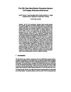
3 System Overview CSU Face Identification Evaluation System can be split into four basic phases: image data preprocessing, algorithm training, algorithm testing and analysis of results: see Figure1. Preprocessing reduces unwanted image variation by aligning the face imagery, equalizing the pixel values, and normalizing the contrast and brightness. Following preprocessing, there is a training phase. For the PCA, PCA+LDA and BIC algorithms, training creates subspaces into which test images are subsequently projected and matched. The training phase for the EBGM algorithm is different. There is no global subspace by the EBGM algorithm, and therefore no need to generate one from training imagery. However, the algorithm does require that specific landmark features be hand selected from a set of training, or model, images. All four algorithms have similar testing phases in that testing creates a distance matrix for the union of all images to be used either as probe images or gallery images in the analysis phase. The fourth phase and final phase performs analyses on the distance matrices. This includes computing recognition rates (csuAnalyzeRankCurve), conducting virtual experiments (csuAnalizePermute), or performing other statistical analysis on the data. See Section 8 for examples.
3.1 Imagery The CSU Face Identification Evaluation System was developed using frontal facial images from the FERET data set. Images normalized using the csuPreprocessNormalize utility are written out to an image file that contains pixel values in a binary floating point format (sun byte order). Older versions of our system used a suffix “.nrm” to designate these files. The current system generates “.sfi” files. These are very similar, the distinction is as follows:
6
������������������������������������������������������������������ ������������������������������������������������������������������������������������������������������������������������������� ������������������������������������������������������������������ ��Preprocessing ����������������������������������������������������������������������������������������������������������������������������� ������������������������������������������������������������������ ������������������������������������������������������������������������������������������������������������������������������� ������������������������������������������������������������������ ������������������������������������������Normalization ������������������������������������������������EBGM ������������Normalization ������������������������� ������������������������������������������������������������������ ������������������������������������������������������������������������������������������������������������������������������� Training Subspace Training
Baysian Training EBGM Localization
Testing EBGM Face Graph Subspace Project
Baysian Project EBGM Measure
Analysis
Rank Curve Testing
Permutation Testing
Standard Cumulative Match Curves
Probability Distribution for Recognition Rate
Figure 1: Overview of execution flow for the CSU Face Identification Evaluation System.
7
3.1.1
SFI Images
SFI stands for Single Float Image. This format is the standard for the CSU face recognition project. It was created at CSU as a floating point variant of pgm. It consist of multi channel raw floating point image data that is stored in Sun byte order. The images have a simple format similar to pgm with a short ASCII header (format_id, width, height, channels) followed by (32 bit) binary floating point values. 3.1.2
NRM Images
NRM is the designation adopted at CSU for images generated by the old NIST normalization code. This is a legacy format and is kept around for compatibility purposes. It is very similar to SFI only with out the header. This format is only supported by part of the CSU distribution. It is recommended that old codes are modified to use the SFI replacement.
3.2 Image Lists It is impossible to run experiments without first identifying sets of images to be used to train and test algorithms. Thus, we need files that store these image lists. In the original FERET evaluation, image list files were simple ASCII files with one image name per line. Some of our algorithms need to be able to know which images are of the same person, and this gave rise to a new file formatting convention. Specifically, each line contains one or more image of the same subject. Moreover, all images of a given subject must appear in one line. This convention will generalize to other data sets without hard coding subject naming conventions in the algorithms themselves. Therefore an image list should have the form: SubjectA_Image1.sfi SubjectB_Image1.sfi SubjectC_Image1.sfi SubjectD_Image1.sfi
SubjectA_Image2.sfi SubjectB_Image2.sfi SubjectC_Image2.sfi SubjectD_Image2.sfi
SubjectA_Image3.sfi SubjectB_Image3.sfi SubjectC_Image3.sfi SubjectD_Image3.sfi
The executable csuReplicates will produce a file of this form if given a list of FERET images. We refer to this as a subject replicates table, and the file is denoted using a file extension *.srt. Some of the tools are also capable of taking a flat list of image names (*.list), however it is recommended that only “.srt” lists be used. See usage statements for more information. This distribution includes many common image lists, including the training images, gallery images, and four standard probe sets used in the FERET evaluations. 3.2.1
Documentation on individual image lists included in Version 5.0
The following is a short description of the most important image lists that are provided as part of version 5.0. They are grouped loosely by functionality. FERET Data Preprocessing coords.3368: This file contains image names and eye coordinates for many frontal images in the FERET database. It includes five images that were added to the list later. There used to be more images with eye coordinates. Many of these images were computer generated alterations of other database images. For example, the images scaled to a different size, or the color of the shirts were inverted. For this reason the images are not acceptable for general experiments on face recognition algorithms. To reduce confusion the artificially generated images were eliminated. If an image is not within this set its validity should be questioned.
8
FERET Data Training The following files are used for the training phase of the algorithms. feret_training.srt: Standard file used for training PCA, LDA, and BIC. feret_training_x2.srt: This file contains a subset of the previous file that is limited to only two images per subject. ebgm70.srt: This file contains the names of seventy images and corresponding landmark location files that are used to create the bunch graphs for the EBGM algorithm. feret_training_cd.srt This is an alternative training file. This file contains images from the FERET database that were contained on the training CD originally distributed to labs that participated in the FERET evaluation. All these images are fair game for training for the FERET test. FERET Data Testing all.srt: This list contains all of the images with eye coordinates. During typical operation, each algorithm generates a distance matrix for every image in this set. Individual tests can run on the distance matrix to determine the performance on other tests such as fb, fc, dup1, dup2, or permute. all.hi.srt all.lo.srt: This is the all.srt file split into two parts. It is used on duel processor machines by processing half of the full image list at one time. FERET Data Experiments The following files are the four probe sets and the gallery (fa) used in the FERET Test. These files are used to create rank curves. • dup1.srt • dup2.srt • fafb.srt • fafc.srt • feret_gallery.srt Other files used for experiments are: list640.srt: This file is used for the permutation test. This list is of 160 subjects with four images each. This image list used with the csuAnalyzePermute tool described below was used in[1]. imagecovariates.cov: This contains many different statistics for the pixel values in the FERET images. facecovariates.cov: This file contains the covariate data about a subset of the FERET database, such as, gender, race, glasses, etc. facecovariates.srt: This is a file containing all of the images in the face covariates file.
9
Note that the two covariate files are not actually image lists, but instead compilations of covariate data associated with FERET images. So, for example, facecovariates.cov includes all the subject covariates used in our paper “A Statistical Assessment of Subject Factors in the PCA Recognition of Human Faces” [6] Other Miscellaneous Image Lists ebgm150.srt: This file is a list of all images that have manually selected landmark points for use with the EBGM algorithm. ebgm70.srt is a randomly selected subset of this list. list1024.srt: This file is a list of four images for each of 245 FERET subjects. It may be used as an alternate to list640.srt list1024_all_subset.srt list1024_subset.srt list2144.srt The following files are used with the CSU scrap shot database. The database is a small set of images taken from before 1925 CSU year books. These images are of low quality and should not be used for any experiments. • coords.scraps • scrap_all.srt • scrap_all_x4.srt • scrap_gallery.srt • scrap_probe.srt
3.3 Distance Files Each algorithm produces a distance matrix for all of the images in the testing list. This matrix is split up into distance files. One file is produced for every image in the list. Each line in these file contain the name of another image and the distance to that image. The file has the same name as the "probe image" and is placed in a distance directory. All algorithms assume that smaller distances are a closer match. In many cases the base metric will yield a similarity score, where higher similarity yields higher scores. When this is the case the similarity values are negated to produce a “distance like” metric. Some examples of this are the Correlation and MahCosine distance metrics in csuSubpace, and the Bayesian and Maximum Likelihood Metrics in the csuBayesian code.
3.4 Documentation With each release of the CSU Face Identification Evaluation System, the User’s Guide grows and we trust becomes more useful. It is hoped that all researchers intending to use our system first take the time to review this guide. In addition to information in the User’s Guide, it is helpful to be familiar with the types of experiments that we’ve conducted using the system, and the best documentation on these is through the papers available on our website [2]. For each of our tools, most current documentation and specific instructions as to options are available through the special command line argument “-help”. This command interface is updated with the code and will produce a descriptive usage statement that covers all of the arguments and options that the executables expect. So, for example, Figure shows the command line help for the csuSubspaceTrain executable.
10
Figure 2: Example of command line help for the csuSubspaceTrain executable.
4 Preprocessing Preprocessing is conducted using the executable csuPreprocessNormalize. The executable performs five steps in converting a PGM FERET image to a normalized image. The normalization schedule is: 1. Integer to float conversion - Converts 256 gray levels into floating point equivalents. 2. Geometric normalization – Lines up human chosen eye coordinates. 3. Masking – Crops the image using an elliptical mask and image borders such that only the face from forehead to chin and cheek to cheek is visible. 4. Histogram equalization – Equalizes the histogram of the unmasked part of the image. 5. Pixel normalization – scales the pixel values to have a mean of zero and a standard deviation of one. For an example image see Figure3 In order to preprocess imagery, the exact coordinates of the eyes must be provided. As mentioned above, the file containing eye coordinates for the FERET data is coords.3368 and it is kept in with the imagelists. Users wishing to use our system with their own data will need some either automated or manual way of geometrically normalizing images, and this may involve identifying eye coordinates by hand. Our csuPreprocessNormalize is a newly written piece of code that accomplishes many of the same tasks performed by code originally written at NIST called “facetonorm”. The NIST preprocessing code was used in the FERET evaluation and a slightly modified version was released in our earlier code releases. There were many problematic features of the NIST code, including a tendency to core dump for some combinations of arguments. Our new version is much more robust. It is not identical in function to the NIST code. For example, histogram 11
Figure 3: Example of a normalized FERET Image equalization in the new version is done only over the unmasked portions of the face. We recommend using this newer version.
5 CSU Subspace 5.1 Principle Components Analysis The first algorithm released by CSU was based on Principle Components Analysis (PCA)[8]. This system is based on a linear transformation in feature space. Feature vectors for the PCA algorithm are formed by concatenating the pixel values from the images. These raw feature vectors are very large (~20,000 values) and are highly correlated. PCA rotates feature vectors from this large, highly correlated subspace to a small subspace which has no sample covariance between features. PCA has two useful properties when used in face recognition. The first is that it can be used to reduce the dimensionality of the feature vectors. This dimensionality reduction can be performed in either a lossy or lossless manor. When applied in a lossy manor, basis vectors are truncated from the front or back of the transformation matrix. It is assumed that these vectors correspond to not useful information such as lighting variations (when dropped from the front) or noise (when dropped from the back). If none of the basis vectors are dropped it is a lossless transformation and it is possible to get perfect reconstruction for the training data based on the compressed feature vectors. The second useful property is that PCA eliminates all of the statistical covariance in the transformed feature vectors. This means that the covariance matrix for the transformed (training) feature vectors will always be diagonal. This property is exploited for some distance measures such as L1, MahAngle, and Bayesian based classifiers. Training PCA training is performed by the csuSubspaceTraining executable. The PCA is the default mode (it can also perform LDA training). The PCA basis is computed by the snapshot method using a Jacobi eigensolver from the Intel CV library. The basis vectors can be eliminated from the subspace using the cutOff and dropNVectors command line options. These methods are described in detail in[15]. The training program outputs a training file that contains a description of the training parameters, the mean of the training image, the eigenvalues or fisher values, and a basis for the subspace. Distance Metrics The csuSubspaceProject code is used to generate distance files. It requires a list of images and a subspace training file. The code projects the feature vectors onto the basis. It then computes the 12
distance between pairs of images in the list. The output is a set of distance files containing the distance from each image to all other images in the list. The distance metrics include city block (L1), Euclidean (L2), Correlation, Covariance, Mahalinobis Cosine (PCA only), and LDA Soft (LDA only).
5.2 Linear Discriminant Analysis The second algorithm is Linear Discriminant Analysis (PCA+LDA) based upon that written by Zhao and Chellapa[16]. The algorithm uses Fisher’s Linear Discriminants. LDA training attempts to produce a linear transformations that emphasize differences between classes while reducing differences within classes. The goal is to form a subspace that is linearly separable between classes. When used in the Face Identification and Evaluation System each human subject forms a class. LDA training requires training data that has multiple images per subject. LDA training is performed by first using PCA to reduces the dimensionality of the feature vectors. After this LDA is performed on the training data to further reduces the dimensionality in such a way that class distinguishing features are preserved. A final transformation matrix is produced by multiplying the PCA and LDA basis vectors to produce a full input image to LDA space transformation matrix. The final output of the LDA training is the same as PCA. The algorithm produces a set of LDA basis vectors. These basis vectors produce a transformation of the feature vectors. Like the PCA algorithm, distance metrics can be used on the LDA feature vectors. Training Like PCA, LDA training is performed by the csuSubspaceTraining executable. This algorithm is enabled using the -lda option. PCA is first performed on the training data to determine an optimal basis for the image space. The training images are projected onto the PCA subspace to reduce their dimensionality before LDA is performed. Computationally LDA follows the method outlined by [4]. A detailed description of the implementation can be found in[7] . Distance Metrics The csuSubspaceProject code is also used to generate distance files for LDA.
5.3 Common Distance Measures The following four common distances measures are available in csuSubspaceProject. 5.3.1
CityBlock (L1) DCityBlock (u, v) = ∑ |ui − vi | i
5.3.2
Euclidean (L2)
DEuclidean (u, v) =
13
r
∑(ui − vi )2 i
5.3.3
Correlation
This is a standard correlation measure between two vectors with one major caveat. Because all subsequent processing treats these measures as distance, the correlation mapped into the range 0 to 2 as follows: correlation 1 goes to 0 correlation -1 goes to 2. SCorrelation (u, v) =
5.3.4
∑i (ui − ¯u)(vi − ¯v) q q ¯2 ¯2 ∑i (vi −v) i −u) (N − 1) ∑i (u N−1 N−1
DCorrelation (u, v) = 1 − SCorrelation (u, v)
Covariance
This is the standard covariance definition, it is the cosine of the angle between the two vectors. When the vectors are identical, it is 1.0, when they are orthogonal, it is zero. Thus covariance and the associated distance are: ∑i ui vi q SCovariance (u, v) = q 2 ∑i ui ∑i v2i
DCovariance (u, v) = 1 − SCovariance (u, v)
5.4 Mahalinobis Based Distance Measures CSU Face Recognition System from its creation up through version 4.0 provided a distance metric labeled “Mahalinobis Angle” or “MahAngle” as its primary distance metric for the Principle Components Analysis (PCA) algorithm. This name was somewhat deceptive as the distance metric had very little to do with Mahalinobis space or angle measurement. For this reason we have decided to deprecate the old MahAngle distance metric in favor of a properly formulated angle based Mahalinobis metric. To make sure there is no confusion with the old distance metrics we have renamed MahAngle to YamborAngle. We have also added YamborDist which is based on a distance metric presented in Wendy Yambor’s thesis[15]. Both these metrics were improperly presented as Mahalinobis based metrics and were mistakenly adopted into the CSU Face Recognition System. We have added a proper version of an angle measure between images in Mahalinobis space. This measure is the cosine of the angle between two images after they have been scaled by the sample standard deviation along each dimension, and this new MahCosine takes the place of the old MahAngle for most experiments. For completeness MahL1 and MahL2 were also added but are not covered in this paper. Since these Mahalinobis measures and Mahalinobis like measures are a possible source of confusion, let us here give a short and concise explanation of the Mahalinobis distance metrics used in the CSU system, and explain there relationship to the old metrics. 5.4.1
Conversion to Mahalinobis Space
The first step in computing Mahalinobis based distance measures is to understand the transformation between image space and Mahalinobis space. PCA is used to find both the basis vectors for this space and the sample variance along each dimension. The output of PCA are eigenvectors that give rotation into a space with zero sample covariance between dimensions, and a set of eigenvalues that are the sample variance along each of those dimension. Mahalinobis space is “defined” as a space where the sample variance along each dimension is one. Therefore, the transformation of a vector from image space to feature space is performed by dividing each coefficient in the 14
vector by its corresponding standard deviation. This transformation then yields a dimensionless feature space with unit variance in each dimension. Because this paper will soon deal with the similarity between two vectors we will define two vectors u and v in the unscaled PCA space and corresponding vectors m and n in Mahalinobis space. First, we define λ i = σ2i where λi are the PCA eigenvalues, σ2i is the variance along those dimensions and σ i is the standard deviation. The relationship between the vectors are then defined as: mi =
5.4.2
ui σi
ni =
vi σi
Mahalinobis L1
This measure is exactly the same as the City block measure only the distances are scaled to Mahalinobis space. So for images u and v with corresponding projections m and n in Mahalinobis space, Mahalinobis L1 is: DMahL1 (u, v) = ∑ |mi − ni | i
5.4.3
Mahalinobis L2
This measure is exactly like Euclidean distance only computed in Mahalinobis space, so for images u and v with corresponding projections m and n in Mahalinobis space, Mahalinobis L2 is: DMahL2 (u, v) =
r
∑(mi − ni )2 i
This is what most people mean if they use the phrase Mahalinobis distance 5.4.4
Mahalinobis Cosine
Mahalinobis Cosine is the cosine of the angle between the images after they have been projected into the recognition space and have been further normalized by the variance estimates. So, for images u and v with corresponding projections m and n in Mahalinobis space, the Mahalinobis Cosine is: SMahCosine (u, v) = cos(θmn ) =
m·n |m| |n| cos(θmn ) = |m| |n| |m||n|
DMahCosine (u, v) = −SMahCosine (u, v)
This is essentially the covariance between the images in Mahalinobis space.
5.5 Deprecated Measure Mahalinobis Angle is now Yambor Angle. The Mahalinobis Cosine is new to the CSU Face Identification Evaluation System as of version 5.0. Previously, a measure based originally on work by Moon and subsequently refined by Yambor was provided. As previously mentioned, this measure was perhaps not very wisely called MahAngle and will from this point forward be called Yambor Angle. Yambor angle began with an earlier measure used by Moon that defined the distance between two image as follows: 15
k
Dm (u, v) = − ∑
i−1
s
λi ui vi λi − α 2
This measure was reported to be better than the standard measures when used in conjunction with a standard PCA classifier[10]. During Yambor’s work at CSU[14] she found a simpler variant performed better a “Mahalinobis distance” as: k 1 DYamborDistance (u, v) = − ∑ √ ui vi i−1 λi Most of the experiments performed by Yambor assumed a pre-processing step that normalized all image in PCA space to be of unit length. To generalize the measure intended by Yambor to images that may not be of unit length, the measure may be written as: DYamborAngle (u, v) = −
1 k 1 ∑ √λi ui vi |u| |v| i−1
There are are two reasons why Mahalinobis Angle was a poor choice of names for the Yambor Angle. First, as with the YamborDistance the measure looses the dimensionless properties of the Mahalinobis space. Second, the value is scaled by the lengths of the PCA space vectors instead of the Mahalinobis vectors. It is difficult to describe in precise terms exactly what the Moon measure or later the Yambor measures are computing. Unlike the Mahalinobis variants defined in the previous section, they have no simple interpretation relative to Mahalinobis space. However, these measure have performed well in the face recognition domain[1] and we an probably others who have used versions of the CSU Face Identification Evaluation System prior to version 5.0 have probably made use of the YamborAngle measure. Our recent experience suggests to us that Mahalinobis Cosine performs even better than any of these previous measures, and so it is now the standard default. Thus, while studies done in the past using the Yambor Angle (then called MahAngle) are valid, our recommendation is that users adopt Mahalinobis Cosine as the standard base-line for the PCA algorithm.
5.6 LDASoft, a PCA+LDA Specific Distance Measure The soft distance measure proposed by WenYi Zhao is essentially the L2 norm with each axis weighted by the associated generalized eigenvalue (λ) for the generalized eigenvalue problem used to find the Fisher basis vectors, raised to the the power 0.2. This is not obvious, but considerable discussion of this design appears in WenYi Zhao’s Dissertation[17]. DLDASo f t (u, v) = ∑ λi0.2 (ui − vi )2 i
6 Bayesian Intrapersonal/Extrapersonal Classifier (csuBayesian/BIC) The third algorithm in the CSU distribution is based on an algorithm developed by Moghaddam and Pentland[9]. There are two variants of this algorithm, a maximum a posteriori (MAP) and maximum likelihood (ML) classifier. This algorithm is interesting for several reasons, including the fact that it examines the difference image between two photos as a basis for determining whether the two photos are of the same subject. Difference images which originate from two photos of different subjects are said to be extrapersonal whereas images which originate from two photos of the same subject are said to be intrapersonal. 16
The key assumption in Moghaddam and Pentland’s work is that the particular difference images belonging to the intrapersonal and extrapersonal difference images originate from distinct and localized Gaussian distributions within the space of all possible difference images. The actual parameters for these distributions are not known, so the algorithm begins by extracting from the training data, using statistical methods, the parameters that define the Gaussian distributions corresponding to the intrapersonal and extrapersonal difference images. This training stage, called density estimation, is performed through Principle Components Analysis (PCA). This stage estimates the statistical properties of two subspaces: one for difference images that belong to the intrapersonal class and another for difference images that belong to the extrapersonal class. During the testing phase, the classifier takes each image of unknown class membership and uses the estimates of the the probability distributions as a means of identification. Training In version 5.0 of the distribution, the program “csuBayesianTrain” is used to train the Bayesian classifier. It is no longer necessary to run “csuMakeDiffs” or to run “csuSubspaceTrain” for each of the interpersonal and extrapersonal spaces as was required in version 4.0. The new program “csuBayesianTrain” combines these tasks into one. For each of the interpersonal and extrapersonal spaces, the PCA basis is computed by the snapshot method using a Jacobi eigensolver from the Intel CV library. The basis vectors can be eliminated from the subspace using the cutOff and dropNVectors command line options. These methods are described in detail in[15]. The training program outputs two training files, one for each subspace. The training files contains a description of the training parameters, the mean of the training image, the eigenvalues and a set of basis vectors for the subspace. Distance Metrics The “csuBayesianProject” code is used to generate distance files. It requires a list of images and two subspace training files that are written by “csuBayesianTrain” (one for the extrapersonal difference images and another for the intrapersonal difference images). The code projects the feature vectors onto each of the two sets of basis vectors and then computes the probability that each feature vector came from one or the other subspace. The output is a set of distance files containing the distance from each image to all other images. The similarities may be computed using the maximum a posteriori (MAP) or the maximum likelihood (ML) methods. From a practical standpoint, the ML method uses information derived only from the intrapersonal images, while the MAP method uses information derived from both distributions. A detailed technical report describing the BIC algorithm is nearing completion and should be posted to our website in May 2003. Anyone in need of a draft earlier may contact us directly.
7 Elastic Bunch Graph Matching (csuEBGM) The CSU EBGM is based on an algorithm from University of Southern California[11]. The algorithm locates landmarks on an image, such as the eyes, nose, and mouth. Gabor jets are extracted from each landmark and are used to form a face graph for each image. A face graph serves the same function as the projected vectors in the PCA or LDA algorithm; they represent the image in a low dimensional space. After a face graph has been created for each test image, the algorithm measures the similarity of the face graphs. The EBGM algorithm uses a special process to normalize its images. EBGM images can be produced by running the script ”EBGMPreprocessing.sh”. This script will call the normalization code with the special parameters needed to create EBGM images. The EBGM algorithm is divided into three executables that perform landmark localization, face graph creation, and similarity measurement. These programs should be run using the script “EBGM_Standard.sh”.
17
Landmark Localization: The purpose of the landmark localization process is to automatically locate landmark locations on novel images. Landmarks are found using the program csuEBGMGraphFit. The output of this program is a file for each novel image that contains the automatically located landmark locations for that image. This program has two high level parts: bunch graph creation and landmark location localization. Face Graph Creation: The program csuEBGMFaceGraph uses the automatically located landmark locations from the previous process and normalized imagery to create face graphs for every image in the database. Similarity Measurement: The program csuEBGMMeasure, of the EBGM algorithm is to produce a distance matrix for the FERET database. A detailed technical report based-upon David Bolme’s Masters Thesis is nearing completion and will be posted to our website in May 2003. Anyone in need of a draft earlier may contact us directly.
8 Analysis There are two basic analysis tools provided with version 5.0 of the CSU Face Identification Evaluation System. The first generates cumulative match curves of the type commonly reported in the FERET evaluation[12] and the later Vendor Test 2000[3]. This tool is called csuAnalyzeRankCurve. The other tool performs a permutation of probe and gallery images analysis to generate a sample probability density curve for recognition rates at different recognition ranks. This tool was used to perform the nonparametric analysis of PCA versus PCA+LDA reported in[1]. This tool is called csuAnalyzePermute. Both of these tools are described in more detail below.
8.1 CSU Rank Curve The rank curve tool csuAnalyzeRankCurve is used to generate the standard FERET cumulative match curves. It takes a probe and gallery imagelist. It ultimately generates an ASCII file that can be easily used to generate a plot of a cumulative match curve. It does this internally by first computing the rank of the closest gallery image of the same subject for each probe image. A rank curve is then generated by summing the number of correct matches for each rank. There are in practice two files produced by csuAnalyzeRankCurve, and both contain interesting information. It will be easiest to explain these files using an example, so let us consider the results of running our runAllTests_feret.sh script followed by the generateFeretResults.sh. Just a note, these two script will do a great deal and we will return to this case repeatedly in explaining the analysis code. Also, as mentioned above, you will need to obtain your own copy of the FERET image data[5] prior to trying this test and you should also be prepared to tie up a computer for several days: the Bayesian algorithm in particular takes a lot of time to run. Returning to the output from csuAnalyzeRankCurve, for each probe set two files will be generated, one with image rank data and the other with the cumulative match scores at different recognition ranks. So, for the specific case of probe set dup2, there are two files: DUP2_images.txt and DUP2_Curve.txt. Both files contain ASCII tabular data that is tab delimited. These file can be subsequently processed by other programs and also loaded directly into common spreadsheet programs. Table1 shows the first 10 rows of the DUP2_images.txt file. The first row contains the column headers. The first column contains the names of the probe images in the analysis, note the full file names including file type suffix are typically carried along. The remaining columns summarize recognition rank data for each distance measure being studied. In this case, the full distance names are: • distances/feret/Bayesian_MAP 18
• distances/feret/Bayesian_ML • distances/feret/EBGM_Standard • distances/feret/LDA_Euclidean • distances/feret/LDA_ldaSoft • distances/feret/PCA_Euclidean • distances/feret/PCA_MahCosine. These full names actually reference the specific directories in which the distances files are stored, and it is common to give these directories names that are understandable. For the sake of space in presentation, these names are shortened in Table1. The values in column 2, 3, etc. of Table1 are interpreted as follows. A zero means that for the corresponding probe image and distance measure, the first match of a gallery image of the same subject is found at position zero in the gallery sorted by increasing distance relative to the probe image. This is a somewhat long way of saying that zero means the best match is of the same subject. Likewise, a one means there is one gallery image of another subject that is closer than the gallery image of the same subject, and so on. This value is commonly called the recognition rank. Now, perhaps unfortunately, it has become common to speak of recognition at rank one when speaking of the best match, and this is a classic one-based versus zero-based counting issue. So, while the file carefully gives a zero, you will find us and others count a zero as a successful recognition at rank one. Once you are prepared for this adjustment in interpretation, it will hopefully not be too terribly off-putting. The recognition rank files, such as DUP2_images.txt, are worth studying in their own right. Observe for example the first probe image 00019ba010_960521.sfi. The difference between a PCA algorithm using Euclidean distance and one using Mahalinobis Cosine is the difference between a recognition rank of 59 versus 0. In other words, for this particular probe image, PCA does perfectly using Mahalinobis Cosine and relatively poorly using Euclidean distance. It is also worth noting that large recognition ranks do appear. For DUP2_images.txt, the gallery contains 1,196 images, and recognition ranks in the seven and eight hundreds are present in this table. The recognition rank file also provides some insight into how the cumulative match curves are generated. To compute the recognition count, i.e. how many images are correctly recognized by going a particular depth into the list of sorted gallery images, all that is needed is to scan down a column and count how often the recognition rank is less than or equal to the desired depth. So, to compute the recognition count for the BIC algorithm using the MAP distance measure at rank one, scan down the column counting how often a zero appears. For recognition count at rank two, count how often a value less than two appears, and so on. Recall Table 1 only shows the first 9 of the 234 probe images in probe set dup2, so in this example counting is performed over 234 rows in the table. Be aware the term recognition count is distinct from recognition rate. Recognition count is the actual number of probe image correctly recognized at a given rank, while recognition rate is the recognition count divided by the total number of probe images. This discussion of recognition counts leads us naturally into the second file produced by csuAnalyzeRankCurve, which for this example is DUP2_Curve.txt. Table 2 shows the first 10 rows of this file. The first row contains column headers and the header of the first column indicates this columns shows the recognition rank, starting at zero and running through the number of probes in the probe set. The remaining columns come in pairs, a recognition count and a recognition rate for a given distance measure at the indicated recognition rank. In Table 2, these column headers have been abbreviated in order that the table might format well here. What one can see quickly by scanning a given row is the different recognition rates for each algorithm at a given rank. So, for recognition rank one1 , the BIC algorithm using the ML distance measure has a recognition rate of 0.32: higher 1 With apologies, realize that this is a case of switching from zero-based to one-based counting, and the row with rank zero is what we are calling recognition rank one. Future releases of our system will try to standardize this nomeclature.
19
ProbeName 00019ba010_960521.sfi 00019bj010_960521.sfi 00029ba010_960521.sfi 00029bj010_960521.sfi 00029fa010_960530.sfi 00029fa010_960620.sfi 00029fa010_960627.sfi 00029fb010_960530.sfi 00029fb010_960620.sfi
Rank 0 1 2 3 4 5 6 7 8 9
BIC MAP 74 0.31 88 0.37 97 0.41 106 0.45 109 0.46 116 0.49 121 0.51 125 0.53 130 0.55 137 0.58
Table 1: First 10 rows of the DUP2_images.txt file. BIC MAP BIC ML EBGM LDA Euc. LDA ldaSoft 9 12 81 460 481 404 463 280 828 800 0 0 21 21 11 1 0 41 222 211 0 0 668 2 3 3 2 778 198 136 0 0 412 189 224 0 0 550 1 2 0 0 743 27 24
Table 2: First 10 rows of the DUP2_Curve.txt file. BIC ML EBGM LDA Euc LDA ldaSoft PCA Euc 75 0.32 52 0.22 32 0.13 32 0.13 33 0.14 89 0.38 70 0.29 43 0.18 41 0.17 43 0.18 100 0.42 89 0.38 53 0.22 52 0.22 48 0.20 109 0.46 95 0.40 57 0.24 55 0.23 56 0.23 114 0.48 101 0.43 62 0.26 59 0.25 63 0.26 118 0.50 109 0.46 63 0.26 62 0.26 68 0.29 123 0.52 110 0.47 64 0.27 64 0.27 69 0.29 128 0.54 115 0.49 65 0.27 67 0.28 74 0.31 130 0.55 118 0.50 66 0.28 68 0.29 77 0.32 132 0.56 119 0.50 68 0.29 69 0.29 79 0.33
PCA Euc. 59 423 8 35 77 105 38 99 114
PCA MahCos. 0 228 0 35 403 650 192 193 927
PCA MahCos 51 0.21 63 0.26 68 0.29 69 0.29 70 0.29 75 0.32 80 0.34 81 0.34 83 0.35 86 0.36
than any another other algorithm distance measure combination. Recall from the original FERET evaluation that probe set dup2 is a difficult test. The curve.txt files are easily used to generate standard cumulative match curves. The version 5.0 distribution comes with scripts to generate cumulative match curve data for the four standard FERET probe sets, specifically the runAllTests_feret.sh and generateFeretResults.sh scripts mentioned above. The curves themselves are produced by a small Python program that in turn uses GNUplot to generate the figures. This program is in extras/compareRankCurves.py. Examples of these figures appear in Figure 4 and 5 . The actual cumulative rank curves are similar to those shown in the original FERET evaluation[12]. However, they are not identical, nor would we expect them to be identical. There are many differences including new algorithm implementations, new image preprocessing code and perhaps most importantly different training image sets. Keeping those caveats in mind, our script will pre-process the FERET imagery, train the algorithms, run the algorithms to generate distance matrices, and finally build cumulative match curves for the standard set of FERET gallery images and each of the four standard FERET probe image sets. This script is a good baseline, or point of departure, for people wanting to understand what was done in the FERET evaluation and wanting to adapt it to their own purposes.
8.2 CSU Permute The CSU permutation of probe and gallery images tool, csuAnalyzePermute, performs virtual experiments using distance files. It does this by taking random permutations of the probe and gallery sets and then performs 20
1 0.95 0.9
Rate
0.85 0.8 0.75 PCA_Euclidean LDA_Euclidean EBGM_Standard Bayesian_ML LDA_ldaSoft PCA_MahCosine Bayesian_MAP
0.7 0.65 0.6 0
5
10
15
20
25 Rank
30
35
40
45
50
45
50
(a) 1 0.9 0.8 0.7
Rate
0.6 0.5 0.4 PCA_Euclidean LDA_Euclidean EBGM_Standard Bayesian_ML LDA_ldaSoft PCA_MahCosine Bayesian_MAP
0.3 0.2 0.1 0 0
5
10
15
20
25 Rank
30
35
40
(b) Figure 4: Cumulative Match Curves: a) FERET FA Probe Set. b) FERET FC Probe Set.
21
0.85 0.8 0.75 0.7
Rate
0.65 0.6 0.55 0.5
PCA_Euclidean LDA_Euclidean EBGM_Standard Bayesian_ML LDA_ldaSoft PCA_MahCosine Bayesian_MAP
0.45 0.4 0.35 0.3 0
5
10
15
20
25 Rank
30
35
40
45
50
45
50
(a) 0.8 0.7
Rate
0.6 0.5 0.4 PCA_Euclidean LDA_Euclidean EBGM_Standard Bayesian_ML LDA_ldaSoft PCA_MahCosine Bayesian_MAP
0.3 0.2 0.1 0
5
10
15
20
25 Rank
30
35
40
(b) Figure 5: Cumulative Match Curves: a) FERET Dup 1 Probe Set, b) FERET Dup 2 Probe Set.
22
nearest neighbor classification. It then generates a sample probability distribution for recognition rate under the assumption that probe and gallery images are interchangeable for subjects. To read more about the methodology lying behind csuAnalyzePermute and how it may be used to characterize the performance of an algorithm see our paper from CVPR 2001[1]. Also note that an alternative means of computing error bars has been developed by Ross Micheals and Terry Boult[13]. To run csuAnalyzePermute distances files for all of the images in the study must already be computed. Then, the program needs a list of subjects with at least three replicate images per subjects. Our typical FERET studies use imagelists with four replicates per subject, and two of these imagelists are list1024.srt and list640.srt. The program then proceeds to randomly assemble probe and gallery sets and compute recognition rates. It typically does this 10,000 times. Say the algorithm is running on a test set with four replicate images per subject, then it will select at random one of the four images for each subject to serve as a probe image and one of the remaining three to serve as the gallery image. The precise random selection is procedure is described in [1]. The tool csuAnalyzePermute as been enhanced in version 5.0 to also do comparison of multiple algorithm/distance combinations. Thus, as with csuAnalyzeRankCurve, it takes as an argument a list of distance matrices, or to be more precise, a list of directories containing distance files. The new version of csuAnalyzePermute will compute three files for each distance measure along with a summary file. As before, it is probably easiest to explain these files with an example generated by the combination of the runAllTests_feret.sh and generateFeretResults.sh scripts. So, for example, the files PermBayesian_ML_HistCounts.txt, PermBayesian_ML_HistProbs.txt and PermBayesian_ML_CMCurve.txt are generated for the distance file produced by the BIC (Bayesian) algorithm using the Maximum Likelihood (ML) distance. The resulting files are tab delimited tables in ASCII format, and Figure 6 shows portions of the files PermBayesian_ML_HistCounts.txt and PermBayesian_ML_HistProbs.txt loaded into Microsoft Excel. The top row in both tables in Figure 6 are the same and are column headers. Likewise, the first two columns are identical. The first column, rc, is an exact recognition count running from 0 to the number of probe images. The second column is the recognition rate: recognition count divided by the number of probe images. In the histogram count table, the third column labeled r1 indicates how many time out of 10,000 randomly generated probe and gallery sets the algorithm correctly recognized exactly rc subjects. So, looking at the upper left portion of the top table, we see that the BIC algorithm using the Maximum Likelihood distance exactly recognized 100 subjects 2 times in 10,000 trials. Scanning down the r1 column, the peak in this histogram is 992 at recognition count 116, indicating that 116 subjects were recognized correctly more often than any other single number of subjects. The second table, Figure 6b, is the same as Figure 6a with one exception, the histogram counts are divided through by the number of trials: 10,000. However, the interpretation is now very elegant, each column starting with r1 is a sample probability distribution for recognition count, or equivalently recognition rate. Column r1 corresponds to recognition rank 1, r2 to recognition rank 2, etc. It is a relatively simple matter to compute the average recognition rate at each rank, as well as the mode of the distribution at each rank. Perhaps more importantly, it is also possible to compute a two-sided confidence interval. This is done by simply identifying the central portion of each distribution accounting for 95 percent of the outcomes. To be even more precise, to find the lower bound on the confidence interval, our algorithm starts at rc equal to 0 and sums the values in the histogram until reaching 250. The cutoff 250 being 0.025 percent of 10,000. The analogous operation is performed coming down from the top to compute the upper bound. The third file produced by csuAnalyzePermute gives the average, mode and upper and lower confidence bounds on recognition count for rank 1, 2, etc. It is essentially a cumulative match curve with 95 percent confidence error bars. Table 3 shows the first 10 lines of the file PermBayesian_ML_CMCurve.txt. The first row contains column headers, and the columns are: the recognition rank, the lower bound on the 95 percent confidence interval, the mode of the probability distribution, the upper bound on the confidence interval and the mean recognition count. From these files, it is relatively simple to generate cumulative match curves with associated error bars. However, do note that this file records recognition counts, and all values must be divided by the number of probe images to arrive at recognition rates. 23
(a)
(b) Figure 6: Portions of the sample recognition rate distribution files generated by csuAnalyzePermute: a) the file PermBayesian_ML_HistCounts.txt containing the raw histogram counts of how often an algorithm recognized exactly k subjects at rank 1, 2, etc., b) the file PermBayesian_ML_HistProbs.txt containing the sample probability distribution derived from the histogram obtained by dividing through by the number of random trials: 10,000 in this case. 24
Table 3: The first ten lines of the file PermBayesian_ML_CMCurve.txt. This files provides a cumulative match curve with error bars. rank 1 2 3 4 5 6 7 8 9
lower 107 116 121 124 126 128 130 132 133
mode 116 123 128 132 134 136 137 138 139
upper 124 132 136 138 140 142 144 145 146
mean 115.5 123.9 128.2 131.1 133.4 135.3 137.0 138.5 139.8
Figure 7 shows these curves for the BIC algorithm using the Maximum Likelihood distance compared to the standard EBGM algorithm. Recall that this comparison is over a set of 640 FERET images of 160 subjects where the random permutations of probe and gallery images were selected 10,000 times. The error bars overlap considerably over the entire range of the curve, and certainly at rank 1. Were this the only information available to us, it would be likely we would be forced to conclude that the difference between the two algorithms is not significant. However, as we discuss in more detail in [1], observing whether error bars overlap is a very weak and not terribly appropriate test. Better is to compute the actual difference in recognition rates for each of the 10,000 trials, and then look at the distribution of this new random variable. Interpreting the resulting distribution is relatively easy, since a predominance of positive values indicates one algorithm is better, a predominance of negative values indicates the other algorithm is better, and a distributions centered around zero indicated there is no difference between the algorithms. csuAnalyzePermute carries out this test for all pairs of algorithm/distances-matrices it is given. The results are tabulated and placed in a web-page. An example of this webpage for the scripts runAllTests_feret.sh script followed by the generateFeretResults.sh is shown in Figure 8. The page first lists the algorithms compared, followed by statistics summarizing the sample distributions for each of the algorithms. In this case, the permutation results are shown for seven algorithm and distance measure combinations. The last table at the bottom provides the pairwise comparisons based upon the difference in recognition rate statistic. In all cases, the algorithm found to do better is shown in red. However, the probabilites are only highlighted when they are above a standard 95 percent confidence threshold. So, in the second to last row visible in the table we see that the pairwise test between the Bayesian algorithm using the maximum likelihood distance is significantly better than the EBGM algorithm. Thus we see that the paired test is more discriminating then is simply checking for overlap in error bars. The primary reason for the difference is that some apparently some probe and gallery choices are harder for both algorithms, and others are easier for both algorithms, so while the overall variation in recognition rates of the 10,000 trials is moderately large, the variation between the algorithm is somewhat smaller and more importantly the two algorithms are moving together.
9 Conclusion The CSU Face Identification Evaluation System has grown into a moderately large and complex system despite our on-going efforts to keep it simple and to the best of our abilities “vanilla”. If you have already taken the time to read the User’s Guide, you hopefully have had many of your questions answered with regards to what the system 25
Figure 7: This figure compares our PCA and Bayesian algorithms. The rank curves include 95% error bars that were estimated by csuPermute. The error bars show that there is no significant difference between PCA and Maximum Likelihood when trained on the FERET training set. can and cannot accomplish. As should be clear, it is certainly is not intended to give real-time demonstrations of face recognition. However, it is to our knowledge the most complete package of open source face recognition algorithms and includes the most complete set of associated analysis tools. The work at CSU studying and refining the four algorithms continues, and for the BIC and EBGM algorithms in particular, there is still more that needs to understood about algorithm configuration. That performance levels on the four standard FERET probe sets for these algorithms is not comparable to that achieved by the algorithms original creators in the FERET tests, and this strongly suggests that tuning plays a very significant role in how these algorithms perform in practice. The team at CSU is interested in feedback from users. Over the period from November 1, 2002 to April 30, 2003, Version 4.0 of the system was downloaded 1,867 times. Many researchers are giving the system a try and we’re already aware of several major studies that have been conducted using it. We would very much like to hear back from users regarding the outcomes of their own studies, and we are of course open to suggestions for future releases.
10 Acknowledgments This work supported by the Defense Advanced Research Projects Agency under contract DABT63-00-1-0007
26
Figure 8: Web summary generated by csuAnalyzePermute
27
References [1] J. Ross Beveridge, Kai She, Bruce Draper, and Geof H. Givens. A nonparametric statistical comparison of principal component and linear discriminant subspaces for face recognition. In Proceedings of the IEEE Conference on Computer Vision and Pattern Recognition, pages 535 – 542, December 2001. [2] Ross Beveridge. Evaluation http:\\cs.colostate.edu\evalfacerec.
of
face
recognition
algorithms
web
site.
[3] Duane M. Blackburn, Mike Bone and P. Jonathon Phillips. Facial Recognition Vendor Test 2000. http://www.dodcounterdrug.com/facialrecognition/frvt2000/ frvt2000.htm, DOD, DARPA and NIJ, 2000. [4] Richard O. Duda, Peter E. Hart, and David G. Stork. Pattern Classification. John Wiley & Sons, second edition edition, 2001. [5] FERET Database. http://www.itl.nist.gov/iad/humanid/feret/. NIST, 2001. [6] Bruce A. Draper Geof Givens, J. Ross Beveridge and David Bolme. A statistical assessment of subject factors in the pca recognition of human faces. Technical report, Computer Science, Colorado State University, 2003. [7] J. Ross Beveridge. The Geometry of LDA and PCA Classifiers Illustrated with 3D Examples. Technical Report CS-01-101, Computer Science, Colorado State University, 2001. [8] M. A. Turk and A. P. Pentland. Face Recognition Using Eigenfaces. In Proc. of IEEE Conference on Computer Vision and Pattern Recognition, pages 586 – 591, June 1991. [9] B. Moghaddam, C. Nastar, and A. Pentland. A bayesian similarity measure for direct image matching. ICPR, B:350–358, 1996. [10] H. Moon and J. Phillips. Analysis of pca-based face recognition algorithms. In K. Boyer and J. Phillips, editors, Empirical Evaluation Techniques in Computer Vision. IEEE Computer Society Press, 1998. [11] Kazunori Okada, Johannes Steffens, Thomas Maurer, Hai Hong, Egor Elagin, Hartmut Neven, and Christoph von der Malsburg. The Bochum/USC Face Recognition System And How it Fared in the FERET Phase III test. In H. Wechsler, P. J. Phillips, V. Bruce, F. Fogeman Soulié, and T. S. Huang, editors, Face Recognition: From Theory to Applications, pages 186–205. Springer-Verlag, 1998. [12] P.J. Phillips, H.J. Moon, S.A. Rizvi, and P.J. Rauss. The FERET Evaluation Methodology for FaceRecognition Algorithms. T-PAMI, 22(10):1090–1104, October 2000. [13] Ross J. Micheals and Terry Boult. Efficient evaluation of classification and recognition systems. In IEEE Computer Vision and Pattern Recognition 2001, pages I:50–57, December 2001. [14] Bruce A. Draper Wendy S. Yambor and J. Ross Beveridge. Analyzing pca-based face recognition algorithms: Eigenvector selection and distance measures. In Second Workshop on Empirical Evaluation in Computer Vision, Dublin, Ireland, July 2000. [15] Wendy S. Yambor. Analysis of pca-based and fisher discriminant-based image recognition algorithms. Master’s thesis, Colorado State University, 2000. [16] W. Zhao, R. Chellappa, and A. Krishnaswamy. Discriminant analysis of principal components for face recognition. In In Wechsler, Philips, Bruce, Fogelman-Soulie, and Huang, editors, Face Recognition: From Theory to Applications, pages 73–85, 1998. 28
[17] W. Zhao, R. Chellappa, and P.J. Phillips. Subspace linear discriminant analysis for face recognition. In UMD, 1999.
29