The Detection of Fault-Prone Program Using a Neural Network Shuji Takabayashi1, Akito Monden1, Shin-ichi Sato2, Ken-ichi Matsumoto1, Katsuro Inoue1,3 and Koji Torii1 1 Graduate School of Information Science, Nara Institute of Science and Technology 8916-5 Takayama, Ikoma, Nara 630-0101, Japan 2 NTT DATA Corporation, Laboratory for Information Technology, Department of Research & Development Headquarters Kayabacho-Tower, 21-2, Shinkawa 1-chome, Chuo-ku, Tokyo 104-0033, Japan 3 Graduate School of Engineering Science, Osaka University 1-3 Machikaneyama-cho, Toyonaka, Osaka 560-8531, Japan {shuji-t, akito-m}@is.aist-nara.ac.jp,
[email protected], {matumoto, k-inoue, torii}@is.aist-nara.ac.jp ABSTRACT
many complex and fault-prone program modules, that will
This paper proposes a discriminant analysis method
increase the maintenance cost [6]. In order to lessen such
that uses a neural network model to predict the fault-prone
maintenance cost, we need to predict the fault-prone
program modules that will cause failure after the release. In
modules in advance, and to test them thoroughly or
our method, neural networks of a layered type are used to
sometimes even restructure them as new modules.
represent nonlinear relation among predictor variables and
To detect the fault-prone modules, we need to
objective variables. Since the relation among predictor
construct a discriminant model, that has multiple predictor
variables and objective variables is complicated in real
variables such as complexity measures of software, to
software, linear representation used in conventional
predict which module is faulty. Conventional linear
discriminant analysis is not suitable for the prediction
discriminant model is as follows [3]:
model. To evaluate the method, we have measured 20 metrics, as predictor variables, from a large scale software that have been maintained more than 20 years, and also measured the number of faults found after the release as objective variables. Result of the evaluation showed that prediction accuracy of our model is better than that of conventional linear model. KEYWORDS
discriminant analysis, AIC, neural network INTRODUCTION
Many companies have legacy software that had been developed many years ago and have been continuously modified and expanded till today. However, continuous modification and expansion in large scale software produce
P > 0 : classified as " modules which don' t include any faults" P = ∑ aj Nj + C P < 0 : classified as " module which j∈D include at least one fault " Where D denotes a set of subscript of predictor variables that are chosen out from variables that we measure, N i ( i = 1 ,…,n ) denotes an observation value, a i (i =1 , …, n) denotes a distinction coefficient, and C denotes a constant. However, this linear model is not suitable for the prediction model. In this model, there is an assumption that the effect of each factor to the software reliability is additive, i.e., independent of the other factors. It is, however, not plausible because the factors are mutually and complicatedly related to each other in real software. We
need a nonlinear analysis method using a nonlinear
Method for linear discriminant models
In order to construct a liner discriminant model, we
representation model. In this paper, we propose a nonlinear discriminant
take advantage of the relation between discriminant
analysis method that uses a neural network model to predict
statistical analysis and multivariate regression analysis. In
the fault-prone modules in large scale software. In the
multiple regression analysis, which is a multivariate
method, neural networks of a layered type are used to
analysis method [3], the relation among predictor variables
represent nonlinear relation among predictor variables and
and objective variables is represented by a linear equation,
objective variables. A layered neural network is a data
such as:
processing model that represents nonlinear relation among
Y = a0 + a1N1 + … + aiNi + E
the inputs and the outputs by simple processing units and weighted links connecting the units. To construct a prediction model, we need to know the
Where Y denotes the objective variable, Ni (i = 1, …, n)
most appropriate combination of predictor variables. This
denotes a predictor variable, ai (i = 0, …, n) denotes a
paper presents a method for selecting a combination of
coefficient, and E denotes the residual between the
predictor variables that strongly affect the existence of
predicted value and the actual value.
faults in programs. To select predictor variables, we use a
In order to discriminate the program modules into two
forward selection method [3], in which variables are added
groups, regression analysis can be used, as shown in figure
to a prediction model one by one. To evaluate prediction
1. In figure 1, the first group contains program modules that
models that have different numbers of predictor variables, a
have a fault, and the second group contains modules that
statistical information criterion AIC (Akaike’s Information
have no fault. N1, N2, Y1 and Y2 are defined as follows:
Criterion) was used [1]. Takada et al.[7] also proposed a software reliability
N1 = the number of modules belong to the first group.
prediction model that uses a neural network. However, their
N2 = the number of modules belong to the 2nd group.
model evaluates the reliability of a software development
Y1 = N2 / (N1 + N2)
project itself and predicts the number of faults during the
Y2 = N1 / (N1 + N2)
development, while our model evaluates the reliability of
First group
each program module and discriminates the fault-prone
Y1
modules after the release. In what follows, we first propose a nonlinear model Then describes the data used for the experiment, and explains how models were constructed in the experiment. Next, we discuss on the accuracy of linear and nonlinear models and lessons learned on the experiment. Finally the paper describes the conclusion.
Discriminant value Discriminant value Y
construction method, comparing it with a linear model.
Regression line 0
Y2 Second group
MODEL CONSTRUCTION METHOD
The proposed nonlinear model construction method is an extension of a linear model construction method. In this section, first we describe the linear method and then describe the nonlinear method.
Values of predictor variables N i Figure 1. Relation between discriminant analysis and regression analysis
In the model construction phase, in case a module
biased. It tends to become larger that the real logarithmic
belongs to the first group, the value of the objective variable
likelihood when the number of parameters is large. The
Y is set to Y1; and, in case a module belongs to the second
second term has the role of compensating the bias.
group, Y is set to -Y2. Since N1 and N2 are not equal, we
Therefore, we can use AIC to evaluate models that have
assign a weighted value.
difference numbers of parameters.
In the discriminant phase, the discriminant value Y obtained by this regression analysis is interpreted as
Method for nonlinear discriminant models
We use a neural network model of three layers
follows:
( Input layer, Intermediate Layer, and Output layer ) as a Y > 0: classified as first group.
nonlinear discriminant model. We fixed the number of
Y < 0: classified as second group.
intermediate layer units to 3. Predictor variables Ni are input to units on input layer; and, the objective variable Y is
Let us assume that objective variables and related
output from the unit on output layer. Each unit of input
variables are given. The method of selecting an appropriate
layer receives the value of a predictor variable and sends the
combination of predictor variables and constructing a
weighted value to the intermediate layer. In the intermediate
prediction model as follows:
layer and the output layer, each unit receives the weighted values from the beyond layer and sum them up. The unit
Step1. Construct 1-input prediction models. Models as
then nonlinearly transform the sum by a sigmoid function
many as the variables are constructed. Use a least
(g( σ )=2/(1+exp(- σ ))-1). A neural network, which is
square method to estimate model parameters.
composed of multiple processing units, is able to represent
Step2. Select the best models among the constructed models based on AIC, a statistical criterion. Step3. Construct new models by adding one more predictor
complicated relation among predictor variables and an objective variable. The
major
difference
from
the
linear
model
variable to the temporary best model. Models as many
construction model is that model parameters are estimated
as the remaining variables are constructed. Then return
by a learning algorithm.
to Step2. Step1. Construct neural network. Then, let them learn the Step 2 and 3 are repeated until no variable remains or the
relation between the objective and predictor variables.
goodness of the temporary best model becomes worse than
Models as many as the variables are constructed.
that of the less variable model. Finally the best model
Step2. Select the best models among the constructed models
among all of the constructed models is selected.
based on AIC.
As the statistical criterion of goodness of models, we
Step3. Construct new models by adding one more predictor
use AIC. AIC means the minus double of the logarithmic
variable to the temporary best model selected in Step2,
likelihood of a model against given data:
and let it learn the relation again. Models as many as the remaining variables are constructed. Then return to
AIC = (Number of samples) log (Residual sum of squares)
Step2.
+ 2(Number of parameters) To determine the link weights appropriately from In the above, the first term is the minus double of an
samples of predictor and objective variables, we use a
estimate of the logarithmic likelihood, and the second term
standard learning algorithm called error backpropagation
is the expected difference between the real logarithmic
algorithm [5].
likelihood and the estimate. The estimate of the first term is
DATA FOR THE EXPERIMENT
The Data we used for the experiment are collected
P2: The sum of nest level of each statement. P3: The numbers of loop nodes.
from large scale program developed by Japanese software
P4: The number of substitution variables.
company. This program has been maintained for about 20
P5: The number of reference variables.
years and modified and expanded many times during that
P6: The number of external substitution variables.
period. The program was written in an old programming
P7: The number of external reference variables.
language (called HPL) that is peculiar to the hardware. The
P8: The sum of level of each substitution variable.
number of faults and 20 kind of metrics are measured in
P9: The sum of level of each reference variables.
each file (module). In this case, the number of faults means the number of modifications done for correcting defects.
Group O (Other metrics)
The numbers of program modules we measured is 1436.
E1: Version number.
We classified the collected metrics into three groups
E2: Lapsed days from the first release.
from the difficulty of measuring. Since some metrics are not easy to measure, software developers cannot always collect all the metrics. Here, we classify metrics into 3 groups as follows:
EXPERIMENT
We have conducted an experiment to evaluate the performance of our nonlinear model, comparing it with a
・ Group T: Set of metrics that can be measured by lexical analysis (easy to measure).
linear model.
・ Group P: Set of metrics that can be measured by syntactical analysis (more difficult to measure).
groups at random. Each group has 718 modules. The first
・ Group O: Set of metrics that cannot be measured from source code.
second group is used for evaluating the constructed models.
At first, we divided 1436 program modules into two group is used for estimating the model parameters; and, the Then, we divided each group into two more groups: fault-free group and fault-prone group. Fault-free group
Actual metrics in each group are described below:
contains modules in which no fault was found after the release. Fault-prone group contains modules in which more
Group T (Metrics obtained by Token analyzer)
than one fault was found after the release. The rate of the
T1: Lines of code.
program in which the bug was actually contained is about
T2: The number of comment lines.
ten percent of the whole.
T3: The number of procedure-call statements and jump statements. T4: The number of the modules called from the target module. T5-T9: Halstead’s Software Science [6].
In the experiment, we constructed two types of models, one is a model using the linear discriminant analysis, and the other is a model using neural network. Furthermore, following three types of model were constructed in each model. Therefore, we have six types of model in total.
T5: Vocabulary. T6: Length.
・ Model A: Uses predictor variables of group T.
T7: Volume.
・ Model B: Uses predictor variables of group T and P.
T8: Difficulty.
・ Model C: Uses predictor variables of group T, P, and O.
T9: Effort. Table 1 and 2 show the variables selected by a forward Group P (Metrics obtained by Parser)
selection method, and the value of AIC measured for each
P1: Cyclomatic number [6].
model. Variables are added to the model as long as the value
of AIC decreases. For example, in Linear Model A, a metric Table 1. Processes of selecting predictor variables for linear models
from eight metrics of group T. Table 2. Processes of selecting predictor variables for non linear models
(a) Linear Model A Predictor Variables T5 T5, T8 T5, T8, T1 T5, T8, T1, T4 T5, T8, T1, T4, T3 T5, T8, T1, T4, T3, T2 T5, T8, T1, T4, T3, T2, T7
AIC 2523.99 2510.19 2494.24 2488.70 2483.26 2482.82 2483.42
(a) Nonlinear Model A Predictor Variables T5 T5,T1 T5,T1,T9 T5,T1,T9,T4 T5,T1,T9,T4,T8 T5,T1,T9,T4,T8,T7
(b) Linear Model B Predictor Variables T5 T5,P6 T5,P6,T8 T5,P6,T8,P4 T5,P6,T8,P4,T2 T5,P6,T8,P4,T2,P1 T5,P6,T8,P4,T2,P1,T4 T5,P6,T8,P4,T2,P1,T4,P9, T5,P6,T8,P4,T2,P1,T4,P9,P2 T5,P6,T8,P4,T2,P1,T4,P9,P2,T3 T5,P6,T8,P4,T2,P1,T4,P9,P2,T3,P8 T5,P6,T8,P4,T2,P1,T4,P9,P2,T3,P8,P7 T5,P6,T8,P4,T2,P1,T4,P9,P2,T3,P8,P7,P5 T5,P6,T8,P4,T2,P1,T4,P9,P2,T3,P8,P7,P5,T1
(b) Nonlinear Model B AIC 2523.99 2471.44 2458.96 2454.50 2438.02 2434.42 2431.06 2428.80 2425.75 2424.81 2423.88 2423.54 2418.86 2420.19
(c) Linear Model C Predictor Variables E1 E1,P6 E1,P6,T5 E1,P6,T5,P4 E1,P6,T5,P4,P8 E1,P6,T5,P4,P8,P1 E1,P6,T5,P4,P8,P1,P9 E1,P6,T5,P4,P8,P1,P9,T9 E1,P6,T5,P4,P8,P1,P9,T9,T7 E1,P6,T5,P4,P8,P1,P9,T9,T7,E2 E1,P6,T5,P4,P8,P1,P9,T9,T7,E2,T6 E1,P6,T5,P4,P8,P1,P9,T9,T7,E2,T6,T8 E1,P6,T5,P4,P8,P1,P9,T9,T7,E2,T6,T8,T4 E1,P6,T5,P4,P8,P1,P9,T9,T7,E2,T6,T8,T4,P2, E1,P6,T5,P4,P8,P1,P9,T9,T7,E2,T6,T8,T4,P2,T2 E1,P6,T5,P4,P8,P1,P9,T9,T7,E2,T6,T8,T4,P2,T2,T3 E1,P6,T5,P4,P8,P1,P9,T9,T7,E2,T6,T8,T4,P2,T2,T3,P7
AIC 2526.04 2514.52 2508.58 2503.50 2503.01 2506.94
AIC 2477.08 2447.76 2440.52 2422.48 2418.54 2415.38 2410.54 2407.08 2403.02 2400.26 2399.33 2398.28 2397.87 2396.60 2396.05 2395.73 2395.96
Predictor Variables T5 T5,P6 T5,P6,P9 T5,P6,P9,T1 T5,P6,P9,T1,T9 T5,P6,P9,T1,T9,T4 T5,P6,P9,T1,T9,T4,P3 T5,P6,P9,T1,T9,T4,P3,T8
AIC 2526.04 2453.06 2445.45 2437.33 2431.07 2428.97 2423.55 2429.33
(c) Nonlinear Model C Predictor Variables T5 T5,P6 T5,P6,E1 T5,P6,E1,P9 T5,P6,E1,P9,T1 T5,P6,E1,P9,T1,T8 T5,P6,E1,P9,T1,T8,E2
AIC 2526.04 2453.06 2442.20 2432.08 2419.00 2410.23 2413.04
We use three types of criterion (type I error, type II error, and accuracy) to evaluate the goodness of prediction models. Type I error is a percentage of cases where the model concludes that a module is fault-prone though it is not so in fact. Type II error is a percentage of cases where the model says that a module is fault-free though it is not so. Accuracy is a percentage of cases where the model distinguishes modules correctly. The results are showed in Table 3. Table 3(a) shows
T5 (Halstead’s Software Science Vocabulary) is selected at
the residual variance (prediction error) when we apply the
first. The value of AIC is 2523.99. Next, a metric T8
model to evaluation data. Table 3(b) shows type I error, type
(Halstead’s Software Science Difficulty) is selected. The
II error and accuracy.
value of AIC is 2510.19. This means two-variable model (using T5 and T8) is statistically better than one-variable
DISCUSSION
model (using T5). As we increase the number of variables,
As shown in the Table 3(a), we see that prediction
value of AIC decreases. And in six-variable model, the
error of nonlinear model has been improved as compared
value of AIC becomes the minimum. That is, six variables
with the linear model. In the linear model, residual of
(metrics) are selected as a predictor variable of a model
Model C is the smallest. In the nonlinear model, the residual
of Model B and Model C is almost the same and they are
constructing nonlinear models that discriminate fault-prone programs. Through an experiment of real software developments, we have shown that the proposed model
Table 3. Experimental Result
shows
(a)Residual
Linear Nonlinear
Model A
Model B
Model C
0.05477 0.05645
0.05715 0.04979
0.05486 0.04982
Nonlinear
Model A Model B Model C Model A Model B Model C
TypeI error
TypeII error
Accuracy
in
discrimination
than
conventional discriminant analysis. There are some other related researches reported.
74% 73% 75% 62% 70% 68%
1.2% 1.2% 1.1% 2.3% 1.3% 1.9%
79% 75% 77% 88% 82% 84%
they employ a principal–components procedure to reduce predictor variables. In the future, we are going to compare
better than that of Model A. Let us compare the accuracy between linear model and nonlinear model
performance
Munson et al.[4] also proposed a nonlinear model in which
(b) Error and Accuracy
Linear
better
(see Table 3(b)). Obviously, nonlinear
models show good results. In the nonlinear model, the accuracy of model A shows the best. Therefore, if we use the nonlinear model, we can obtain enough accuracy by collecting only few metrics, which can be measured by lexical analysis. So the effort of software developers will be lessened by use of the nonlinear model. As shown in table 3, type I error is improved at nonlinear model. On the other hand, type II error is not improved. However, this does not result in that linear model is a good model. There are tradeoffs between type I error and type II error. Linear models tend to discriminate many programs as fault-prone programs, and this causes the improvement of type II error while it causes the corruption of type I error. In this experiment, type I errors are not so good on the whole. This is because the data we used for the experiment had a unique character. We have counted the number of fault found in the programs after the release. Therefore, not so many faults were found. The rate of programs in which fault was found is less than 10 %. Hence, when we found only one fault, we considered as fault-prone program. So we couldn't enhance the difference of characteristics between the sound programs and dangerous programs. CONCLUSION
We have presented a method for systematically
the goodness between their model and our model. REFERENCES
[1] H. Akaike “A new look at the statistical model identification,” IEEE Trans. on Automatic Control, Vol. 19, No. 6, pp. 716-723, 1974. [2] K. Funahashi, “On the approximate realization of continuous mappings by neural networks,” Neural Networks, Vol. 2, No. 3, 1989. [3] H. Kume and E. Iizuka, “Regression analysis,” Iwatami, Tokyo, 1987. [4] J. C. Munson and T. M. Khoshgoftaar, “The detection of fault-prone programs,” IEEE Trans. on Software Engineering, Vol. 18, No. 5, pp. 423-433, May. 1992. [5] D. E. Rumelhart, G. E. Hinton and R.J. Williams, “Learning representations by backpropagating errors,” Nature, Vol. 323, pp. 533-536, 1986. [6] I. Sommerville, “Software engineering fourth edition,” Addison-Wesley, pp. 533-550, 1992. [7] Y. Takada, “A software prediction model using a neural network,” System and Computer in Japan, Vol.25, No. 14, 1994.