plexiglas disk is projected on a screen in front of a driver. .... 5 114" Disk Drive Color Monitor ..... very difficult to recover and usually there is no way to resume.
The Development and Use of the UMTRl Driving Simulator Paul Green Alan Olson
UMTRI
The University of Michigan Transportation Research Institute
Tubmicol 1.
R-ct
2.
No.
G n o m m t Accession
No.
3.
Rlpor, D#wmtatim Pogo
Recipimt's Catalog No.
UMTRI-89-25 4.
Titlo
ad
5. Report Date
Subtitle
-October, 1989
THE DEVELOPMENT AND USE OF THE UMTRI DRIVING SIMULATOR
6. Puforaing Orgonizotim C o l
8.
Parbrming Orgomirotion R.port NO.
7. hW1)
Paul Green and A l a n 01 son 9.
UMTRI -89-25 10.
P n b d n g O r ~ r r i z m t i mN.no m d U h e s s
U n i v e r s i t y o f Michigan T r a n s p o r t a t i o n Research I n s t i t u t e 2901 B a x t e r Road . Ann Arbor, M I 48109-2150 U.S.A. 12. *swing
IS.
Suppl-tsy
Agmncy NH
WorL Unit No. (TRAIS)
I I.Controct or Gfont NO. port and Period
13.
T P I.
14.
Sponsoring Agency Code
of
Covered
md Address
Notes
1'6. Abstract
T h i s paper d e s c r i b e s t h e development, o p e r a t i o n , and use o f t h e UMTRI d r i v i n g s i m u l a t o r . T h i s l o w - c o s t system c o n s i s t s o f a Commodore 64 computer, a p r o j e c t i o n v i d e o d i s p l a y , and a f u l l - s i z e v e h i c l e mockup. The s i m u l a t o r shows a s i n g l e - l a n e r o a d a t n i g h t and a l l o w s f o r r e c o r d i n g o f s t e e r i n g e r r o r a t r a t e s of up t o 10 Hz. A t l o w e r sampling r a t e s p e r f o r mance can be recorded f o r up t o two hours. The s i m u l a t o r has been used i n a v a r i e t y o f human f a c t o r s experiments t o occupy p e o p l e ' s a t t e n t i o n w h i l e t h e y c o n c u r r e n t l y do o t h e r d r i v i n g - r e 1 a t e d t a s k s such as r e a d i n g highway s i g n s , r e a d i n g i n s t r u m e n t panel d i s p l a y s , and responding t o brake lamps o f l e a d i n g v e h i c l e s . Those a p p l i c a t i o n s a r e d e s c r i b e d i n d e t a i l . Based on t h a t bxperience, t h e q u a l i t i e s d e s i r e d i n a d r i v i n g s i m u l a t o r a r e i d e n t i f i e d . I t i s c l e a r t h a t ease o f use, low o p e r a t i o n a l c o s t , and s u p p o r t i n g i n t e r c h a n g e a b l e i n p u t and o u t p u t d e v i c e s were more i m p o r t a n t t h a n p r o v i d i n g a h i g h f i d e l i t y s i m u l a t i o n o f t h e road scene o r v e h i c l e dynamics.
17.
Key Wordn
18.
!
D i s k i b t i m Stdamant
human f a c t o r s , ergonomics, human engineering, d r i v i n g simulation, simul a t o r s 19.
Security Classif. (of *is
Unclassified
1D.
k c u r i t y Classif. (of M s pmgo)
Uncl a s s i f ied
21.
No. of Poges
22. P r ~ c e
34 1
ACKNOWLEDGMENTS The development of the simulator was supported by a contract from the Amway Corporation. The mockup initially used was donated by the Ford Motor Company. The current mockup was donated by the Chrysler Corporation, with funds from several of their recent projects being used to make minor improvements to the software. Paul Green has managed its development and modified the user interface several times and, in addition, has written several support programs. Many other University of Michigan staff and students played key roles in the development of the UMTRI simulator. Sue Adams developed a preliminary version in BASIC. Alan Olson--a master of assembly language--wrote the display driver, the heart of the program, the initial user interface, in fact, most of the code in the current version of the program. Mike Scheller tested the software and revised the interface and, Kim Clack was responsible for the latest set of interface modifications. Mike Campbell was responsible for all of the electrical work and worked magic by getting the projection video system to focus. More recently, John Boreczky has done his share of tweaking of the display and the steering wheel position sensor. Finally, Chris Turner, as an independent research project, reviewed the literature on driving simulation. His notes and files were used to help prepare this document.
TABLE OF CONTENTS ABSTRACT ACKNOWLEDGMENTS TABLE OF CONTENTS LIST OF FIGURES INTRODUCTION DESIGN OPTIONS FOR THE SIMULATION DISPLAY DEVELOPMENT OF THE SIMULATOR HOW TO USE THE SIMULATOR HOW THE IMAGE IS GENERATED WHAT STUDIES HAVE BEEN CONDUCTED USING THE SIMULATOR? HOW IT COULD BE IMPROVED? CLOSING THOUGHTS REFERENCES APPENDIX A ~
iii
i
ii iii iv 1 2
7
9 14 15 22 24 25 28
LIST OF FIGURES 1. 2. 3. 4. 5. 6.
Shadow Graph Simulator Moving ~ e l t"Part Task' Driving Simulator Driver's View of Moving Belt Simulator UMTRI Driving simulator (plan view) Simulation Start-up Screen Road Scene
INTRODUC Simulation is a powerful method for examining the behavior of existing and proposed systems. Recent reductions in the cost of computing time have made this method much more attractive than it was even a few years ago. Real-time simulation has been used extensively to examine problems of crew-vehicle interaction by the aircraft/aerospace industry and the military. Most problems concern either system design or crew training. Since aircraft are expensive both in terms of equipment cost and operation, simulation can be a cost-effective interactive method for developing prototypes as well as final system designs. Furthermore, especially for military systems, operation of equipment can occur in hazardous environments, pushing the limits of expensive equipment and jeopardizing human lives. Therefore, ways of minimizing risk to the crew, such as by using simulation, are favorably received. (See Jones, Hennessy, and Deutsch, 1985 for a discussion.) On the other hand, real-time simulation is not as widely used in the automotive industry. Cars, trucks, and buses cost anywhere from one to three orders of magnitude less than their flying counterparts, with similar large differences in hourly operating costs. However, reductions in the cost of computers, coupled with the ability to carefully control the driver's task, have made simulators an economically viable alternative to on-the-road studies.
DESIGN OPTIONS FOR THE SIMULATION DISPLAY About 10 years ago it became clear there was a need for a driving simulator within the Human Factors Division at the University of Michigan Transportation Research Institute, (UMTRI, formerly known as the Highway Safety Research Institute, HSRI). A number of studies were being conducted or planned in which drivers performed one task, such as looking at highway signs, while at the same time doing something else that resembled driving. At that time a signal generator connected to a black and white TV was used to display a vertically split field (half black, half white). The participant kept the dividing line centered using a joystick. While this task did keep people occupied, performance could not be recorded. Further, it could be used for only some of the visual conditions of interest and, because of a lack of face fidelity, was unappealing to industrial research sponsors. Efforts to secure funding to develop a simulator independent of specific research projects failed. However, about five years ago Amway Corporation funded an experiment on a driver alertness device that they considered producing (Green, 1985). That project required the use of a simulator, and some funding was provided to support its development.
In developing the simulator, the number one consideration was minimizing development cost, which given the limited funds available, meant it should cost almost nothing. The number two consideration was ease of use. While never explicitly stated, there was a strong desire for a system that could be learned in less than an hour (since it would be commonly used by inexperienced research assistants). Furthermore, the system should be relatively compact and require no maintenance. Notice that performance characteristics of the system were never mentioned. The developers were willing to accept almost anything that in someway resembled a road and had reasonable dynamics. The key difference among simulators is how the road scene is generated. Six image generation methods were considered at the time--shadow graphs, moving belts, terrain boards, film, analog signal-based, and digital computer-based. In a shadow graph simulator (also known as a shadow graph projector or point light source simulator) an image on a tinted plexiglas disk is projected on a screen in front of a driver. (See Figure 1 for an illustration; Barker, Polson, and DuPont, 1978 or Henry, 1973 for details.) A road scene is either handpainted or photographically copied onto the disk. The disk is driven by two servos, one which controls the apparent vehicle speed by varying the rate of rotation, and one which controls
roadway position (in response to steering inputs) by adjusting the disk's lateral position. It is thought that at one time Liberty Mutual had a simulator operating on this principle.
Projector Screen
Figure 1. Shadowgraph Simulator
Because they require large specially-prepared glass disks, the road selection for this type of simulator tends to be limited (often only one road scenario). Furthermore, because of the nature of the mechanism, the road must be a continuous loop (either left or right), which alters the average gaze direction (normally straight ahead). This, coupled with its mechanical complexity, eliminated this approach from further consideration.
The heart of a moving belt simulator is an industrial conveyor. The surface is painted with road markings and model cars are glued to the left side. (See Figure 2.) On the right side of the belt a model car is held in position by a movable magnet (under the belt). The belt is viewed end-on with the subject looking through a slit that is scaled to the driver's eye height in the model world. (See Figure 3.) Added realism is provided by having the subject sit in a car seat facing a steering wheel, accelerator, and brake pedal. The steering wheel can be used to control the lateral position of the roadway (via a servo). The foot controls adjust the speed of the belt (the driver's apparent speed), and, in combination with external inputs, the distance to the lead (model) car. Further, monocular vision is produced by having the viewer wear an eyepatch, which removes binocular cues, thus disrupting range discrimination and making the simulation more realistic.
I/.
1 Participant seated here.
Figure 2. Moving Belt Simulator.
Figure 3. Driver's view of the Moving Belt Simulator.
HSRI had a moving belt simulator in the 1970's. (See Campbell and Mortimer, 1972.) This part-task simulator was used to study various configurations of vehicle rear lighting, including turn signals and brake lights. It was dismantled at the end of the decade. It took up too much space (the entire lab), provided limited driving scenarios (only straight roads), and was useful for a limited subset of studies (rear lighting, car following, and passing). It was expensive to build but not to maintain. On the other hand, such simulators have been used successfully to conduct a number of studies (Blaauw, 1982; Hirose, Matsumoto, and Inomata, 1976). Terrain boards were at one time commonly used in flight simulators and some driving simulators have been built based on this approach (Barrett, Nelson, and Kerber, 1965). A terrain board is a scale model of a locale, similar to a model railroad, but having numerous roads in place of train tracks. The subject uses the vehicle controls (steering wheel, brake pedal, and accelerator) to move the camera (mounted over the board at a scaled eye height) while watching the road scene over a closed circuit television. To avoid the problem of running off the edge of the "world," terrain boards can be quite large (50-100 feet long). Coupled with the cost of the movable camera carriage, terrain systems can be quite expensive. Lack of space,and funds caused this approach to be rejected.
A fairly simple method for producing road scenes is to film (or videotape) real roads by placing a camera at the driver's eye location. The driver operates a simulated vehicle in response to a film as viewed through the windshield of the vehicle. Use of the steering wheel, brake, accelerator, horn, turn signal, etc. can be scored. This approach has been used primarily in conjunction with driver education as a way to offer the "feel" of driving without the risk inherent in putting inexperienced drivers behind the wheel of an automobile. While this approach is relatively inexpensive, there are usually only a few staged scenarios. The lack of variety can be a serious disadvantage. For a description of an example system see McKnight and Hunter, 1966.
Using analog computing components, a simulator can be created which generates a rapidly repeating image on a CRT. A section of a road may be represented by a series of joined road elements of a constant curvature, the sequence of which can be stored electronically. Commonly, the scope display uses vector graphics. It has been reported that at one time there was a simulator of this type at HSRI driven by an analog computer, but no written documentation or written reports describing it exist, and no one can recall the details. The technical requirements for this approach required more electronics knowledge than was resident in the Human Factors Division. See Schulz-Helbach and Donges (1971) for an example. Another possibility, the one examined closely in this paper, is an image generated by a digital computer. Digital computer-based systems can be both compact (with the image on a TV monitor) or quite large (with the image shown via projection video). It was believed the simulators with this type of image generation could , b e implemented at very low cost. Further, the technology associated with digital computers was advancing quickly while the other approaches, being fairly mechanical, were not changing. Following this approach would make a simulator that kept up with the state-of-the art much more feasible. At the present time, this is by far the preferred technology for driving simulation, although video disk, a recent technology, is also a possibility.
DEVELOPMENT OF THE SIMULATOR The original plan for this simulator called for generating a nighttime road scene showing a horizon line and two road edges. Since it was inexpensive, supported sprite graphics, and could accept input from a variable resistance device (paddle control connected to a steering wheel), the Commodore 64 Personal Computer was chosen for use. The display device was a black and white video monitor that would be placed on the hood of a mockup. (In fact, the original plan called for using a cassette tape to store the software, which was extremely slow.) It was believed that the sprites (graphic elements) could be defined to look like road edge markers. Since sprites are easy to manipulate in BASIC, this would reduce the time to develop the simulation. Unfortunately, the Commodore 64 allows for only eight sprites and each sprite can have only two sizes. Tests of a sprite-based simulation on the Commodore 64 with pilot subjects showed that tracking was difficult because the road shape was not well defined. In brief, four markers on each side of the road provided too spartan a road scene, especially for S-curves. Further, the program was slow and the road motion was jerky, (Only two sizes of sprites were available, so when the marker size changed, the road "jumped.") The ideas of writing the realtime code in BASIC and of using sprites were abandoned in favor of an assembly language road scene generator. So too was the idea of using a monochrome monitor abandoned. Early programmers had the unfortunate habit of mapping the foreground and background into colors that were the same in black and white, rendering the text invisible. Nonetheless, the developers stuck with the Commodore computer. But they did buy a disk drive, managed to obtain an old, partially functional video projector from another department to display the road image and, later, were given a full-size mockup of a 1982/3 Escort. As luck would have it, the car had to be sawed in half to fit in the elevator, and even then wouldn't fit through the laboratory door, until a new door was cut. When designing a simulation facility, access paths for the removal and installation of large pieces of equipment must be provided. Since its original construction, only a few modifications have been made to the UMTRI driving simulator. The Escort mockup has been replaced with an A to B pillar mockup of a 1986 Chrysler Laser for studies of future Chrysler products. The Laser is much more compact (saving precious lab space) and easier to move. But, because it is made of metal instead of wood, it is more difficult to modify.
Also, several changes have been made to the user interface. They include automatic loading of the assembly language graphics routine (to speed the process of setting up the software), the addition of a title screen, and several minor changes. Finally, the wiring carrying video signals has been replaced with coaxial cables to reduce the tendency of the system to pick up broadcast TV signals and other interference. A current drawing of the UMTRI driving simulator is shown in Figure 4.
Commodore Model 1541 5 114" Disk Drive
BMC Model BM Au 91914 13" Color Monitor
1985 Chrysler Laser Mockup
fl
Subject
Rear Projection Screen (70" x 49.5")
Kloss Nova Beam Model 1 Color r e 0 Projector Connected to mmodore)
Figure 4. UMTRI Driving Simulator (plan view) 8
HOW T O USE T H E SIMULATOR The UMTRI simulator uses a digitally produced road scene with analog steering input from a mechanical potentiometer and steering wheel setup. The driver controls the vehicle position either via a steering wheel or a paddle. Speed is controlled by the experimenter (by setting the delay time) and resembles driving with a cruise control. The steering wheel is connected to a potentiometer whose output mimics the paddle input. Via a pulley and ropes, the shaft is also linked to a pair of bungee cords to provide the proper "feel." While admittedly crude, people who have driven the UMTRI simulator have found the dynamics to be comparable to multi-million dollar simulators they have driven. Further, no one has ever suffered motion sickness from driving the UMTRI simulator. For more sophisticated simulators, it is common for 25% of the test drivers to become ill. (See Casali and Frank, 1986, Casali and Wierwille, 1986, and Kennedy and Frank, 1986 for a discussion.) In a few instances, mainly because of space constraints, it has not been possible to use the vehicle mockup. In those instances a paddle control has been used in conjunction with a video monitor (on a table) to provide a loading task. The computer program that controls the simulation consists of two parts, a menu-oriented user interface that allows the experimenter to set the test conditions, and a 6510 assembly language routine that handles screen updates and steering inputs. No attempt was made to purposefully model the vehicle dynamics, although, as a consequence of the software design, the program acts as a simple lag system, which is the principal component in any model of vehicle steering response. To begin, the experimenter loads and runs the BASIC language user interface program (SIM 9.1), a copy of which is in the Appendix. The title screen appears, followed by the main menu shown in Figure 5. Subsequently, the experimenter proceeds through the menu items in numerical order. The first step is to load a data file containing the values representing the moment-to-moment left/right location of the center of the road. Typing "1" causes the program to list the data filenames after which the experimenter is prompted to enter a name.
........................................................ DATA FILE PARAMETERS: START OF DATA TIME INTERVAL DELAY TIME RUN TIME
18432 1 SECONDS 0/60 SECOND 60 MINUTES
WHAT DO YOU WANT TO DO? 1. LOAD IN NEW DATA 2. CHANGE PROGRAM PARAMETERS 3. RUN PROGRAM 4. SAVE DATA POINTS 5. EXIT
Figure 5. Simulation Start-up Screen These sequences of numbers are generated in advance of a test session and are stored by another program that adds together inputs from as many as four nonharmonic sinusoids. Each sequence is actually one from a family of four. Reversing the signs of the sinusoid amplitudes generates a left-right mirror image of the road. Other tricks can be used to generate the sequence backwards. This property is quite useful in testing since the same quasi-random road patterns can be repeatedly used (to keep conditions constant), or a set of four unique roads can be created that are equally difficult to drive. Finally, if experimenters wish to generate a particular sequence of curved and straight sections, they can enter the center displacements manually using an editor. When 100 data points are used, the road repeats approximately every 40 seconds. For a typical file of 400 points, the road repeats every 6 minutes and 40 seconds. Up to 4096 data points can be stored, though the first and last must be zero. Often just a simple sine wave is used, since participants often aren't aware of the repetition when performing tasks of short duration. Even with considerable exposure (e.g., multiple 2-hour sessions of a 400 point series), some participants comment "the road seems familiar," (but they are not sure why) while others do not notice it at all. This is in line with reports from others on movement pattern memory. (See Pew, 1974.) The second step is to set various timing parameters ("2" on the main menu). The initial item is the memory location at which to start saving data. To avoid losing data, the default is set to the next free memory location from previous runs. The default is commonly used.
Also requested is the sampling frequency for steering wheel error (.l to 65 seconds, normally 1 second). For experiments where a fine-grained analysis is desired, rates should be double the Nyquist folding frequency for human motor output (2 times 2.5 Hz). When more long-term performance is an issue, such as in a fatigue study, sampling might occur once every five seconds. With high frequency sampling, one can exhaust the computer memory, wait a long time for the data to be saved on disk, and be overloaded with data to analyze. For example, it takes 20 minutes to save a 2-hour block of data sampled at 5 Hz. Large data blocks make the possibility of a "disk full" error more likely midway through saves. (In one study four sessions filled a disk. ) After the sampling frequency, the session duration is requested (1-120 minutes). For demonstrations and test sessions, times of one to five minutes are used. For experiments, the duration is the length of a test block, which has been as long as two hours. The delay time determines how much delay should be inserted between screen updates. It controls how fast the road appears to move. Anywhere from 0 to 4/60 of a second is common. Longer delays make the road movement appear sporadic. To begin a test, the experimenter selects "3" from the main menu, hits any key, and then the "run" key. The road scene created by the simulation is shown in Figure 6. It resembles a single-lane road at night (a very long expressway ramp). The scene consists of a horizon line and six pairs of milepost markers. As the simulation is running, the milepost markers move down the screen and grow in size at each position, beginning in the center at the horizon line and moving toward the corners, suggesting their approach. As markers disappear off the bottom of the screen, new ones appear at the center just below the horizon line. To provide orientation information and help drivers steer, a black rectangle (their car's hood) has recently been taped to the bottom of the screen.
F i g u r e 6. Road Scene
The driver responds to the scene by turning the wheel so that the milepost markers at the bottom of the screen are aligned with the bottom corners. The driver must steer as they would a real car. That is, they must anticipate the change in direction and not wait until they are off course to turn the wheel. While the steering wheel does not provide the full range of steering motion (270 degrees vs. 2-1/2 turns in a real vehicle), the ends of the range in a real vehicle are only used when parking, not in highway driving.
HOW THE IMAGE IS GENERATED The most difficult part of the simulator development was devising an algorithm to position the road edge markers and update their position and size based on road changes and steering wheel input. The assembly language routine first enters into a bit-mapped mode, clears the screen, and sets the color. It then generates the screen table, a list of the memory addresses at the beginning of each line of the screen. This speeds the retrieval of the address of the first byte on any given line (given the line number). Subsequently, the horizon line is put on the screen and the computer waits until the run/stop key is pressed. When that occurs, the computer's clock is set to zero, and the display routine starts. The display routine initializes several values and then sets up the first pair of blocks, the road edge markers. The program works in "pairs", because two blocks are created at the top of the screen, one on each side of the road, which travel down the screen together, sharing many of the same values. After the first pair has been initialized, the program enters the routine that moves the pairs down the screen. This routine starts working with the first (uppermost) pair on the screen. The pair is first completely erased, line by line, and then their position is changed, and size is increased, if necessary. (How that is determined is explained later.) The pair is then printed in its new position, line by line. Except when the screen bytes are to be changed, the same lines of the program handle both printing and erasing the block pairs. Once that pair is done, the program goes on to the next pair (if there is one), and so on until all the pairs are done. Then it starts back on the first pair. Each pair is erased, updated, and printed eight times, each time on a new line. After that is done, each pair is "promoted" to the pair one above it--pair zero becomes pair one, pair one becomes pair two, and so on. Then the computer goes back to the beginning of the road data, resets the X-position of the starting pair to its original value. The program regularly checks to see if a key has been pressed, and returns to BASIC if it has. When the test block is over, the computer asks whether the data should be saved to disk, printed on the screen, or ignored. The program can also print a statistical summary of the block (mean error, standard deviation, etc.) and has the ability to eliminate outliers before doing so.
WHAT STUDIES HAVE BEEN CONDUCTED USING THE SIMULATOR? So far this simulator has been used in eight experiments and others are being planned. The experiment for which the simulator was developed (Green, 1985) examined the effectiveness of an alertness device. (The device sounded a tone to which drivers responded by pressing a button.) Alternatives (no device, listening to a radio) were examined as well as two different scheduling algorithms for the tone. Eight people drove the simulator for a two-hour stretch, starting at midnight or later, once a week over four successive weeks. As stated earlier, the vehicle mockup and projection video system were used for this study. For each test condition, one of four versions of a complex sinusoid was used. A second computer recorded response times to the device, heart beat intervals, ratings of alertness, and other information. In brief, drivers were kept most alert by listening to the radio. The simulator proved to be easy to use, although there were a few people that, because the vehicle was fixed, made reversed control actions. This problem was eliminated by giving people a few one,minute practice runs. Also, it was noted that learning (improvements in steering performance) stopped after about three one-minute practice trials for virtually all subjects. (This was found to be true in other UMTRI studies as well.) A similar duration is required for learning whenever one drives a car for the first time. Saving the data took an extremely long time. Further, there were two instances in which experimenters began to save data and then ran out of disk space, causing an error for which there was no handler. Since other support staff were not available (the problem occurred at 4 AM) the data were lost in one case. In the other, the problem was solved by restarting the save route (with another disk) using a GOT0 statement. In Sivak, Flannagan, Olson, Bender, and Conn (1986), the simulator software, used in conjunction with the paddle controller and video monitor, served as a secondary loading task. Except where noted otherwise, this and all subsequent studies involved the use of a simple sinusoid to generate the road centerline. The primary task was detection of brake lamps presented at two different distances, 50 and 145 feet. The subject pressed one of two response keys to indicate whether the left or right lamp was illuminated. Each trial consisted of a two second presentation of either lamp. The findings supported using luminous intensity as the relevant photometric parameter of brake lamps, and argued against decreasing the current minimum requirement of 80 cd.
For this experiment only a rudimentary secondary task was needed that could be set up and used by people with no knowledge of simulation and little interest in details. In fact, the steering error data were not examined. Olson (1987) examined the response times to two types of LED and one type of incandescent (conventional) stop lamps. Participants used the paddle controller/video monitor combination while concurrently pressing a button when a stop lamp was illuminated. The forcing function for the road was a simple sine wave. The monitor was located either directly below the stop lamps or off to the side and, the lamps were either near (50 feet) or far (140 feet). The results showed that the response times to these LED stop lamps were significantly less than for standard incandescent brake lamps. L E D lamps have significantly faster rise times and therefore reach maximum output more quickly than conventional brake lamps. As in the previous study, the steering error was not examined. The critical features of the simulator were the extent to which it simulated the information demands of driving and its portability. In Green, Kerst, Ottens, Goldstein, and Adams (1987)) the driving simulation software was used with the full-sized vehicle, steering wheel, and projection video system. This experiment concerned driver preferences for secondary controls. (See also Green and Goldstein, 1989.) Participants designed an instrument panel with 24 different functions. They chose switches they liked from a collection of 1000 (all with Velcro(R) on the back), put them on a Velcro(R)-covered instrument panel where they wanted them, and said how they should operate. Afterwards, the simulator was started and they drove it. (The road forcing function was a simple sine wave.) Once participants were driving well, they were asked to reach for and operate the switches they had just placed on the instrument panel. This was a critical step in driver preference research, as it helped drivers realize that aesthetically appealing designs were not always easy to use. After this drive, participants modified their designs in any way they liked. These changes usually involved a switch they had difficulty with while steering the driving simulator. Because of the nature of the switch selection task, it was important that the image be full size (as provided by the projection system) and not appear on a monitor. As with the previous experiments, performance was not measured and, in fact, a computer video driving game would probably have been sufficient. In one of several experiments reported by Olson (1988), the simulation software was used as a loading task. People looked at a small video monitor several feet ahead and performed a
simulated steering task with the paddle controller. Again, the forcing function for the road was a simple sine wave. The steering error data were not analyzed. During the driving task, subjects sat in the middle of a surrounding U-shaped section that contained a very high fidelity, photometrically-calibrated representation of a street scene. At various times the scene was switched off, and then switched back on with an added sign appearing for 200 milliseconds. The sign location and its illumination level were varied. Participants reported in which of four locations the sign appeared. In this study there were clear differences between sign colors and background scenes of varying complexity. The relative differences were consistent with a field experiment described by Olson. However, the absolute detection thresholds were extremely low, far below what was thought to be reasonable for real-world applications. Hence, this method was not recommended for direct use. Most likely this task measured the ability to detect differences between two scenes, not the detection of signs. One of the advantages of the simulation for this study was that a very small monitor could be used, so that it did not block the scene or interfere with control of the scene luminance levels. Further, it was important that the task be quite difficult, so that if drivers looked away for a moment, they would "run off the road. " Selecting that level of difficulty was easy. (Here again, a simple sine wave was used.) Sivak, Simmons, and Flannagan (1988) assessed the effect of the area of a glare source (such as from oncoming headlamps of varying sizes) on discomfort ratings. This experiment used the vehicle mockup in conjunction with the steering wheel and a video monitor (not the projection system). While seated in the mockup 2-second flashes of light were aimed at the participant. Participants rated the flashes on a scale of 1 (unbearable) to 9 (just noticeable). Two different simulated headlamp areas were used, each at five illumination levels. For lamp pairs matched in illumination, those with greater areas were rated as having statistically significant less perceived glare. Since performance on the steering task was umimportant, it was not analyzed. (Again the road forcing function was a sine wave.) As above, it was important to the success of this experiment that the light level from the road scene be low and well controlled. Bos, Green, and Kerst (1988) describe a series of pilot tests and experiments in which the driving simulator was used in a different manner. Here, inputs were via the steering wheel and outputs via the projection video monitor. For this study the mockup was modified. The instrument cluster was removed and replaced with a rear projection screen which was used to show slides of clusters. The purpose of this study was to determine how instrument panel legibility experiments, in particular those concerning numeric speedometers, should be conducted.
Three methods were considered. In the IP alone condition, slides of instrument panel (IP) clusters were shown in rapid succession. People pressed either 1 of 2 buttons (are you over 55 mph, yes or no) or 1 of 10 keys (to indicate the least significant digit, e.g., button 5 if the speed was 55). In the driving plus IP condition, participants steered the simulator and at random times, a cluster slide appeared to which they responded by pressing one of two buttons as above. In the arrows plus IP condition, slides of arrows pointing left or right were shown on the projection video screen. When one did not appear, a cluster slide did (in the interior). Again people responded by pressing one of two buttons. The pilot tests involved 10 people and concerned issues specific to each task. Virtually all of the conclusions reached were based on data from single subjects. With regard to the driving plus IP task, it became clear that intervals of 13-15 seconds between slide presentations were boring. Further, when intervals were confined to either that range or 4-8 seconds, participants were able to anticipate when a slide would appear, which was not desired. Variation over a 4-16 second range was satisfactory. With regard to practice effects, it was found that about 130 trials (over 4 blocks) were required to gain expertise in coordinating the two tasks. Four people participated in the second experiment. It concerned how test parameters affected driver response times to slides of instrument panels. Both the driving plus IP and arrows plus IP tasks were examined. Response times to cluster slides were affected by factors they should have been (size of the speedometer digits, their location, differences between participants, etc.). While people took longer to respond and made more errors when a more difficult road was used, the difference was not statistically significant. (The simple road was based on a sine wave. The moderate difficulty road was based on several low frequency sine waves.) The results of this experiment were used to select test conditions for a more detailed comparison of test methods. In the third experiment 18 drivers responded in three test conditions: cluster slides alone, arrows plus IP, and driving plus IP. While the effect of test condition was not significant at the .05 level, there were numerous interactions of test conditions with other experimental factors (participant age, display contrast, speedometer design details, etc.). The differences were primarily between the clusters alone and the other conditions. Differences between driving plus IP and arrows plus IP were small when present. It was decided to use the arrows plus IP task in further studies. When driving, drivers were forced to trade off between steering and responding to clusters. If they had a problem steering at the moment a cluster slide appeared, they would correct the
steering error and then respond to the slide. These delays increased the response time variability for slides. These delays were not present in the arrows plus IP task. It is particularly valuable in dual task studies to be able to associate performance measures for both tasks. In the current simulation, the time from start can be computed, but the exact start time is only loosely linked with the concurrent task. Adding a communications feature to the simulation, so that it could either receive timing marks from another computer or report steering error data over a serial link, would be useful. In this experiment, knowing the steering error every time a button press occurred would have made a covariance analysis possible. There are only a few bytes free after the simulation is loaded, so adding communications routines to the current software is not feasible. In a recent experiment using the simulation software, Flannagan and Sivak (1989) studied an improved braking indicator. Conventional brake lights require 250 msec to reach 90% of intensity. This device preheated the bulb filament and provided a brief pulse at greater than the nominal voltage to reduce the rise time. The participant's task was to keep their foot on the accelerator until the brake light came on, and then push the brake pedal as quickly as possible. Concurrently, the participant steered while looking at the road scene on the projection video system. As before, a simple sine served as the forcing function. Two conditions in which the simulation was not used (fixating directly at the brake light and fixating near by) were also examined. Based on responses from six people, response times to the improved light averaged 115 milliseconds less than the conventional light. Differences in steering error were not examined. As with many of the experiments described previously, the ease with which the simulator could be set up and the close resemblance of its attentional demands to real driving were critical. It would have been nice to have the steering error data associated with each response time. '
The most recent study to use the simulator is described in Green, Paelke, and Clack (1989). In that study 54 drivers identified their preferences for controls. The format was similar to the Green, Kerst, Ottens, Goldstein, and Adams (1987) experiment except that a sedan, not a sports car, was examined. Also, drivers were asked to explain why they preferred particular locations, switches, and methods of operation in this experiment. As before, the key feature was that people could do something resembling driving while they operated controls. A very simple task was sufficient and desired. Hence, the.UMTRI driving simulator has been used primarily as a loading task that closely resembles driving. Both the steering wheel and the paddles have been used as input devices. A
projection video display, small monochrome monitors, large monochrome monitors, and color video displays have been used as output devices. The simulator has proven particularly effective when conditions of low illumination are being studied. Commonly the road forcing function is a simple sine wave. For most tests, steering error data have not been analyzed, though had they been in a more convenient form, they would have. Thus, the simulators strengths are: 1) It was inexpensive to develop. The initial cost was small enough that all hardware and software costs could be included as part-of a small research project.
2) It costs virtually nothing to operate or maintain. There are no trained technicians assigned to support the simulator and it requires no periodic maintenance. Occasionally the projection video display needs to be adjusted and the potentiometer connected to the steering column (which breaks) needs to be replaced. Certainly that portion of the hardware needs to be extremely robust. Since operational costs are low, using it has no effect on project costs. For that (and other) reasons, it has been used in the majority of the UMTRI Human Factors laboratory studies completed since it was built.
3) It's easy to learn. At UMTRI, experimenters are typically students, often undergraduates who are learning about human factors research. It is rare for them to have had a course in simulation or in feedback or optimal control theory. Experience has shown that students can learn how to operate the simulator in an hour. Most have never used a Commodore computer before.
4) It's movable. Because of changing research requirements, it is important to be able to rearrange the Division laboratory. In the case of the UMTRI simulator it is a matter of folding up the screen, sliding the table with the computer and video projector to a new spot, and rolling the mockup into place. 5) It's easy for subjects to learn to use. It takes anywhere from 30 seconds to three 1-minute trials to get a feel for the simulator. Hence, using the simulator doesn't impinge upon other data collection activities.
6. People don't become motion sick while driving it.
7. People feel and behave as if they were driving. When people don't pay attention to the road, they will run off it. Furthermore, because of the nature of the scene and the simulated dynamics, people need to plan where they are going and anticipate what they will do. While the exact attentional demands have never been empirically assessed and compared with highway driving, experimenters, test participants, and human factors researchers that have tried the simulator feel they are comparable.
It can be used with a variety of displays. For several studies a display was needed which added a minimum of luminance to the scene. Constraining the display surface to a surrounding dome would have made it very difficult to conduct several previous studies. In fact, in Olson (1988), the display was only 5-1/2 inches diagonal. 8.
HOW IT COULD BE IMPROVED? To some degree, the capabilities of the current simulator limit the type of research that can be conducted, though the simulator has proven adequate to date. To improve the quality of current work, several changes are desired. 1. Keyboard - The keys on the Commodore are mushy and typing errors are common. A better keyboard would reduce input time, making experiments run more smoothly and lessening experimenter frustration. 2. Computer - Moving the software to a more commonly used platform (IBM PC or Mac) would eliminate the need for special file transfer operations to move it from the Commodore. This would also eliminate the problems associated with the Commodore disk drive, which is not noted for its reliability and is very slow. 3. Lead in section - The current simulation starts running through the display list as soon as it starts. Because of the random nature of the road, that usually is a curve. A short straight section would be useful, particularly during training. 4. Limiting steering error - Sometimes, for one reason or another, drivers steer very poorly and run off the road. It is very difficult to recover and usually there is no way to resume the session without losing all data from the first part of the session. There were problems with this in the fatigue study (Green, 1985) for which the simulator was developed. Specifying a maximum allowed steering error would solve this problem. 5. More robust sensors - The simulator gets considerable abuse, in particular the potentiometer used to sense steering wheel position. Furthermore, more attention needs to be given to the limit stops that prevent the potentiometer from being forced beyond the end of its range.
It is evident that additional capabilities will be needed to properly support research relating to the Intelligent VehicleHighway System (IVHS). They include: 6. Greater scene detail - While the human factors people are satisfied with the scene detail, high-level executives sometimes consider scenes to be "toy-like" and inadequate for the research they are to fund. More importantly, some of the IVHS projects being discussed involve collision avoidance and navigation systems. Information pertaining to those systems (other vehicles, cross roads, signs, buildings, etc.) are not presently shown. Adding a second lane and more edge markers is also desired. Less critical are other details that provide lateral
motion cues such as stars and hills in the background. However, the ability to present simple scenes should be preserved. 7. Adjustable horizon line - Currently it is fixed and too high. Some have said the simulation has the quality of landing an airplane. Since the line of sight to the display (and the display selected) varies from experiment to experiment, this adjustment would be useful. 8. Improved display - The project video system now in use will someday fail and needs to be replaced. A limited-field-of-view display such as a Kodak DataShow is an interesting option. 9. Communications - The simulator software needs to be able to communicate with other programs running at the same time. The communication may involve turning the sampling of steering error on and off, or passing the steering error over the link on request (when interrupted).
10. Speed control - In its current state, the simulator behaves as if the cruise control was set. For many studies, speed maintenance is likely to be an issue. A means for receiving and processing accelerator (and possibly brake pedal position) data is needed. Since this feature has not been essential in the past, it should be easy to disable. Adding this feature complicates data analysis since performance tradeoffs among three tasks (e.g., responding to slides, steering, speed maintenance) must be examined.
Some thought has been given to using an object-oriented language to represent the scene to make it easy to modify. It is important that the level of detail be adjustable. The more information that is presented, the greater the screen luminance. In some experiments, as has been found, low levels are required.
CLOSING THOUGHTS The UMTRI Human Factors Division Driving Simulator has proven to be an effective research tool. It is easy to learn and use, cost little to build, and costs almost nothing to operate. It has been used to present a consistent and a scorable loading task in a variety of studies. From using it, the Division's scientists have learned how driving simulation can fit into a vehicle ergonomics research program and they have a keen sense of what the requirements are for a next generation simulator.
REFERENCES Barker, L., Polson, J., and DuPont, P. (1978). Driver Screening Simulator Evaluation Program (Technical Report DOT/HS-803 595), Washington, D.C.: U.S. ~epartmentof Transportation. Barrett, B.V., Nelson, D.D., and Kerber, H.E. (1965). Human Factors Evaluation of a Driving Simulator (Technical Report GER 12400). Akron, OH: Goodyear Aerospace, (available from NTIS as PB 201 604, PB 201 605, PB 201 606). Blaauw, G.J. (1982). Driving Experience and Task Demands in Simulator and Instrumented Car: A Validation Study, Human Factors, August, 24(4), 473-486. Bos, T., Green, P. and Kerst, J. (1988). How Should Instrument Panel Legibility Be Tested? (technical report UMTRI-88-35). Ann Arbor, MI: The University Michigan Transportation Research Institute, ~ovember. Campbell, J.D. and Mortimer, R.G. (1972). The HSRI PartTask Driving Simulator for Research in Vehicle Rear Lighting and Related Studies (Technical Report UM-HSRIHF-72-12), Ann Arbor, MI: The University of Michigan Highway Safety Research Institute, November. Caseli, J.G. and Frank, L.H. (1986). Perceptual Distortion and Its Consequences in Vehicular Simulation: Basic Theory and Incidence of Simulator Sickness, Transportation Research Record 1059, 57-65, Washington, D.C.: Transportation Research Board, National Academy of Sciences, National Research Council. Caseli, J.G. and Wierwille, W.W. (1986). Potential Design Etiological Factors of Simulator Sickness and a Research Simulator Specification, Transportation Research Record 1059, 66-74, Washington, D.C.: Transportation Research Board, National Academy of Sciences, National Research Council. Drosdol, J. and Panik, F. (1985). The Diamler-Benz Driving Simulator, A Tool for Vehicle Development (SAE paper 850334), Warrendale, PA.: Society of Automotive Engineers. Ebeling, W.C. (1969). Variable Anamorphic Motion Picture (American Society of Mechanical Engineers paper ASME 69-WA/BHF-8), New York: American Society of Mechanical Engineers.
Flannagan, M. and Sivak, M. (1989). An Improved Braking Indicator (SAE paper 890189), Warrendale, PA.: Society of Automotive Engineers. Green, P. (1985). Human Factors Test of a Driver Alertness Device (Technical Report UMTRI-85-49). Ann Arbor, MI: The University of Michigan Transportation Research Institute, December. Green, P. and Goldstein, S. (1989). Further Analysis of Driver Preferences of Secondarv Controls (Technical Ann ~rbor;MI: The university of ~ e ~ o rUMTRI-89-4). t Michigan Transportation Research Institute, February. ~
-
-
Green, P., Kerst, J., Ottens, D., Goldstein, S., and Adams, S. (1987). Driver Preferences for Secondary Controls (Technical Report UMTRI-87-47), Ann Arbor, Michigan: The university of Michigan Transportation kesearch Institute, October. Green, P., Paelke, G., and Clack, K. (1989), Instrument Panel Controls in Sedans: What Drivers Prefer and Why (Technical Report UMTRI 89-15), Ann Arbor, MI: The University of-Michigan Transportation Research Institute. Henry, J.P. (1973). An Experimental Evaluation of a Shadowgraph Simulator for Driver Training (Technical Report LR 540), Crowthorne, U.K.: Transport and Road Research Laboratory. Hirose, T., Matsumoto, S., and Inomata, S. (1976). Car Following simulation.Using ~utomobileDriving Simulator, Proceedings of the FISITA 16th International Automobile Technical Congress, 6.131-6.138. Jones, E.R., Hennessy, R.T., and Deutsch, S. (eds.) (1985). Human Factors ~spectsof Simulation (Technical Report), Working Group on Simulation, Committee on Human Factors, ~ationalResearch council, Washington, D.C. : National Academy Press. Kennedy, R.S. and Frank, L.H. (1986). Review of Motion Sickness with Special Reference to Simulator Sickness, Transportation Research Record 1059, 75-80, Washington, D.C.: Transportation Research Board, National Academy of Sciences, National Research Council. McKnight, A.J. and Hunter, H.G. (1966). An Experimental Evaluation of a Driver Simulator for Safety Training (Technical Report 66-9) . Washington, D.C. : Human Resources Research Office, The ~eorgeWashington University.
Olson, P.L. (1987). Evaluation of an LED High-Mounted Signal Lamp (Technical Report UMTRI-87-13), Ann Arbor, MI: The University of Michigan Transportation Research Institute, February. .son, P.L. (1988). Minimum Requirements for Adequate Nighttime Conspicuity of Highway Signs (Technical Report UMTRI-88-8), Ann Arbor, MI: The University ~ichiganTransportation Research Institute, ~ebruary
.
Pew, R.W. (1974). Levels of Analysis in Motor Control, Brain Research, 71, 393-400. Schulz-Helbach, K.D. and Donges, E. (1971). On Steering Dynamics of Tracked Vehicles - Results of an Anthropotechnical Investigation by Using a Novel Driving Simulator, symposium on Psychological Aspects of Driver Behaviour (volume I), 3-18. Sivak, M., Flannagan, M.J., Olson, P.L. ,Bender, M., and Conn, L.S. (1986). Evaluation of Brake-Lamp Photometric Requirements (Technical Report UMTRI-8628), Ann Arbor, MI: The University of Michigan Transportation Research Institute, September. Sivak, M., Simmons, C., and Flannagan, M. (1988). Effect of Headlamp Area on Discomfort Glare (Technical Report UMTRI-88-41), Ann Arbor, MI: The University of Michigan Transportation Research Institute, October. Watts, G.R. and Quimby, A.R. (1979). Design and Validation of a Driving Simulator for Use in Perceptual Studies (Technical Report TRRL LR 907). Crowthorne, U.K.: Transport and Road Research Laboratory.
APPENDIX A USER INTERFACE CODE 1 ~ 0 ~ ~ 5 3 2O:POKE5328ll1:PR1NT"?DIMCM$(255) 80, 5 EK=100 10 REM SET TOP OF MEMORY TO 8192( 2000) 20 POKE52,32:POKE56,32:POKE51,O:P KE55,0:SL=1:DL=O:TL=60:W=18432:GOSUB1000 50 FORA=OT09:READB:POKE49152tAlB:NEXT 55 P ="ROAD14" 60 P KE49152+10,LEN(P$ 70 FORA=llTO32:READB:P KE49152tA1B:NEXT 80 FORA=33TOLEN(P ) t32 90 POKE49152tA,AS (MID$(P$.A-32,l)) 100 NEXT 120 SYS49152:IFPEEK(49152)()169THENPRINT"PERRO-ROAD14 NOT FOUND-" :GOTO 510 130 GOT0510 140 PRINT"AVAILABLE DATA FILES:" :GOSUB7050 145 PRINTUWHAT IS THE NAME OF YOUR DATA FILE?":INPUTD$ 160 OPEN 2,812,"O:"tD +"SIR" 180 INPUT#2,L :IFL>409 THENCLOSE2:PRINTUPFILETOO LONG":CLOSE2:GOT0140 190 VL=O:FORA=OTOL-1 210 INPUT#2,V:PRINTV 230 B=V-VL:IFB(OTHENB=256+B 250 POKE49152tA1B:VL=V:NEXTA:CLOSE2 270 A=INT((49152+1)1256):B=49152+L-A*256:POKE174O7,A:POKE174O6,B 280 PRINT'DATA ENTERED":RETURN 290 PR1NT"WHERE DO YOU WANT DATA TO BE STORED?":PRINT"(DEFAULT IS 18432)" ; 300 W=O:INPUTW:IFW=OTHENl=18432 310 PRINTMHOWLONG BETWEEN DATA POINTS" 320 PRINT" ,1 TO 65 SECONDS)";:INPUTSL 330 IFSL(, ORSL)65THEN310 340 PRINTULENGTHOF DELAY":PRINT" IN SIXTIETHS OF A SECOND)" 350 PR1NT"MUST BE LESS THAN";SL% ;:INPUTDL:IFDL>=SL*6OORDL>255THEN350 360 POKE 17398,DL 380 PRINT"HOW LONG DO YOU WANT TO RUN?" :PRINT"(IN MINUTES)" ;:INPUTTL:T=TL*( 390 IFT(40960-WTHEN415 400 PRINTUPSORRY -- ONLY'ENOUGH MEMORY FOR (40960-W-1 0 410 PRINT"M1NUTES AT INTERVALS OF ":SL:" SECONDS":GOT02rSLI6O 415 RETURN
I
a
1
b
t
I
1
d
'I;
450 GETAS :IFA$= "THEN450 460 IFA$="C"THENRETURN 470 H=INT(W/256):L=W-H~56:POKE8O,L:POKE8l~H:SYS16640 480 HzPEEK(81):L=PEEK(IO):W=H*256tL:IFW(TTHENPRINT"6PRVN HALTED":got0500 485 prlnt "drun time elapsed" 490 print %run time elapsed" 500 prjntl'lastdata point at ";w-1 504 print" " 505 print"wou1d you like to save the data (y)";:inputys$ "