THE DYNAMIC OPTIMIZATION OF STS MOVEMENT

XIX IMEKO World Congress Fundamental and Applied Metrology September 6−11, 2009, Lisbon, Portugal

THE DYNAMIC OPTIMIZATION OF STS MOVEMENT Hiroshi Yamasaki 1, Hiroyuki Kambara 2, Yasuharu Koike 3 1

Interdisciplinary Graduate School of Science & Engineering, Tokyo Institute of Technology, Yokohama, Japan, [email protected] 2 Precision & Intelligence Laboratory, Tokyo Institute of Technology, Yokohama, Japan, [email protected] 3 Precision & Intelligence Laboratory, Tokyo Institute of Technology, Yokohama, Japan, [email protected]

Abstract − The purpose of this study was to clarify the criterion which can predict trajectories during sit-to-stand (STS) movement. Three types of rising movements from the chair, i.e., upright, natural, and leaning-forward rising, were measured for five subjects. The trajectories of the center of mass (COM) predicted by the minimum torque-change model, rather than the minimum jerk model, resemble the measured movements in all rising patterns. The upright rising required greater extension torque of the knee and ankle joints at seat-off. The leaning-forward rising required greater extension hip torque than the natural and upright rising conditions. Natural rising movement might be a result of dynamic optimization. Keywords: Dynamic optimization, Rising, Trajectory 1. INTRODUCTION Sit-to-stand (STS) is an important human function among activities of daily living. When one rises from a chair, the method of STS movement is variable depending on environmental parameters such as height of the chair and the position of the feet. However, if the seating position is constrained, a specific trajectory of the STS appears as a result of some optimization [1], [2], [3]. Since the mass distribution of the body as well as the position of the center of mass (COM) of the whole body relative to the base of support (BOS) are essential factor to keep the standing balance, it has been assumed that the nervous system generates forces to control motion of the COM [4]. Hence, it is hypothesized that the motion of the COM may be optimized in a STS movement. On the other hand, it has been suggested that trajectories for arm movements are selected to optimize a cost, such as jerk [5], torque change [6], or variance of the final position [7]. Also, the optimal feedback strategy has been proposed [8]. Then, one question is that what criterion suitably predicts the trajectory of STS movement? To what extent the model proposed before could explain the whole-body, anti-gravity movement is still unclear. The present study was aimed primarily to examine whether the minimum jerk and the minimum torque-change

ISBN 978-963-88410-0-1 © 2009 IMEKO

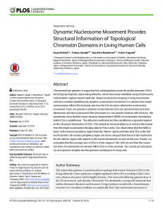
model can predict the trajectory, especially the COM trajectory, during STS movement. 2. METHOD 2.1. Data Acquisition Five university students (20and 25 years) without neurological or musculoskeletal disorders volunteered to participate to this study. All subjects gave informed consent. They were asked to perform three types of STS movements with their arms crossed over their chest, i.e., natural (NT), leaning-forward (LF), and upright (UP) movement conditions, from a given seated position. The initial posture was set to be 10 [deg] dorsiflexion of the ankle, 90 [deg] flexion of the knee, and 80 [deg] flexion of the hip. In the NT condition, the subjects were instructed to stand up at natural speed. In the LF condition, they were told to stand with leaning trunk forward deeply at the beginning of the movement. In the UR condition, the subjects were told to stand without leaning trunk forward. Each subject was told to make fifteen movements for each of the three conditions. The measurement was started by record for the NT condition in each subject. The order of the measurement for the UP and LF conditions was randomly assigned for each subject. Position data of markers placed on the ankle, knee, hip, and shoulder joints were recorded using a 3D motion analysis device (Vicon MX) at a sampling frequency of 200Hz and low-pass filtered at a cut-off frequency of 3 Hz to yield the angular data (Fig. 1.). Also, the vertical force of the seat was measured using a force plate (Kistler 9287B) at a sampling frequency of 1 kHz. 2.2. Data Analysis 2.2.1 Movement time Since the linear velocity of the COM exhibited a bell shaped profile, the onset and termination of the STS movement were determined as the time when the linear velocity of the COM exceeded above and decreased below 5% of its peak, respectively. In addition, the rising time was defined as the time between the seat-of (the moment when

2135

the vertical force of the seat decreased to zero) and the termination of the movement.

of the movement, d is the shortest distance from the instantaneous COM position to the line L. The trajectory convex upward was defined as positive. The maximum and minimum values of the linearity during movement were then obtained for each trial. 2.2.4 Variability of COM position The spatial variability of the COM during movement was evaluated using the value defined by the following equation;

-θ3 Hip θ2

Variability= Knee

Stool

Fig. 1. Definition of the joint angles. θ1: Dorsi-flexion of the ankle, θ2: Flexion of the knee θ3: Flexion of the hip. A positive value indicates angle for clock-wise direction.

2.2.2 Calculation of joint torque, center of mass, and measured costs The joint torque (muscle torque) at the joint and center of mass (COM) of the subject were calculated for the threelinked rigid body model composed of the shank, thigh, and body (head, arm, and trunk). Mass and inertia of the segments were estimated from the weight and height of the subject. The torque change cost was obtained by integrating numeric differentiate of torques using following equation; Torque change cost =

∑ ∑τ i

2 it

(1)

t =t 0

where T indicates the rising time (T=tf-t0), t0 and tf are the time instance of the seat-off and termination of the movement, τ it is torques at the i-th joints at the time of t. Measured jerk cost of COM movement was calculated as follows; 1 Jerk cost = 5 T

∑ (x

t

+ yt ) 2

1 n

∑(y n

ti

− yt ) 2

(4)

i =1

2.3.1. Minimum jerk trajectory for COM. The minimum Cartesian jerk trajectory for COM was obtained by minimizing the following cost function; Cj=

1 2

∫ (x tf

+y 2 ) dt

(5)

x(t ) = x0 + ( x f − x0 )(10τ 3 − 15τ 4 + 6τ 5 ) + Tv x 0 (τ − 10τ 3 + 15τ 4 − 6τ 5 ) + T (v xf − v x 0 )(−4τ 3 + 7τ 4 − 3τ 5 )

(6)

2

T a x 0 (τ 2 − 2τ 3 + τ 4 ) 2 T2 + ( a xf − a x 0 )(τ 3 − 2τ 4 + τ 5 ) 2 y (t ) = y 0 + ( y f − y 0 )(10τ 3 − 15τ 4 + 6τ 5 )

(2)

+

t =t 0

where T is the rising time (T=tf-t0), x and y are the horizontal and vertical position of the COM, respectively. The cost was normalized by T5 corresponding to the highest order of polynomial equation for the minimum jerk trajectory (see equation (6) and (7)).

+ Tv y 0 (τ − 10τ 3 + 15τ 4 − 6τ 5 ) + T (v yf − v y 0 )(−4τ 3 + 7τ 4 − 3τ 5 )

2.2.3 Linearity of COM trajectory

(7)

2

T a y 0 (τ 2 − 2τ 3 + τ 4 ) 2 T2 ( a yf − a y 0 )(τ 3 − 2τ 4 + τ 5 ) + 2 +

Linearity of the COM trajectory during the rising time in Cartesian coordinates was quantified by the equation as follows; Linearity = d/L (3) where L is the length of line connecting the COM positions at the instance of the seat-off and the termination

2

t =t 0

where x and y denote the position of COM in the Cartesian coordinates. Applying the method of variational calculus, we can obtain an optimal trajectory of COM analytically as,

tf

2

i =1

( xti − xt ) 2 +

2.3. Simulation For each subject and condition, average position, velocity, and acceleration data at the seat-off and termination of the movement were given as initial and final boundary conditions to compute the minimum jerk and the minimum torque-change trajectories.

tf

1 T

∑ n

where n is the total number of trials (n=15), xti and yti are the horizontal and vertical position of COM at the time of t in the i-th trial. Also, x t and y t are the averaged horizontal and vertical position of COM at the time of t, respectively. Since the movement times were different from trial to trial, the movement time was normalized to 1, the values of variability were calculated for 100 points which equally divide the normalized movement time.

Ankle

θ1

1 n

where, xo and y0, are the position, vx0,and vy0 are velocity, ax0 and ay0 are acceleration of the COM at the seat-off for the horizontal and vertical direction, respectively, and xf , yf, vxf, vyf, axf, and ayf are those at the termination of the

2136

Figure 2. Profiles of angular and torque data in the upright condition (UP). Data from a subject. Dotted lines: experimental data, Thick line: Prediction of the minimum torque change model.

movement. τ denotes time sequence normalized with the rising time T=tf-t0, i.e., the time from the seat-off to termination of the movement. 2.3.2. Minimum torque- change trajectory. The objective cost function CT was defined as follows; CT =

1 2

T

3

0

i =1

∫∑

 dτ i   dt

2

  dt 

each subject with zero-viscous parameters. Using the methods of dynamic programming and variational calculus, the optimization problem results in a two-point boundary value problem of the set of nonlinear ordinary differential equations [6]. For each subject and condition, the boundary conditions were set separately according to each subject’s averaged data.

(8)

3. RESULTS

where τ i is the torque at the i-th joint out of three joints. To calculate minimum torque-change trajectory, dynamics of the body must be specified. In this paper, we adopted, as the body model, a three-link rigid body whose link parameters corresponds to the anthropometric size of

3.1. Movement time The averaged movement times for the upright (UP), natural (NT), and lean-forward (LF) conditions across five subjects were 1.07 +/- 0.03 sec, 1.07 +/- 0.02 sec, and 1.12

Table. 1. Averaged values at the seat-off and the termination of the STS movement. (n=5.) Angle (rad) Angular velocity (rad/s) Torque (Nm) UP NT LF UP NT LF UP NT LF Ankle 1.29 1.33 1.33 -0.54 -0.45 -0.45 -60.67 -50.09 -20.35 (0.045) (0.034) (0.027) (0.263) (0.149) (0.092) (23.51) (11.29) (25.00) Knee 1.29 1.28 1.26 -0.624 -0.639 -0.461 -126.3 -106.4 -74.74 Seat-off (0.075) (0.082) (0.062) (0.278) (0.246) (0.083) (21.77) (14.92) (26.66) Hip 59.71 79.88 100.3 -1.45 -1.73 -2.09 1.31 0.76 0.088 (0.040) (0.087) (0.070) (0.529) (0.147) (0.535) (16.91) (26.45) (26.97) Ankle 1.41 1.38 1.36 0.0038 -0.022 0.0089 37.29 53.01 54.98 (0.024) (0.043) (0.027) (0.064) (0.031) (0.075) (15.12) (20.41) (22.80) Knee 1.18 1.17 1.18 -0.093 -0.068 -0.203 -1.29 7.52 10.95 Termination (0.059) (0.088) (0.057) (0.136) (0.082) (0.134) (7.104) (11.00) (13.33) Hip -0.0044 0.021 -0.066 0.107 -0.118 -0.042 3.95 0.183 0.560 (0.105) (0.090) (0.104) (0.074) (2.44) (3.61) (0.121) (0.171) (6.16) Mean (standard deviation)

2137

+/- 0.02 sec, respectively. In average, the movement time for LF was longer than the UP and NT conditions, whereas the movement time for UP was comparable with that of NT. 3.2. Joint kinematics and torque magnitude at the seat-off and the termination of the movement. Figure 2 shows the angle, angular velocity, torque, and torque change for a subject during UP condition. Trajectories for all trials and the optimized data were superimposed. The trajectories predicted by the minimum torque-change model were found to be quite similar to the experimental data also in the NT and LF conditions. Averaged angles, angular velocities, and torques at the seat-off and the termination across subjects were shown in Table. 1. The flexion angle of the hip joint at the seat-off in the LF condition was greater than NT and UP condition, and flexion angle of the hip in the NT was greater than UP condition. Also, the extension angular velocity of the hip at the seat-off in the UP condition was larger than NT, and that in the NT was larger than LF. It was confirmed that the subjects performed different STS movements according to the instruction from the experimenter. Comparing the averaged torque magnitudes at seat-off, extension torques at the ankle and knee joints in the UP condition were greater than those in NT and LF conditions, while the extension torque of the hip joint was greatest in the LF condition. These results show that the UR condition required greater extension torque at the knee and ankle joints in order to lift the body. At the termination of the movement, all subjects stood steadily. There were no significant differences in the final posture between the conditions except for the angular velocities of the hip joint. 3.3 Variability of COM position Figure 3 shows the spatial variability of the COM at the initial position, the maximum variability, and at the final position for all subjects. The initial and final variability were less than 25 mm. In the natural (NT) condition, the initial variability tended to be slightly greater than that of upright (UP) and lean-forward (LF) conditions for three subjects. Also, the final variability in the NT condition tended to be greater than UP and LF conditions except for a subject. A weak correlation was found between the initial and final variability (r=0.57, p=0.02). The maximum variability was less than 75 mm. There was no consistent relationship between the initial variability and the maximum variability (r=0.14, p=0.60), and between the maximum and final variability (r=0.30, p=0.26).

Figure 3. The initial (upper panel), maximum (middle panel), and final (lower panel) variability of the center of mass (COM). Data for all subjects. UP: upright condition, NT: natural condition, LF: lean-forward condition.

3.4 Linearity of the COM trajectory The averaged maximum and minimum linearity and the timing of occurrence of the maximum and minimum linearity across subjects were summarized in Table. 2. The linearity and timings predicted by the models are shown as well. A positive value of the linearity indicates the trajectory was convex upward. Values in the timing indicate percent of time from the seat-off to termination of the movement. In the leaning-forward (LF) condition, the trajectory of the COM convex downwardly and timing of occurrence of maximum and minimum were delayed compared to the upright (UP) and natural (NT) condition. These trends in linearity and timings in different conditions were predicted

Table. 2. Maximum and minimum linearity index and timing of its occurrence. Measured MJ Linearity Timing (%) Linearity Timing (%) UP 0.079 (0.0006) 48.4 (0.39) 0.036 (0.019) 59.7 (9.4) Max NT 0.084 (0.001) 50.9 (0.4) 0.036 (0.018) 61.6 (9.8) LF 0.031 (0.0008) 75.2 (4.0) 0.008 (0.001) 86.2 (13.8) UP -0.016 (0.0002) 14.2 (0.8) -0.017 (0.017) 10.8 (6.7) Min NT -0.017 (0.0001) 9.3 (0.1) -0.02 (0.016) 13.0 (6.3) LF -0.097 (0.005) 20.0 (0.5) -0.115 (0.098) 25.6 (6.7) Mean (standard deviation)

2138

MTC Linearity Timing (%) 0.076 (0.063) 53.5 (13.6) 0.087 (0.05) 51.1 (8.4) 0.026 (0.038) 75.4 (17.4) -0.018 (0.016) 10.3 (6.2) -0.018 (0.013) 10.0 (4.4) -0.099(0.085) 20.9 (6.5)

Figure 4. Trajectory of the center of mass (COM) in the natural condition (NT). Data from a subject. Dotted lines: experimental data, Black thick line: Prediction of the minimum torque-change model, Gray thick line: Prediction of the minimum jerk model.

by both the MJ and MTC. In average, the maximum linearity indexes predicted by the MJ were larger than measured linearity index in each condition, also the timing predicted by MJ were delayed greatly to the measured timings in most of the trials. On the other hand, prediction of the MTC was comparable with the measured linearity indexes and the timings.

3.4. Peak velocity of the COM Figure 4 shows the example of position, velocity, and acceleration profiles of the COM of a subject after the seatoff in the natural (NT) condition. Trajectories of fifteen trials and predictions from the minimum jerk (MJ) and minimum torque-change (MTC) were superimposed. Since horizontal peak velocity was observed before the seat-off in almost trials, magnitude of vertical peak velocity and timing were analyzed. It is observed that vertical peak velocity of the minimum jerk model was smaller than that of the minimum torque-change model and experimental data. Table 3 summarized the averaged peak velocity and its timings for all subject. MTC prediction of peak velocity was comparable with the measured peak velocity in average. The time to vertical peak velocity (TPV) of the COM predicted by MTC was comparable with the measured TPV. In addition, both model predicted that the TPV in the LF condition was delayed to NT and UP conditions. In sum, the

predictions of MTC model resembled the measured features of the COM trajectories. 3.5. Costs for the rising Figure 5 shows measured jerk cost and measured torque change cost for three movement patterns. In the upright (UP) condition, both costs exhibited significantly greater value than in the natural (NT) and leaning-forward (LF) conditions (F2, 222=6.407, p