The Efficiency of Artificial Neural Networks for Forecasting in the ...

International Journal of Statistics and Probability; Vol. 5, No. 2; 2016 ISSN 1927-7032 E-ISSN 1927-7040 Published by Canadian Center of Science and Education

The Efficiency of Artificial Neural Networks for Forecasting in the Presence of Autocorrelated Disturbances Alexander K White1 & Samir K Safi1,2 1

Texas State University, San Marcos, Texas, USA.

2

The Islamic University of Gaza, Palestine

Correspondence: Samir K Safi, Texas State University, San Marcos, Texas, USA. [email protected] Received: January 22, 2016 doi:10.5539/ijsp.v5n2p51

Accepted: February 10, 2016

Online Published: February 14, 2016

URL: http://dx.doi.org/10.5539/ijsp.v5n2p51

Abstract We compare three forecasting methods, Artificial Neural Networks (ANNs), Autoregressive Integrated Moving Average (ARIMA) and Regression models. Using computer simulations, the major finding reveals that in the presence of autocorrelated errors ANNs perform favorably compared to ARIMA and regression for nonlinear models. The model accuracy for ANN is evaluated by comparing the simulated forecast results with the real data for unemployment in Palestine which were found to be in excellent agreement. Keywords: Artificial Neural Networks, Time Series, Regression 1. Introduction A good forecasting model is a key component to proper planning. Many different approaches exist for developing the forecast model, each designed to address special situations which arise in the time series. In this paper, we compare two traditional methods: Linear Regression and Autoregressive Integrated Moving Average to Artificial Neural Networks (ANNs). Given the complex contexts in which time series arise, there is a need for robust forecasting model which is flexible enough to be of use in a variety of situations. Previous research indicates that ANNs may provide such approach, see for example (Potočnik, et al. 2015, Adhikari & Agrawal, 2014, Thielbar & Dickey, 2011, Khashei & Bijari, 2010, Aksoy & Dahamsheh, 2009, Yasdi, 1999, among many others). Neural networks are the preferred tool for many predictive data mining applications because of their flexibility, power, accuracy and ease of use. The statistical methods assume that data are linearly related and therefore is not true in real life applications. The newly introduced method, the ANN which is inherently a nonlinear network and does not make such assumption, therefore is well suited for prediction purpose. (Safi, 2013). We use a data set of unemployment rates from Palestinian Central Bureau of Statistics (PCBS). The dataset contains the quarterly unemployment rates in Palestine during the period of the first quarter of 2000 through the second quarter of 2015. R-statistical software is used for fitting ANN, ARIMA, and regression models for the unemployment rates time series data. In this paper, ANN, ARIMA and regression models have been conducted for unemployment rates forecasting in Palestine. The main purpose of this paper is to find a more accurate and reliable forecasting model for the unemployment rates in Palestine. This paper is organized as follows: Section 2 presents review of ANN literature; in section 3, we present the comprehensive computer simulation results. Section 4 displays three forecasting cases fitting ARIMA, ANN, and Regression models for unemployment data in Palestine; and section 5 concludes some important results of this paper and offers future research. 2. Review of ANN Literature Artificial neural networks (ANN) have received a great deal of attention over the last years. They are being used in the areas of prediction and classification, areas where regression and other related statistical techniques have traditionally been used. (Cheng & Titterington, 1994). Box, et al. (1995) have developed the integrated autoregressive moving average (ARIMA) methodology for fitting a class of linear time series models. However, the statistical methods assume that data are linearly related and which is typically not true in real life applications. The newly introduced method, ANN, has emerged to be popular as it does not make such assumptions. The ANN, which is inherently a nonlinear network and does not make such assumptions, is

51

www.ccsenet.org/ijsp

International Journal of Statistics and Probability

Vol. 5, No. 2; 2016

well suited for prediction purposes. Kohzadi, et al. (1996) compared neural network and ARIMA models to forecast US monthly live cattle and wheat cash prices. Results showed the neural network forecasts were considerably more accurate than those of the traditional ARIMA models, which were used as a benchmark. Szkuta, et al. (1999) presented the System Marginal Price (SMP) short-term forecasting implementation using the Artificial Neural Networks (ANN) computing technique. The main results presented in their paper confirm considerable value of the ANN based approach in forecasting the SMP. ANNs constitute one of the most powerful tools for pattern classification due to their nonlinear and non-parametric adaptive-learning properties. Many studies have been conducted that have compared ANNs with other traditional classification techniques, since the default prediction accuracies of ANNs are better than those using classic linear discriminant analysis and logistic regression techniques, see for example Lee & Chen (2005) and Lee, et al. (2002). Allende, et al. (2002) showed that ANN is a superior technique in the modeling non-linear time series such as: bilinear models, threshold autorregressive models and regression trees. If the functional form linking inputs and output is unknown, only known to be extremely complex, or of no interest to the investigator, an analysis using ANN may be best. The availability of large training datasets and powerful computing facilities are requirements for this approach. In addition, if a non-linear relationship exists between inputs and outputs, then data of this complexity may best modeled by an ANN. Zhang (2003) presented a combining approach to time series forecasting. The linear ARIMA model and the nonlinear ANN model are used jointly, aiming to capture different forms of relationship in the time series data. The hybrid model takes advantage of the unique strength of ARIMA and ANN in linear and nonlinear modeling. For complex problems that have both linear and nonlinear correlation structures, the combination method can be an effective way to improve forecasting performance. The empirical results clearly suggest that the hybrid model is able to outperform each component model used in isolation. Gheyas & Smith (2009) proposed Generalized Regression Neural Networks (GRNN) for forecasting univariate time series. They compared GRNN ensemble with existing algorithms (ARIMA & GARCH, MLP, GRNN with a single predictor and GRNN with multiple predictors) on forty datasets. The one-step process is iterated to obtain predictions ten-steps-ahead. The results obtained from the experiments show that the GRNN ensemble is superior to existing algorithms. The existence of good model to forecast is very crucial for policy makers. Good policy requires that first identification of relationship for data (linear or non-linear). Artificial Neural Networks have been successfully used in a variety of areas. Research evidence shows that for any system with non-linear instability patterns such as the market for housing, the utilization of the ANN methodology serve properly (Bahramianfar, 2015). Valipour, et al. (2013) showed that by comparing root mean square error (RMSE) and mean bias error (MBE), dynamic artificial neural network model was chosen as the best model for forecasting inflow of the Dez dam reservoir. KÖLMEK & Navruz (2015) constructed simulation studies about price modeling via artificial neural networks and proper artificial neural network configurations. They showed that the neural network model gave better results over a time-series model. Potočnik, et al. (2015) showed that neural network models exhibited the overall best forecasting performance, and suggested that neural network (NN) or the neural network models with a direct linear link (NNLL) structures should be considered as forecasting solutions for applied forecasting in district heating markets. 3. Simulation Study 3.1 The Simulation Setup In this section, we present a computer simulation comparing the robustness of three forecasting techniques: ANNs, ARIMA, and Regression. These simulations examine the sensitivity of forecasting approaches to model misspecification. The efficiency of the approaches are compared using the root mean squared forecast error (RMSFE) of the ANNs model relative to ARIMA and regression models. Time series were generated of the form:

Yt  f (t )   t , 𝜀𝑡 = 𝜙𝜀𝑡−1 + 𝑢𝑡 , t=1,…,T

(1)

The errors follow a first order autoregressive AR(1) model with coefficient 0 < 𝜙 < 1 and 𝑢𝑡 independent standard normal. Eighteen cases are considered in the results shown below: three finite series lengths (T = 20, 50, and 100), two

52

www.ccsenet.org/ijsp

International Journal of Statistics and Probability

Vol. 5, No. 2; 2016

choices of the linking function f (S-curve and linear) and three autoregressive coefficients For each case, 1000 series were generated.

  0.1, 0.5, 0.9 

are used.

In this simulation, we used AR(1), because most of the time in the economic time series, data generating processes is explainable in terms of autoregressive of order one or two. The most commonly assumed process in both theoretical and empirical studies is the first-order autoregressive process or briefly, AR(1). At one time, the AR(1) process was the only autocorrelation process considered by economists. Most economic data series were annual, for which the AR(1) process is reasonable. This may explain the wide use of this process, as estimation of other more complicated processes is not manageable without the aid of a computer (Safi & White, 2006). We introduce definitions of the simulation RMSFE, the relative efficiency, and the two selected models of dependent variable. Definition 1: The simulation RMSFE is a measure of the size of the forecast error, that is, the magnitude of a typical mistake made using a forecasting model. The RMSFE is given by



RMSFE  E  YT 1  YˆT 1|T 

  , 2

where YˆT 1|T is the forecast of YT 1 based on information through period T , using a model estimated with data through period T (Stock & Watson, 2015). Definition 2: The efficiency of the ANNs forecasts relative to that of ARIMA in terms of the simulation RMSFE,

ˆ 

 E  Y 

   

E  YT 1  YˆT 1|T  T 1

 YˆT 1|T

ˆ is given by

2

ANN

2

ARIMA

A ratio less than one indicates that the ANNs forecast is more efficient than ARIMA, and if ˆ is close to one, then the ANNs forecast is nearly as efficient as ARIMA forecasts. Otherwise, ANNs performs poorly, (Safi, 2016). Definition 3: The models used in the simulation are defined below. The S-curve model:

f  t   exp  b0  b1t 1 

The Linear model: f  t   b0  b1t The model coefficients b0 , and b1 were each chosen to be equal one, respectively. 3.2 Simulation Results We discuss the simulation results based on the ratio of the estimated RMSFE of ANNs to that of ARIMA and regression. Table 1 shows the complete simulation results for the ratios of RMSFE of ANNs to that of ARIMA and regression for the two different models, all selected sample sizes and autocorrelation coefficients. Table 1. Ratios of RMSFE for ANN to ARIMA and Regression

  0.1 20 Model S-curve Linear

ANN/ARIMA 0.8822 2.2491

ANN/REG 0.6074 0.1440

S-curve Linear

0.9633 1.9286

0.6890 0.1349

S-curve Linear

1.2373 1.8612

0.6570 0.1407

50 ANN/ARIMA ANN/REG 0.9406 0.8217 3.9681 0.0947   0.5 0.9886 0.8976 3.2729 0.0907   0.9 0.9952 0.7082 2.3330 0.0941

53

100 ANN/ARIMA ANN/REG 0.9984 0.9328 30.3245 0.3474 1.0039 25.4987

0.9536 0.3509

0.9760 14.7658

0.8392 0.3530

www.ccsenet.org/ijsp

A)

B)

International Journal of Statistics and Probability

Vol. 5, No. 2; 2016

For Non-Linear Model (S-curve) - ANNs perform more efficiently than ARIMA and regression for the S-curve for all selected sample sizes and autocorrelation coefficient,   0.1 . For example, o For n  20 , the relative efficiencies of ANNs to ARIMA and regression equal ˆ  0.8822, 0.6074 , respectively. This result indicates that RMSFEs for ANNs equal 88.22% and 60.74% of that of ARIMA and regression models, respectively. Therefore, ANNs superior on ARIMA and regression for small sample size and   0.1 . o For n  50 , the relative efficiencies of ANNs to ARIMA and regression equal ˆ  0.9406, 0.8217 , respectively. This result indicates that RMSFEs for ANNs equal 94.06% and 82.17% of that of ARIMA and regression models, respectively. Hence, ANNs is more efficient than ARIMA and regression for moderate sample size and   0.1 . o For n  100 , the relative efficiencies of ANNs to ARIMA and regression equal ˆ  0.9984, 0.9328 , respectively. This result indicates that RMSFEs for ANNs equal 99.84% and 93.28% of that of ARIMA and regression models, respectively. Hence, ANNs perform nearly as efficiently as ARIMA and regression models for large sample size and   0.1 . - ANNs perform nearly as efficiently as ARIMA and more efficient than regression for the S-curve for all selected sample sizes and autocorrelation coefficients,   0.5 and 0.9 . For example, o For n  20 , the relative efficiencies of ANNs to ARIMA and regression equal ˆ  0.9633, 0.6890 , respectively. This result indicates that RMSFEs for ANNs equal 96.33% and 68.90% of that of ARIMA and regression models, respectively. Therefore, ANNs perform nearly as efficiently as ARIMA and are superior to regression for small sample size and   0.5 . o For n  50 , the relative efficiencies of ANNs to ARIMA and regression equal ˆ  0.9952, 0.7082 , respectively. This result indicates that RMSFEs for ANNs equal 99.52% and 70.82% of that of ARIMA and regression models, respectively. Hence, ANNs perform nearly as efficiently as ARIMA and more efficient than regression for moderate sample size and   0.9 . o For n  100 , the relative efficiencies of ANNs to ARIMA and regression equal ˆ  0.9760, 0.8392 , respectively. This result indicates that RMSFEs for ANNs equal 97.60% and 83.92% of that of ARIMA and regression models, respectively. Hence, ANNs perform nearly as efficiently as ARIMA and more efficient than regression for large sample size and   0.9 . - We notice, there is a situation where ANNs performs poorly compared to ARIMA. When n  20 and   0.9 , the relative efficiency of ANNs to ARIMA equals ˆ  1.2373 . This result indicates that RMSFE for ANNs is 23.73% more than that for ARIMA. For Linear Model ANNs perform poorly compared to ARIMA, but are superior to regression for the linear model for all selected sample sizes and autocorrelation coefficients. For example, - For n  20 and   0.1 , the relative efficiencies of ANNs to ARIMA and regression equal ˆ  2.2491, 0.1440 , respectively. This result indicates that RMSFEs for ANNs equal 224.91% and 14.40% of that of ARIMA and regression models, respectively. - For n  50 and   0.5 , the relative efficiencies of ANNs to ARIMA and regression equal ˆ  3.2729, 0.0907 , respectively. This result indicates that RMSFEs for ANNs equal 327.29% and 9.07% of that of ARIMA and regression models, respectively. - For n  100 and   0.9 , the relative efficiencies of ANNs to ARIMA and regression equal ˆ  14.7658, 0.3530 , respectively. This result indicates that RMSFEs for ANNs equal 1476.58% and 35.30% of that of ARIMA and regression models, respectively.

3.3 Summary For non-linear model, ANNs were more efficient than ARIMA for all selected sample sizes and   0.1 . While, ANNs perform nearly as efficiently as ARIMA for all selected sample sizes and   0.5 , 0.9 . However, ANNs performs poorly as efficiently compared to ARIMA when n  20 and   0.9 . In addition, ANNs were more efficient than regression for all selected sample sizes and autocorrelation coefficients. For linear model, ANNs perform poorly compared to ARIMA, but were superior to regression for all selected sample sizes and autocorrelation coefficients. 4. Fitting Models for unemployment Data This section presents the fitting models for unemployment rates data by using three different approaches, ANN, ARIMA(p,d,q), and regression models. Consider the quarterly unemployment in Palestine, from the first quarter in 2000

54

www.ccsenet.org/ijsp

International Journal of Statistics and Probability

Vol. 5, No. 2; 2016

25 20 10

15

Unemployment Rates

30

35

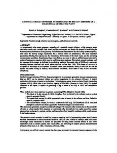
through the second quarter 2015, Figure 1 displays the time series plot. The series displays considerable fluctuations over time, especially in 2000 and 2003, and a stationary model does not seem to be reasonable. The higher values display considerably more variation than the lower values.

2000

2005

2010

2015

Years

Figure 1. Unemployment Rates in Palestine: 2000:Q1 – 2015:Q2 The forecasting results are presented in the following sub-sections. 4.1 Fitting ANN Model for Unemployment Data Applying ANN with average of 20 networks, each of which is a 1-1-1 network. R-software is used for fitting ANN model for the time series. Some commands and functions with input and output variables have been used. The nnetar function is used to fit neural networks (Venables & Ripley, 2002). The estimated noise variance is  e2  5.587 . RMSFE is used as stopping criteria in the network. Smaller values of RMSFE indicate higher accuracy in forecasting. The Neural network result shows that the minimum RMSFE equals 2.3636. 4.2 Fitting ARIMA Model for Unemployment Data We use maximum likelihood estimation and show the results obtained from auto.arima command by using the R statistical software in Table 1. Here we see that ˆ  0.6980 . We also see that the estimated noise variance is ˆ e2 =10.91 . Noting the P-value, the estimate of autoregressive is significantly different from zero statistically, as is the intercept term. Table 2. Maximum Likelihood Estimates from R Software: Unemployment Rates Coefficients

AR(1) Intercept* 0.6980 23.7062 SE 0.1006 1.3543 T 6.9384 17.5044 P-value < 0.0001 < 0.0001 * The intercept here is the estimate of the process mean  not of 0 The estimated model can be written

Yt  23.7062  0.6980 Yt 1  23.7062  The intercept of ARIMA is  0   1     23.7062 1  0.6980   7.1593 . Therefore, the estimated model is

Yt  7.1593  0.6980Yt 1

(2)

The AR(1) result shows that the RMSFE equals 3.3034. 4.3 Fitting Regression Model for Unemployment Data The estimated linear regression model in (3) is obtained by using the Ordinary Least Square (OLS) estimation method;

55

www.ccsenet.org/ijsp

International Journal of Statistics and Probability

Vol. 5, No. 2; 2016

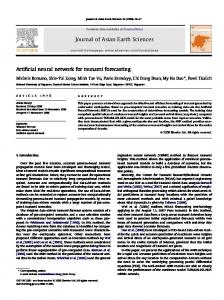
YT  23.76399  0.01205 T , (3) 2 where T is the time. We also see that the estimated noise variance is  e  19.8035 . The regression result shows that the RMSFE equals 4.3777. Table 3 and Figure 2 show the forecasting results for unemployment through 2015: Q3-2017:Q4 based on ANN and ARIMA(1,0,0), and regression models. Table 3. Forecasting results of ANN, ARIMA and Regression Models for Unemployment Year ANN ARIMA Regression 2015:Q3 27.24513 24.46972 24.52311 2015:Q4 25.82734 24.23918 24.53516 2016:Q1 25.30061 24.07825 24.54721 2016:Q2 24.87816 23.96592 24.55926 2016:Q3 26.25636 23.8875 24.57131 2016:Q4 25.43741 23.83277 24.58336 2017:Q1 25.1259 23.79456 24.59541 2017:Q2 24.90719 23.76789 24.60746 2017:Q3 25.68694 23.74928 24.61951 2017:Q4 25.20924 23.73628 24.63156 The RMSFE for forecasting using ANN, ARIMA, and regression equal 2.3636, 3.3034, and 4.377747, respectively. This result shows that RMSFE of ANN is 71.55% and 53.99% of RMSFE for ARIMA and regression, respectively. So RMSFE forecasting of ANN is the smaller than that by using ARIMA and regression models. This means ANN model for forecasting is more accurate and efficient than the ARIMA, and regression forecasting models.

25 20 10

15

Unemployment

30

35

Forecasting for Unemployment Rates by ANN

2000

2005

2010

2015

Years

25 20 15 10

Unemployment

30

35

Forecasting for Unemployment Rates by ARIMA

2000

2005

2010 Years

56

2015

www.ccsenet.org/ijsp

International Journal of Statistics and Probability

Vol. 5, No. 2; 2016

25 20 10

15

Unemployment

30

35

Forecasting for Unemployment Rates by Regression

0

10

20

30

40

50

60

Time

Figure 2. Forecasting results of ANN, ARIMA and Regression Models for Unemployment Rates 5. Conclusion and Future Research In this paper, we show that Artificial Neural Networks provide a good alternative to traditional approaches for fitting time series. In the simulation results for time series with autocorrelated errors, the ANN approach was much more efficient than regression in forecasting future observations of the time series. When compared to ARIMA, ANNs performed well when the linking function was nonlinear, outperforming ARIMA in 7 of the 9 cases and nearly the same in 1 of the two remaining cases. However, when the linking function was linear, ARIMA outperformed ANN. This is not surprising since ARIMA is designed to fit this particular situation. It is interesting to note, however, that the difference in performance was smaller when ϕ is close to 1. All three approaches were used to forecast the unemployment in Palestine. The regression model predicts a nearly constant unemployment rate for the next 10 quarters. The fit of the regression line was poor. Comparing the ANN and the ARIMA model, we see considerable differences. The ANN model forecasts exhibit more short term variation than the ARIMA model. The RMSFE indicates that the ANN provides a better fit to the data. Taken, together this shows that ANN is the preferable approach for this data set. The models studied here were restricted to univariate time series. In the context of economic forecasting there are typically many correlated time series available for analysis. One avenue for future investigation, is to use ANNs in the context of multivariate time series to forecast multiple time series simultaneously. Another, is investigate the effectiveness of ANNs to model data where seasonality is known to exist. Acknowledgment We would like to express the deepest appreciation to Dr. Saif El-Dean Ouda, Department of research and monetary policy, Palestinian Monetary Authority (PMA) for providing us with the data set. Also, we are grateful for the referees for their valuable comments, suggestions, and review on earlier draft of this paper. References Adhikari, R., & Agrawal, R. K. (2014). A combination of artificial neural network and random walk models for financial time series forecasting. Neural Computing and Applications, 24(6), 1441-1449. http://dx.doi.org/10.1007/s00521-013-1386y Aksoy, H., & Dahamsheh, A. (2009). Artificial neural network models for forecasting monthly precipitation in Jordan. Stochastic Environmental Research and Risk Assessment, 23(7), 917-931. http://dx.doi.org/10.1007/s00477-008-0267-x. Allende, H., Moraga, C., & Salas, R. (2002). Artificial neural networks in time series forecasting: A comparative analysis. Kybernetika, 38(6), 685-707. Bahramianfar, P. (2015). Forecasting US Home Prices with Neural Network and Fuzzy Methods. LAP LAMBERT Academic Publishing, Germany. Box, G. E. P., Jenkins, G. M., & Reinsel, G. C. (1995). Time series analysis forecasting and control, Third Edition. New Jersey: Prentice Hall.

57

www.ccsenet.org/ijsp

International Journal of Statistics and Probability

Vol. 5, No. 2; 2016

Cheng, B., & Titterington, D. M. (1994). Neural networks: A review from a statistical perspective. Statistical science, 2-30. ISSN: 08834237. Gheyas, I. A., & Smith, L. S. (2009). A neural network approach to time series forecasting. In Proceedings of the World Congress on Engineering, 2, 1-3. ISBN: 978-988-18210-1-0. Khashei, M., & Bijari, M. (2010). An artificial neural network (p, d, q) model for time series forecasting. Expert Systems with applications, 37(1), 479-489. http://dx.doi.org/10.1016/j.eswa.2009.05.044. Kohzadi, N., Boyd, M. S., Kermanshahi, B., & Kaastra, I. (1996). A comparison of artificial neural network and time series models for forecasting commodity prices. Neurocomputing, 10(2), 169-181. http://dx.doi.org/10.1016/0925-2312(95)00020-8. KÖLMEK, M. A., & Navruz, I. (2015). Forecasting the day-ahead price in electricity balancing and settlement market of Turkey by using artificial neural networks. Turkish Journal of Electrical Engineering & Computer Sciences, 23(3). http://dx.doi.org/10.3906/elk-1212-136. Lee, T. S., & Chen, I. F. (2005). A two-stage hybrid credit scoring model using artificial neural networks and multivariate adaptive regression splines. Expert Systems with Applications, 28(4), 743–752. http://dx.doi.org/10.1016/j.eswa.2004.12.031. Lee, T. S., Chiu, C. C., Lu, C. J., & Chen, I. F. (2002). Credit scoring using the hybrid neural discriminant technique. Expert Systems with Applications, 23(3), 245–254. http://dx.doi.org/10.1016/S0957-4174(02)00044-1. Potočnik, P., Strmčnik, E., & Govekar, E. (2015). Linear and Neural Network-based Models for Short-Term Heat Load Forecasting. Journal of Mechanical Engineering, 61(9), 543-550. http://dx.doi.org/10.5545/sv-jme.2015.2548. Safi, S. (2016). A Comparison of Artificial Neural Network and Time Series Models for Forecasting GDP in Palestine. American Journal of Theoretical and Applied Statistics, 5(2), 58-63. http://dx.doi.org/10.11648/j.ajtas.20160502.13 Safi, S. K. (2013). Artificial Neural Networks Approach to Time Series Forecasting for Electricity Consumption in Gaza Strip. IUG Journal of Natural and Engineering Studies, 21(2), 1-22. ISSN 1726-6807. Safi, S., & White, A. (2006). The Efficiency of OLS In The Presence Of Auto-Correlated Disturbances in Regression Models. Journal of Modern Applied Statistical Methods, 5(1), 10. ISSN: 1538-9472. Stock, J., & Watson, M. (2015). Introduction to Econometrics. Updated third edition. Prentice Hall. Szkuta, B. R., Sanabria, L. A., & Dillon, T. S. (1999). Electricity price short-term forecasting using artificial neural networks. Power Systems, IEEE Transactions on, 14(3), 851-857. http://dx.doi.org/10.1109/59.780895. Thielbar, M. F., & Dickey, D. A. (2011). Neural Networks for Time Series Forecasting: Practical Implications of Theoretical Results. North Carolina State University. Valipour, M., Banihabib, M. E., & Behbahani, S. M. R. (2013). Comparison of the ARMA, ARIMA, and the autoregressive artificial neural network models in forecasting the monthly inflow of Dez dam reservoir. Journal of Hydrology, 433-441. http://dx.doi.org/10.1016/j.jhydrol.2012.11.017. Yasdi, R. (1999). Prediction of road traffic using a neural network approach. Neural computing & applications, 8(2), 135-142. ISSN: 0941-0643. Zhang, G. P. (2003). Time series forecasting using a hybrid ARIMA and neural network model. Neurocomputing, 50, 159-175. http://dx.doi.org/10.1016/S0925-2312(01)00702-0.

Copyrights Copyright for this article is retained by the author(s), with first publication rights granted to the journal. This is an open-access article distributed under the terms and conditions of the Creative Commons Attribution license (http://creativecommons.org/licenses/by/3.0/).

58