Submitted to: European Symposium on Artificial Neural Networks 2003
Universiteit van Amsterdam
IAS technical report IAS-UVA-02-03
The Generative Self-Organizing Map A Probabilistic Generalization of Kohonen’s SOM J.J. Verbeek, N. Vlassis, and B.J.A. Kr¨ ose Intelligent Autonomous Systems, University of Amsterdam The Netherlands
We present a variational Expectation-Maximization algorithm to learn probabilistic mixture models. The algorithm is similar to Kohonen’s Self-Organizing Map algorithm and can be applied on any mixture model for which we can find a standard Expectation Maximization algorithm. We maximize the variational freeenergy which sums data log-likelihood and Kullback-Leibler divergence between the neighborhood function and the posterior distribution on the components, given data. We illustrate the algorithm with an application on word clustering. Keywords: self-organizing map, Gaussian mixture, free-energy minimization, Expectation-Maximization algorithm, vector quantization.
IAS
intelligent autonomous systems
The Generative Self-Organizing Map
Contents
Contents 1 Introduction
1
2 A simple generative model and EM
1
3 Using free-energy for self-organization
2
4 Discussion
3
5 Illustration
4
6 Conclusions
5
Intelligent Autonomous Systems Informatics Institute, Faculty of Science University of Amsterdam Kruislaan 403, 1098 SJ Amsterdam The Netherlands Tel (fax): +31 20 525 7461 (7490) http://www.science.uva.nl/research/ias/
Corresponding author: J.J. Verbeek tel: +31 20 525 7550
[email protected] http://www.science.uva.nl/~jverbeek/
Copyright IAS, 2002
Section 1 Introduction
1
1
Introduction
Kohonen’s Self-Organizing Map (SOM) [5] is a data analysis method that combines vector quantization with topology preservation. With each quantizer we associate a fixed location in a ‘latent’ space. The latent space is of much lower dimension (typically just two) than the data space. The SOM algorithm finds locations for the quantizers in the data space such that the summed squared distance from data to closest node is small and simultaneously topology is preserved. Topology preservation means that nearby components in latent space are also nearby in the data space. As a consequence, data points associated with nearby components in latent space are coming from similar locations in the data space. Hence, to check if data points are ‘close’ in the data space, we can check whether their associated components are close in the latent space. Topology preservation makes SOMs useful for data visualization and dimensionality reduction. We present a constrained or variational Expectation-Maximization (EM) learning algorithm to learn probabilistic mixture models similar to SOM. The algorithm applies to a wide class of mixture models, in principle to any mixture model for whcih we can find a standard EM algorithm. In the next section we discuss the Gaussian mixture model that will serve as the example mixture model throughout and also briefly discuss the EM algorithm. In section 3 we present our Self-Organizing Mixtures algorithm. We compare our algorithm to several closely related algorithms in Section 4. A brief example application is discussed in Section 5 and we present our conclusions in Section 6.
2
A simple generative model and EM
As generative model consider the Mixture of Gaussians (MoG), given by : k 1X p(x | s), p(x) = k s=1
for D-dimensional data, where p(x|s) is an isotropic Gaussian with inverse variance β and mean µs . Given a data x = {x1 , . . . , xN }, and an initial parameter vector θ = {β, µ1 , . . . , µk } the EM algorithm [6] finds a local maximizer θ of the log-likelihood L(θ). Assuming data are independent and identically distributed: L(θ) =
X n
log p(xn | θ) =
X n
log
1X p(xn | s). k s
Learning is facilitated by introducing a set of N hidden variables. Each hidden variable indicates which of the k mixture components generated the corresponding data point. The EM algorithm maximizes the negative free-energy: F (Q, θ) = EQ log p(x, s; θ) + H(Q) = L(θ) − DKL (Q k p(s | x; θ)),
(1) (2)
where we used H to denote the entropy of a distribution and DKL Qto denote the Kullback-Leibler (KL) divergence between two probability distributions. Q = n qn is a distribution over the hidden variables, qn gives a distribution on the generating mixture component s ∈ {1, . . . , k} for data point n. Note that, due to the non-negativity of the KL-divergence, for any Q, F (Q, θ) is a lower bound on L(θ).
2
The Generative Self-Organizing Map
The two forms in which we expanded F are associated with the M-step and the E-step of EM. In the M-step we change θ as to maximize, or at least increase, F (Q, θ). The first decomposition includes H(Q) which is a constant w.r.t. θ. In the E-step we maximize F w.r.t. Q, the second decomposition includes L(θ) which is constant w.r.t. Q. What remains is a KL divergence which is the effective objective function in the E-step of EM. In standard applications of EM (e.g. mixture modeling) Q is unconstrained, which results in setting qn = p(s | xn ; θ) in the E-step since the non-negative KL divergence equals zero if and only if both arguments are equal. Therefore, after each E-step F (Q, θ) = L(θ). Variational methods are used when optimization over the unconstrained Q is intractable, Q is then restricted to a certain class Q of distributions allowing for tractable computations. Variational EM maximizes F instead of L, the objective sums log-likelihood and a penalty which is high if the true posterior is far from any member of Q.
3
Using free-energy for self-organization
By constraining choosing an appropriate class of distributions Q, we can also enforce a topological ordering between the mixture components, as we explain below. The approach is much like the one taken in [7, 8], where constraints on Q are used to align the local coordinate systems of the components of a probabilistic mixture of factor analyzers. We associate with each mixture component s a latent coordinate gs . It is convenient to take the components as located on a regular grid in the latent space. We set Q to be class of discretized isotropic Gaussians in the latent space, centered on either one of the k component locations gs and with a particular fixed variance. The distributions qn play a similar role as the neighborhood function in Kohonen’s SOM [5]. The qn are thus restricted to be contained in the finite set of distributions Q = {p1 , . . . , pk }, where: exp (−λ k gs − gr k2 ) . pr (s) = P 2 t exp (−λ k gt − gr k )
A small λ corresponds to a broad distribution (high entropy), and for large λ the distribution pr becomes more peaked (low entropy). By performing EM steps, we can never decrease the objective. The M-step is as usual and in the E-step we select for each data point x n the distribution qn ∈ Q that increases the objective the most. Note that in the E-step we can always stick to the qn of the previous EM round without changing (and hence definately not decreasing) the objective funciton. Since the objective function might have local optima and EM is only guaranteed to give locally optimal solutions, good initialization of the parameters of the mixture model is essential to finding a good solution. Analogous to the method of shrinking the extent of the neighborhood function with the SOM, we can start with a small λ (broad neighborhood function) and increase it iteratively until a desired value is reached. In implementations we started with λ such that the p r are close to uniform over the components, then we run the EM algorithm until convergence. Note that if the pr are almost uniform the initialization of θ becomes irrelevant. After convergence we set λnew ← ηλold with η > 1 (typically η is close to unity). In order to initialize the EM procedure with λnew , we initialize θ with the value found in running EM with λold . Using qns = qn (s), for our MoG case F can be rewritten as: F (Q, θ) =
i X h 1 N D log β − qns β k xn − µs k2 /2 + log qns . 2 ns
For fixed λ an EM algorithm can be derived by differentiation:
Section 4 Discussion
3
• E: Determine (by means of exhaustive or sparse search in Q, see below) for each x n the distribution pr∗ ∈ Q that maximizes F , set qn = pr∗ . P P P • M: Set: µs = n qns xn / n qns and β = N D/ ns qns k xn − µs k2 .
The component r ∗ on which pr∗ is centered for data point n, is referred to as the ‘winner’ for xn . The computational cost of the E-step is O(N k 2 ), a factor k slower than Kohonen’s SOM and possibly prohibitively slow in large-scale applications. However, by restricting the search for a winner in the E-step to a limited number of candidate winners we can obtain an O(N k) algorithm. A straightforward choice is to use the l components with the largest joint likelihood p(x, s) as candidates, corresponding for our MoG to smallest Euclidean distance to the data point. If none of the candidates yields a higher value of F (Q, θ) we keep the winner of the previous step, in this way we are guaranteed never to decrease the objective in every step. We found l = 1 to work well and fast in practice, in this case we only check whether the winner from the previous round should be replaced with the closest node. Let us consider why our algorithm yields topology preservation. The qn are by construction localized in the latent space. This implies that although the winner gets the most mass from qn , the neighbors of the winner also get some mass and far-away components get practically no mass. As a consequence nearby components in latent space are forced to model similar data. Also, consider a topology preserving configuration of the mixture model. We can destroy the topology preservation if we permute the mixture components in the data space but keeping their locations in the latent space fixed. Note that L(θ) is the same for both configurations. Clearly, for the topology preserving configuration the mass of the posterior distribution is more or less localized in the latent space, where this will not be the case for the permuted model. Therefore, the KL divergence is expected to much smaller for the topology preserving configuration.
4
Discussion
Discussion. Our algorithm is very similar to Kohonen’s SOM when applied on the example MoG. If we use only l = 1 candidate winner in the E-step the difference with Kohonen’s winner selection is that we we only accept the closest node as a winner when it increases the energy and keep the previous winner otherwise. Our M-step coincides exactly with the update rule of the batch SOM: it puts component s at the weighted sum of the data, each data item weighted proportionally to the value of the neighborhood function (centered on the winner of the data point) at s. For an increasingly peaked neighborhood function both SOM and our algorithm aplied to the simple MoG reduce to the k-means vector quantization algorithm. In [3, 4] another SOM-like algorithm is proposed with objective function: X X − qns [β hsr k xn − µr k /2 + log qns ]. ns
r
There, the neighborhood function, implemented by the hsr , is fixed, but the winner assignment is soft. Instead of selecting one ‘winner’ an unconstrained distribution over the components is used: the qns . The β is used for annealing: for very small β the entropy term, with only one global optimum, becomes dominant, whereas for large β the quantization error, with many local optima, becomes dominant. By gradually increasing β more and more structure is added to the objective function. Our work differs in several ways. We use one localized distribution in the latent space to constrain qn , as opposed to a mixture of localized distributions in the latent space. As a consequence the easy speed-up of our algorithm does not apply to the algorithms in [3, 4]. We use the neighborhood function width (controlled by λ) for annealing as opposed to using β. Note
4
The Generative Self-Organizing Map
that although both λ and β can be used for annealing, only β can be optimized efficiently as a free parameter. Both our objective function and the one of [3, 4] can be interpreted as a log-likelihood plus a penalty term for non-topology preserving configurations. The interpretation provided in this work is simpler and applies trivially to any mixture model where for the interpretation of [3, 4] it is not clear whether it applies to any mixture model. Another similar model is presented in [1]. There, in the E-step we set: X qn = arg max pr (s)p(xn |s). r
s
The M-step finds a new parameter vector that maximizes: X X log qn (s)p(xn |s). n
s
This algorithm does not optimize a single likelihood function, even if we keep the neighborhood function width fixed, since the mixing weights vary for each data item and change throughout the iterations of the algorithm. The algorithm has run-time O(nk 2 ), but can benefit from the same speed-up used here. Another model, often presented as the probabilistic version of the self-organizing map, is the Generative Topographic Map (GTM) [2]. However, the manner in which GTM achieves the topographic organization is quite different from those used in the SOM models. In GTM mixture components are parameterized by a linear combination of nonlinear functions of the locations of the components in the latent space. The parameters of the linear map are learned from data. The number of nonlinear basis functions and their smoothness are to be found by model complexity selection procedures.
5
Illustration
We illustrate our algortihm with an example where the mixture does not contain Gaussians as components but products of Bernoulli distributions, to underline that we are not limited to using Gaussian mixtures. Figure 1 shows results of modeling word P occurrence data on a part of the 20 newsgroup data set, word xn is shown at location gn = s p(s|xn )gs . Each of the 100 words is a data item with 16242 binary features indicating its occurrence in each of 16242 documents. We learned a k = 25 component mixture model with our algorithm, where each mixture component is a product of Bernoulli distributions: p(xn |s) =
16242 Y i=1
p(x(i) n |s)
=
16242 Y
(i)
(i)
ps,i xn (1 − ps,i )(1−xn ) ,
i=1
(i)
where xn denotes the i-th element of the vector xn . Due to the huge dimensionality of this data, the posteriors are rather peaked (low entropy), resulting in gn almost equal to one of the gs . The result is that the words locations gn are almost equal to one of the component locations gs . Smoothing the posteriors changes the plot from one in which the gn form 25 heaps of points on the gs , into one where the gn are drawn toward other similar heaps and the points are more spread. To ‘smoothen’ the representation we used p0 (s|xn ) ∝ p(s|xn )α for α < 1 such that the entropies of the p0 (s|xn ) were close to two bits.1 1
It is not difficult to show that p0 ∝ pα is the best approximation in Kullback-Leibler sense to p such that H(p ) = c where α depends on c. 0
Section 6 Conclusions
5
The different occurance patterns of the words through the documents can be identified in the latent space. For example, the lower right corner is devoted to words that occur in computer related documents.
6
Conclusions
We presented a penalized log-likelihood probabilistic mixture modeling method, similar to Kohonen’s SOM. The probabilistic formulation offers several benefits: (i) The method is directly applicable to any mixture model for i.i.d. data for which we can find a regular EM algorithm. (ii) The generative model allows seamless embedding in larger probabilistic systems. It is for example straightforward to learn mixtures of Self-Organizing maps. (iii) There is a direct and clear link to the mixture model data log-likelihood. In current research we are investigating a similar method and in a sense opposite method. In the work presented here, we started with fixed locations in the latent space and fitted a mixture by maximizing the free energy. The opposite approach uses a fixed mixture and finds a corresponding latent representation that maximizes a similar free energy. The latter free-energy has single unique maximum as a function of the latent space representation which can be found by finding few eigenvectors of a matrix with edge size k.
References [1] A. Anouar, F. Bedran, and S. Thiria. Probabilistic self organized map: application to classification. In M. Verleysen, editor, Proceedings of European Symposium on Artificial Neural Networks, Belgium, 1997. D-Facto. [2] C. M. Bishop, M. Svens´en, and C. K. I Williams. GTM: The generative topographic mapping. Neural Computation, 10:215–234, 1998. [3] T. Graepel, M. Burger, and K. Obermayer. Self-organ. maps: generalizations and new optimiz. techniques. Neurocomputing, 21:173–190, 1998. [4] T. Heskes. Self-organizing maps, vector quantization, and mixture modeling. IEEE Transactions on Neural Networks, 12:1299–1305, 2001. [5] T. Kohonen. Self-Organizing Maps. Springer-Verlag, 2001. [6] R. M. Neal and G. E. Hinton. A view of the EM algorithm that justifies incremental, sparse, and other variants. In M.I. Jordan, editor, Learning in Graphical Models, pages 355–368. Kluwer, 1998. [7] S.T. Roweis, L.K. Saul, and G.E. Hinton. Global coordination of local linear models. In T.G. Dietterich, S. Becker, and Z. Ghahramani, editors, Advances in Neural Information Processing Systems 14, Cambridge, MA, USA, 2002. MIT Press. [8] J.J. Verbeek, N. Vlassis, and B. Kr¨ose. Coordinating Principal Component Analyzers. In J.R. Dorronsoro, editor, Proceedings of Int. Conf. on Artificial Neural Networks, pages 914–919, Madrid, Spain, 2002. Springer.
6
5
REFERENCES
israel windows earth gun president
system doctor team health medicine insurance season players league games hockey nhl baseball fans won puck cancer orbit lunar hit solar msg launch car honda vitamin disease moon bmw aids mars mission oildealer shuttle engine satellite nasa win water patients scsi technology image server display mac format
food studies
4.5
jews war
4
3.5
children religion christian god bible jesus
3
rights
phone space video ftp
2.5
evidence
human world power state government fact course question case problem help number
1.5
1
memory graphics disk pc data files drive version card dos computer email program software windows system
law
2
1
1.5
2
driver
science research university
2.5
3
3.5
4
4.5
team
5
4.65
season players hockey games nhl league baseball fans won
4.6
4.55
puck hit lunar orbit vitamin solar launch honda msg bmw mars oil mission moon dealer satellite engine shuttle
cancer car
aids
4.5
4.45
nasa
4.4
4.2
4.3
4.4
4.5
win 4.6
4.7
Figure 1: Self-organizing Bernoulli models, k = 25. Lower plot zooms dense area in upper plot.
Acknowledgements This research is supported by the Technology Foundation STW, applied science division of NWO and the technology program of the Ministry of Economic Affairs.
IAS reports This report is in the series of IAS technical reports. The series editor is Stephan ten Hagen (
[email protected]). Within this series the following titles appeared: R. Bunschoten and B. Kr¨ose. Robust scene reconstruction from an omnidirectional vision system. Technical Report IAS-UVA-02-02, Computer Science Institute, University of Amsterdam, The Netherlands, February 2002. J.J. Verbeek, N. Vlassis, and B. Kr¨ose. Procrustes Analysis to Coordinate Mixtures of Probabilistic Principal Component Analyzers. Technical Report IASUVA-02-01, Computer Science Institute, University of Amsterdam, The Netherlands, February 2002. J.J. Verbeek, N. Vlassis, and B.J.A. Kr¨ose. Efficient Greedy Learning of Gaussian Mixtures. Technical Report IAS-UVA-01-10, Computer Science Institute, University of Amsterdam, The Netherlands, May 2001. M.B. van Leeuwen and F.C.A. Groen. Vehicle Detection with a Mobile Camera. Technical Report IAS-UVA-01-09, Computer Science Institute, University of Amsterdam, The Netherlands, October 2001. L.A. Cornelissen and F.C.A. Groen. Automatic color landmark detection and retrieval for robot navigation. Technical Report IAS-UVA-01-08, Computer Science Institute, University of Amsterdam, The Netherlands, October 2001. J. Kok, R. de Boer, and N. Vlassis. Towards an optimal scoring policy for simulated soccer agents. Technical Report IAS-UVA-01-06, Computer Science Institute, University of Amsterdam, The Netherlands, October 2001. All IAS technical reports are available for download at the IAS website, http://www.science.uva.nl/research/ias/publications/reports/.