1 MARCH 2008
883
LIN ET AL.
The Impacts of Convective Parameterization and Moisture Triggering on AGCM-Simulated Convectively Coupled Equatorial Waves JIA-LIN LIN* NOAA/Earth System Research Laboratory, and CIRES Climate Diagnostics Center, Boulder, Colorado
MYONG-IN LEE Global Modeling and Assimilation Office, NASA GSFC, Greenbelt, Maryland
DAEHYUN KIM
AND IN-SIK
KANG
School of Earth and Environmental Sciences, Seoul National University, Seoul, South Korea
DARGAN M. W. FRIERSON Department of Geophysical Sciences, University of Chicago, Chicago, Illinois (Manuscript received 29 November 2006, in final form 22 June 2007) ABSTRACT This study examines the impacts of convective parameterization and moisture convective trigger on convectively coupled equatorial waves simulated by the Seoul National University (SNU) atmospheric general circulation model (AGCM). Three different convection schemes are used, including the simplified Arakawa–Schubert (SAS) scheme, the Kuo (1974) scheme, and the moist convective adjustment (MCA) scheme, and a moisture convective trigger with variable strength is added to each scheme. The authors also conduct a “no convection” experiment with deep convection schemes turned off. Space–time spectral analysis is used to obtain the variance and phase speed of dominant convectively coupled equatorial waves, including the Madden–Julian oscillation (MJO), Kelvin, equatorial Rossby (ER), mixed Rossby–gravity (MRG), and eastward inertio-gravity (EIG) and westward inertio-gravity (WIG) waves. The results show that both convective parameterization and the moisture convective trigger have significant impacts on AGCM-simulated, convectively coupled equatorial waves. The MCA scheme generally produces larger variances of convectively coupled equatorial waves including the MJO, more coherent eastward propagation of the MJO, and a more prominent MJO spectral peak than the Kuo and SAS schemes. Increasing the strength of the moisture trigger significantly enhances the variances and slows down the phase speeds of all wave modes except the MJO, and usually improves the eastward propagation of the MJO for the Kuo and SAS schemes, but the effect for the MCA scheme is small. The no convection experiment always produces one of the best signals of convectively coupled equatorial waves and the MJO.
1. Introduction Tropical deep convection does not occur randomly but is often organized by convectively coupled equato-
* Current affiliation: Department of Geography, The Ohio State University, Columbus, Ohio.
Corresponding author address: Dr. Jia-Lin Lin, Department of Geography, The Ohio State University, 1105 Derby Hall, 154 North Oval Mall, Columbus, OH 43210. E-mail:
[email protected] DOI: 10.1175/2007JCLI1790.1 © 2008 American Meteorological Society
JCLI1790
rial waves, such as the Madden–Julian oscillation (Madden and Julian 1971), Kelvin, equatorial Rossby (ER), mixed Rossby–gravity (MRG), and eastward inertiogravity (EIG) and westward inertio-gravity (WIG) waves (e.g., Takayabu 1994; Wheeler and Kiladis 1999, hereafter WK). These waves significantly affect a wide range of tropical weather such as the onset and breaks of the Indian and Australian summer monsoons (e.g., Yasunari 1979; Wheeler and McBride 2005) and the formation of tropical cyclones in almost all basins (e.g., Liebmann et al. 1994; Maloney and Hartmann 2000, 2001a; Bessafi and Wheeler 2006). On a longer time
884
JOURNAL OF CLIMATE
scale, convectively coupled equatorial waves also trigger or terminate some El Niño events (e.g., Kessler et al. 1995; Takayabu et al. 1999; Bergman et al. 2001; Roundy and Kiladis 2006). Therefore, these waves are important for both weather prediction and climate prediction. Unfortunately, these convectively coupled equatorial waves are not well simulated in general circulation models (GCMs). For example, poor simulation of the Madden–Julian oscillation (MJO) has been a wellknown long-standing problem in GCMs, and the model MJOs are often too weak and propagate too fast (e.g., Hayashi and Sumi 1986; Hayashi and Golder 1986, 1988; Lau et al. 1988; Slingo et al. 1996; Waliser et al. 2003; Lin et al. 2006). The Atmospheric Model Intercomparison Project (AMIP) study by Slingo et al. (1996) found that no model has captured the dominance of the MJO in space–time spectral analysis found in observations, and nearly all models have relatively more power at higher frequencies (⬍30 days) than in observations. Recently, Lin et al. (2006) evaluated the tropical intraseasonal variability in 14 coupled GCMs participating in the Intergovernmental Panel on Climate Change (IPCC) Fourth Assessment Report (AR4). They evaluated not only the MJO, but also, for the first time in the literature, other convectively coupled equatorial waves. The results show that current state-of-the-art GCMs still have significant problems and display a wide range of skill in simulating tropical intraseasonal variability. The total intraseasonal (2–128 day) variance of precipitation is too weak in most of the models. About half of the models have signals of convectively coupled equatorial waves, with Kelvin and MRG–EIG waves especially prominent. However, the variances are generally too weak for all wave modes except the EIG wave, and the phase speeds are generally too fast, suggesting that these models may not have a large enough reduction in their “effective static stability” by diabatic heating. Most of the models produce overly weak MJO variance and poor MJO propagation. Moreover, the MJO variance in 13 of the 14 models does not come from a pronounced spectral peak, but usually comes from part of an overreddened spectrum, which in turn is associated with too-strong persistence of equatorial precipitation. The two models that arguably do best at simulating the MJO are the only models having convective closures/triggers linked in some way to moisture convergence (i.e., the so-called Kuo-type closure/trigger), which is in contrast with the finding from the AMIP intercomparison (Slingo et al. 1996), that models with instability-type convective closure tend to simulate the MJO better.
VOLUME 21
Many observational studies have found clear signals of moisture preconditioning in the MJO (e.g., Maloney and Hartmann 1998; Kemball-Cook and Weare 2001; Sperber 2003; Seo and Kim 2003; Myers and Waliser 2003; Kiladis et al. 2005; Tian et al. 2006). Consistently, many previous GCM studies have shown that adding a moisture trigger to the convection scheme can improve the simulations of the MJO (e.g., Tokioka et al. 1988; Itoh 1989; Wang and Schlesinger 1999; Lee et al. 2003; Zhang and Mu 2005). In a notable study, Wang and Schlesinger (1999) added a relative humidity criterion (RHc) to three different convection schemes: a modified version of the Arakawa–Schubert (1974) scheme, the Kuo (1974) scheme, and the moist convective adjustment (MCA) scheme of Manabe et al. (1965). They found that the simulated MJO is highly dependent on RHc. As RHc increases, the oscillations in the simulations become stronger for all three convection schemes. Using an aquaplanet version of a GCM, Lee et al. (2003) confirmed the results of Wang and Schlesinger (1999) and further studied the detailed convection structure simulated by three different convection schemes. They found that the MCA scheme tends to produce intense pointlike convective storms, while the simplified Arakawa–Schubert scheme (hereafter SAS; Numaguti et al. 1995) tends to simulate low-intensity drizzling precipitation. The Kuo simulation lies in between. They also showed how the organization characteristics and the intensity of the simulated convective storms could be changed even within a single convection scheme (the SAS scheme in their case), by simply adjusting the moisture trigger of deep convection. Both studies suggest that results could be highly model dependent, and point to the important role of the moisture trigger functions and how they are implemented in the convection scheme, rather than the closure assumptions for deep convection. However, the impacts of moisture triggers on GCM simulations of other convectively coupled equatorial waves (Kelvin, ER, MRG, EIG, and WIG) have not been examined by previous studies. The purpose of this study is to extend the works of Wang and Schlesinger (1999) and Lee et al. (2003) to examine the effects of moisture triggers on atmospheric general circulation model (AGCM)-simulated convectively coupled equatorial waves. Three different convection schemes (SAS, Kuo, and MCA) are used, together with an experiment with the convection scheme turned off (the “no convection” experiment; i.e., only the large-scale condensation scheme is working). The questions we address are the following: 1) How do the simulated convectively coupled equatorial waves depend on the different convection
1 MARCH 2008
885
LIN ET AL.
schemes? Does the Kuo scheme always produce MJO signals as good as the IPCC models with a Kuo-type closure/trigger? 2) What are the impacts of the moisture trigger on the simulated convectively coupled equatorial waves? 3) How does the no-convection experiment compare with the experiments having convection schemes? The models and validation datasets used in this study are described in section 2. The diagnostic methods are described in section 3. Results are presented in section 4. A summary and discussion are given in section 5.
2. Models and validation datasets The model used in this study is the Seoul National University (SNU) AGCM. The model is a global spectral model, with 20 vertical levels in sigma coordinates. In this study, T42 (⬃2.8° ⫻ 2.8°) truncation is used for the model’s horizontal resolution. The standard deep convection scheme of the SNU AGCM is a simplified version of the SAS scheme by Numaguti et al. (1995). Major simplifications and differences from the original Arakawa–Schubert scheme are described in detail in Numaguti et al. (1995) and Lee et al. (2003). The largescale condensation scheme consists of a prognostic microphysics parameterization for total cloud liquid water (Le Trent and Li 1991) with a diagnostic cloud fraction parameterization. A nonprecipitating shallow convection scheme (Tiedtke 1983) is also implemented in the model for midtropospheric moist convection. The boundary layer scheme is a nonlocal diffusion scheme based on Holtslag and Boville (1993), while the land surface model is from Bonan (1996). The radiation process is parameterized by the two-stream k-distribution scheme implemented by Nakajima et al. (1995). Other details of the model physics used in this study are same as those described in Lee et al. (2003). To examine the effects of the convection parameterizations on the simulated convectively coupled equatorial waves, we tested the model with three different convection schemes with variable strength of moisture triggers functions. The basic closure assumption of the SAS scheme follows two major assumptions in the Moorthi and Suarez (1992) relaxed Arakawa–Schubert (RAS) scheme: 1) the relaxation of the cloud work function (compared with no relaxation in the original Arakawa–Schubert scheme), and 2) the linear increase of vertical cumulus mass flux (which is exponential in the original Arakawa–Schubert scheme). Other remaining parts were implemented based on many simplifications from the original Arakawa–Schubert scheme [see Numaguti et al. (1995) for details]. Follow-
ing Tokioka et al. (1988), an additional trigger function was added to the standard SAS scheme, which constrains the entrainment rate of convective plumes () as
min ⫽ ␣ ⲐD,
共1兲
where D is the depth of the planetary boundary layer and ␣ is a nonnegative constant. Only convective plumes of ⱖ min are triggered in the cumulus ensemble. We increased the constant ␣ from zero (standard) to 0.05, 0.1, and 0.2, successively, for testing the strength of the moist convective trigger in the SAS scheme. The Kuo scheme assumes a fraction of b of total moisture convergence to the given atmospheric vertical column (Kuo 1974) as b⫽1⫺
RH ⫺ RHa , RHb ⫺ RHa
共2兲
which is used to moisten the atmosphere, while the remaining fraction rains out. In Eq. (2), RH denotes the column-mean relative humidity; RHa and RHb are two tunable parameters in the model, and their values are set to 0.8 and 0.9, respectively, in the standard configuration. For examining the sensitivity to the changes in the moist convection trigger, we tested the case of RHa ⫽ 0 and RHb ⫽ 0.1 for more frequently triggering convection, and the case of RHa ⫽ 0.9 and RHb ⫽ 0.95 for suppressing convection. The MCA of Manabe et al. (1965) simply triggers moist convection and restores the lapse rate to moist adiabatic if the lapse rate of two contiguous layers becomes convectively unstable and saturated. The saturation condition is met when the grid-mean RH exceeds the critical value RHc. In this study, we decreased RHc from 0.99 (standard) to 0.8 and 0.6 for testing the strength of the convection trigger. Finally, the model was tested without deep convection scheme (NO CONV), where the simulated precipitation is solely generated by the large-scale condensation scheme. Table 1 summarizes the various sensitivity experiments that are analyzed in this study. Each run consists of 8-yr (1997–2004) simulations of the atmospheric model forced by the observed sea surface temperatures (SST) and sea ice distributions provided by the Program of Climate Model Diagnosis and Intercomparison (PCMDI) as part of phase II of the Atmospheric Model Intercomparison Project (AMIP-II). The model simulations are validated using multiple observational datasets. To bracket the uncertainties associated with precipitation measurements/retrievals, especially the well-known difference between infrared (IR)-based retrievals and microwave-based retrievals (e.g., Yuter and Houze 2000), we use two different
886
JOURNAL OF CLIMATE
TABLE 1. Description of the sensitivity experiments on the convection scheme and its moist trigger function. Deep convection scheme Kuo
Simplified Arakawa–Schubert
Moist convective adjustment No deep convection
Experiment
Moisture trigger
Kuo-1 Kuo-2 Kuo-3 SAS-0 SAS-1 SAS-2 SAS-3 MCA-1 MCA-2 MCA-3 NO CONV
RHa ⫽ 0, RHb ⫽ 0.1 RHa ⫽ 0.8, RHb ⫽ 0.9 RHa ⫽ 0.9, RHb ⫽ 0.95 ␣⫽0 ␣ ⫽ 0.05 ␣ ⫽ 0.1 ␣ ⫽ 0.2 RHc ⫽ 0.6 RHc ⫽ 0.8 RHc ⫽ 0.99 —
precipitation datasets: 1) 8 yr (1997–2004) of daily Geostationary Operational Environmental Satellite (GOES) precipitation index (GPI; Janowiak and Arkin 1991) precipitation with a horizontal resolution of 2.5° longitude by 2.5° latitude, which is retrieved based on IR measurements from multiple geostationary satellites; and 2) 8 yr (1997–2004) of daily Global Precipitation Climatology Project (GPCP) one-degree-daily (1DD) precipitation (Huffman et al. 2001) with a horizontal resolution of 1° longitude by 1° latitude. These are IR-based GPI retrievals scaled by the monthly means of microwave-based Special Sensor Microwave Imager (SSM/I) retrievals.
3. Method Through the space–time spectral analysis of outgoing longwave radiation (OLR), many previous studies have demonstrated that a significant portion of tropical cloudiness is organized in waves corresponding to the normal modes of the linear shallow-water system isolated by Matsuno (1966), Takayabu (1994), WK, and Yang et al. (2003). In WK, these spectra represent the power remaining in the symmetric and antisymmetric components of OLR about the equator after dividing raw wavenumber–frequency power spectra by an estimate of the background power spectrum. Peaks standing above the background correspond to the Kelvin, n ⫽ 1 ER, MRG, n ⫽ 0 EIG, n ⫽ 1 WIG, and n ⫽ 2 WIG waves. It was found that the dispersion curves that best match the wavenumber–frequency characteristics of these waves have surprisingly shallow equivalent depths in the range of around 25 m, which is about an order of magnitude smaller than that expected for a free wave with a similar vertical wavelength twice the depth of the troposphere (e.g., Salby and Garcia 1987; Wheeler et al. 2000).
VOLUME 21
Using the methodology of WK, space–time spectra of daily tropical precipitation were obtained for the 8 yr of model data used in this study and compared with those of eight years of observed precipitation estimates from the GPI and 1DD datasets. We will briefly outline this procedure here and refer the reader to WK and Lin et al. (2006) for further details. The model and validation precipitation data were first interpolated to a zonal resolution of 5° longitude. We then decomposed the precipitation into its antisymmetric and symmetric components, averaged these from 15°N to 15°S, and computed spectra of the averaged values. Although this last step is mathematically different from the procedure used in WK, in which spectra of the symmetric/antisymmetric components were computed separately for each latitude before being averaged together (see also Slingo et al. 1992), for the scales of interest here the results and interpretation are the same. To reduce noise the space–time spectra were calculated as in WK for successive overlapping segments of data and then averaged; here segments were 128 days long and 78 days of overlap was between each segment. Complex Fourier coefficients are first obtained in zonal planetary wavenumber space, which are then subjected to a further complex FFT in the time domain to obtain the wavenumber–frequency spectrum for the symmetric and antisymmetric components of precipitation about the equator. An estimate of the “background” space–time spectrum is obtained for each dataset by averaging the power of the symmetric and antisymmetric spectra and smoothing this by successive passes of a 1–2–1 filter in frequency and wavenumber (see WK). The raw spectra are then divided by this background to obtain an estimate of the signal standing above the background noise. Here we assume the signal is significant if it stands at 1.2 times (or 20% above) the background. It should be emphasized that, while this is only a rough estimate of the true “significance” of the signals, the intent is to simply identify those modes that might represent signals in rainfall standing above a simple red noise continuum that would presumably prevail if rainfall were not organized by disturbances on the large scale. The regions of wavenumber–frequency space defining the Kelvin, ER, MRG, EIG, and WIG modes are as in WK and Lin et al. (2006). Each mode was isolated by filtering in the wavenumber–frequency domain (see Fig. 6 of WK for the defined regions of filtering for each wave), and the corresponding time series were obtained by an inverse space–time Fourier transform. As in Lin et al. (2006) the MJO is defined as significant rainfall variability in eastward wavenumbers 1–6
1 MARCH 2008
LIN ET AL.
and in the period range of 30–70 days. The variance of the MJO anomaly was also compared with the variance of its westward counterpart, that is, the westward wavenumber 1–6, 30–70-day anomaly, which was isolated using the same method as above.
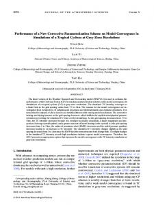
4. Results a. Climatological precipitation in the equatorial belt Previous observational studies indicate that the intraseasonal variance of convection is highly correlated with time-mean convective intensity (e.g., WK; Hendon et al. 1999). Therefore we first look at the climatological precipitation in the tropics, especially over the IndoPacific warm-pool region, where most of the convectively coupled equatorial waves have the largest variance (WK). Figure 1 shows the 8-yr time-mean precipitation for observations and the different model experiments. Most of the model experiments simulate excessive precipitation over the western Pacific Ocean warm pool, northwestern Pacific, South Pacific convergence zone (SPCZ), and eastern Pacific intertropical convergence zone (ITCZ), but insufficient precipitation over the Indian Ocean. The double-ITCZ problem is significant only in the Kuo-1 experiment, but not in the other experiments. Most of the IPCC AR4 AGCMs studied by Lin (2007) do not show a significant doubleITCZ problem. Increasing the strength of the moisture trigger generally suppresses precipitation over medium SST (SST ⬍ 28°C), especially over the eastern Pacific ITCZ, but does not change the precipitation much over the western Pacific warm pool or the Indian Ocean. To give a more quantitative comparison, Fig. 2 shows the annual-mean precipitation along the equatorial belt averaged between 15°N and 15°S. To focus on the large-scale features, we smoothed the data zonally to retain only zonal wavenumbers 0 through 6. Figure 2 demonstrates two points. First, all experiments except Kuo-1 simulate the basic features of observed precipitation reasonably, with the primary maximum over the Indo-Pacific warm-pool region, and a secondary local maximum over Central/South America. Kuo-1, on the other hand, produces overly high precipitation over the western Indian Ocean, the eastern Pacific, and the Atlantic Ocean, which is similar to many IPCC AR4 models (Lin et al. 2006). Within the warm-pool region, all experiments, except Kuo-1 and SAS-0, reproduce the local minimum of precipitation over the Maritime Continent, but there is a positive bias over the western Pacific and a negative bias over the eastern Indian Ocean. Outside the warm-pool region, all experiments
887
produce quite realistic magnitudes of precipitation over Central/South America. Second, although in some cases (Kuo-1 and SAS-0) adding/removing a moisture trigger causes significant change in climatological mean precipitation, in most of the cases it has little effect on the mean precipitation (e.g., Kuo-2 versus Kuo-3; SAS-1, SAS-2, and SAS-3; all MCA experiments), and thus any difference in their intraseasonal variability is likely due to the moisture trigger instead of a change in mean precipitation. In short, most of the model experiments simulate excessive precipitation over the western Pacific warm pool but insufficient precipitation over Indian Ocean. The double-ITCZ problem is significant only in the Kuo-1 experiment but not in other experiments. Changing the strength of the moisture trigger has little effect on the climatological mean precipitation in most of the cases, suggesting that in those cases any change in the intraseasonal variability is likely due to changes in the moisture trigger instead of changes in mean precipitation.
b. Total intraseasonal (2–128 day) variance and raw space–time spectra Figure 3 shows the total variance of the 2–128-day precipitation anomaly along the equator averaged between 15°N and 15°S. There are two important things to note concerning Fig. 3. First, despite the similar annual-mean precipitation over the Indo-Pacific warm pool in all experiments except Kuo-1 and SAS-0, the total intraseasonal variance displays a large scatter ranging from much smaller than observations to much larger than observations. There is a tendency for the models to have larger variance over the western Pacific than over the Indian Ocean, which is consistent with their tendency to have larger annual-mean precipitation over the western Pacific (Fig. 2). Among the three convection schemes, the MCA scheme tends to produces the largest variance, while the SAS scheme tends to produce the smallest variance and the Kuo scheme lies in between. Interestingly, the NO CONV experiment also produces one of the largest variances, which is similar to the MCA experiments and the Kuo-3 experiment with a nearly saturated RH trigger. Second, increasing the strength of the moisture trigger significantly enhances the total intraseasonal variance for the Kuo and SAS schemes. Note that Kuo-1 produces one of the smallest variances over the whole Indo-Pacific warm pool although it simulates the largest annual-mean precipitation over the Indian Ocean (Fig. 2). However, increasing the strength of the moisture trigger has little effect for the MCA scheme, which always produces the largest variances.
888
JOURNAL OF CLIMATE
VOLUME 21
FIG. 1. Annual-mean precipitation (shading) for observations (GPCP) and different model experiments. Contours indicate the observed SST used to force the model experiments. Contouring starts at 27°C with an interval of 1°C.
1 MARCH 2008
LIN ET AL.
889
FIG. 2. Annual-mean precipitation along the equatorial belt averaged between 15°N and 15°S for two observational datasets and 14 models. The data are smoothed zonally to keep only wavenumbers 0–6. The locations of continents within the equatorial belt are indicated by black bars under the abscissa.
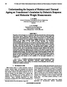
The symmetric space–time spectrum of the observational 1DD data is shown in Fig. 4a where, as in WK, the plotted contours are the logarithm of the power. The spectrum is very similar in shape to those obtained by WK, even though WK used OLR instead of the blend of precipitation estimates composing the 1DD
dataset. As in WK, the spectrum is very red in time and space, with most power at the largest spatial scales and lowest frequencies. Despite this redness, distinct spectral peaks and gaps are evident even in this raw spectrum. One obvious feature is the dominance of eastward over westward power at low wavenumbers and
FIG. 3. Variance of the 2–128-day precipitation anomaly along the equator averaged between 15°N and 15°S.
890
JOURNAL OF CLIMATE
VOLUME 21
FIG. 4. Space–time spectrum of 15°N–15°S symmetric component of precipitation. Frequency spectral width is 1/128 cpd.
frequencies, a signal corresponding to the MJO. Other peaks also correspond to known equatorial wave modes, and will be discussed further below. The remainder of Fig. 4 displays the corresponding
spectra from the various model experiments, using identical contour intervals and shading as in Fig. 4a (recall that these spectra are calculated for identical daily and 5° horizontal resolutions). Consistent with
1 MARCH 2008
LIN ET AL.
891
FIG. 4. (Continued)
their total intraseasonal variances (Fig. 3), the MCA scheme and NO CONV experiment produce the largest spectral powers in all frequencies and wavenumbers, while the SAS scheme tends to simulate the smallest power, and the Kuo scheme lies in between. For both the Kuo and the SAS schemes, increasing the strength of the moisture trigger significantly enhances the spectral power in all frequencies and wavenumbers. However, the effect is small for the MCA scheme. In addition, most of the experiments do not capture the same ratio of eastward to westward power at low wavenumbers and frequencies (i.e., the MJO region) as in observations (Fig. 3a). We will later show this ratio for the observations and models over specific spatial domains (cf. Fig. 9). The characteristics of the raw antisymmetric spectra, in terms of total power and redness, are generally similar to Fig. 4 and so will not be shown here. In summary, the MCA scheme and NO CONV experiment produce the largest total intraseasonal (2–128 day) variances of precipitation and the largest spectral powers in the space–time spectrum. Increasing the strength of the moisture trigger significantly enhances the total intraseasonal variance and spectral power for the Kuo and SAS schemes, but the effect for the MCA schemes is small. The NO CONV experiment always produces one of the largest variances and spectral powers, similar to the MCA experiments and the Kuo-3 experiment with a nearly saturated moisture trigger.
c. Dominant intraseasonal modes Figures 5 and 6 show the results of dividing the symmetric and antisymmetric raw spectra by the estimates of their background spectra. This normalization procedure removes a large portion of the systematic biases within the various models and observed datasets in Fig. 4, more clearly displaying the model disturbances with respect to their own climatological variance at each scale. Signals of the Kelvin, ER, and WIG waves are readily identified in the observational symmetric spectra (Fig. 5a), along with the MRG and EIG waves in the antisymmetric spectra (Fig. 6a). Dispersion curves of the shallow-water modes are also shown on all spectra, corresponding to equivalent depths of 12, 25, and 50 m. As in the OLR spectra of WK, all of the observed spectral peaks corresponding to shallow-water modes best match an equivalent depth of around 25 m in the observational rainfall data. All experiments display signals of convectively coupled equatorial waves, with Kelvin and MRG–EIG waves especially prominent. For each experiment, all modes scale similarly to a certain equivalent depth, which is indicative of similar physical processes linking the convection and large-scale disturbances within each experiment. Increasing the strength of the moisture trigger significantly slows down the phase speeds of Kelvin and MRG–EIG waves for both the Kuo and
892
JOURNAL OF CLIMATE
VOLUME 21
FIG. 5. Space–time spectrum of 15°N–15°S symmetric component of precipitation divided by the background spectrum. Superimposed are the dispersion curves of the odd meridional mode-numbered equatorial waves for equivalent depths of 12, 25, and 50 m. Frequency spectral width is 1/128 cpd.
SAS schemes, but the effect is small for the MCA scheme. The NO CONV experiment simulates prominent wave signals that have the slowest phase speeds among all experiments.
When a model displays signals of a certain wave mode in Figs. 5 and 6, it means that the variance of that wave mode stands out above the background spectra (i.e., a high signal-to-noise ratio), but the absolute value
1 MARCH 2008
LIN ET AL.
893
FIG. 5. (Continued)
of the variance of that wave mode may not be large. Therefore, it is of interest to look further at the absolute values of the variance of each wave mode. Figure 7 shows the variances of the (a) Kelvin, (b) ER, (c) MRG, (d) EIG, and (e) WIG modes along the equator averaged between 15°N and 15°S. There are three important conclusions that can be drawn from Fig. 7. First, increasing the strength of the moisture trigger significantly enhances the variance of all wave modes for both the Kuo and SAS schemes, but the effect is small and sometimes opposite for the MCA scheme. Second, the variance produced by the MCA scheme is always much larger than the observed variance. This is very encouraging since only 1 or 2 of the 14 IPCC AR4 models produce variances that are barely larger than observations. Third, the variance produced by the NO CONV experiment is always among the largest and is always much larger than the observed variance. In summary, all experiments display signals of convectively coupled equatorial waves, with Kelvin and MRG–EIG waves especially prominent. For both the Kuo and SAS schemes, increasing the strength of moisture trigger significantly enhances the variances and slows down the phase speeds of all wave modes. However, the effect is small for the MCA scheme, which always simulates prominent wave signals with variances much larger than observations. The NO CONV experiment also simulates prominent wave signals whose vari-
ances are among the largest and whose phase speeds are the slowest.
d. Variance of the MJO mode Now we focus on the variance of the MJO mode, that is, the daily variance in the MJO window of eastward wavenumbers 1–6 and periods of 30–70 days. Figure 8 shows the variance of the MJO anomaly along the equator averaged between 15°N and 15°S. Figure 8 demonstrates three points. First, many experiments with a moisture trigger produce a quite large MJO variance that is close to or larger than the observed value over the western Pacific. This is very encouraging, considering the fact that only 2 of the 14 IPCC AR4 GCMs analyzed by Lin et al. (2006) simulate an MJO variance that approaches the observed value. Second, although experiments with a moisture trigger generally produce larger MJO variances than those without a moisture trigger, increasing the strength of the moisture trigger does not increase the MJO variance monotonically, even for the Kuo and SAS schemes. For example, the Kuo-3 experiment produces smaller MJO variance than the Kuo-2 experiment over the western Pacific, as does SAS-3 versus SAS-2. This is in contrast with the monotonic increase in the variances of other wave modes for the Kuo and SAS schemes (Fig. 7). Therefore, even though increasing the strength of the moisture trigger
894
JOURNAL OF CLIMATE
VOLUME 21
FIG. 6. As in Fig. 5 but for the 15°N–15°S antisymmetric component of precipitation.
always enhances the variances of other convectively coupled equatorial waves, one has to choose a medium strength carefully in order to get a strong MJO variance. Third, the NO CONV experiment always produces one of the largest variances.
The inconsistent impact of moisture triggering on the model MJO mode is interesting. Most of the previous GCM studies showed that increasing the moisture trigger strength increases model MJO variance (e.g., Tokioka et al. 1988; Itoh 1989; Wang and Schlesinger 1999;
1 MARCH 2008
LIN ET AL.
895
FIG. 6. (Continued)
Zhang and Mu 2005), but a few studies found that increasing the moisture trigger strength actually decreases the strength of the MJO (Maloney and Hartmann 2001b). Our results suggest two possible reasons for the above discrepancy: 1) the strength of the moisture trigger used in different studies may lie in different regions of the parameter space, because our results suggest that the effect is not monotonic; and 2) some other schemes, such as the large-scale condensation scheme or shallow convection scheme, may significantly contribute to the wave-heating feedback and thus enhance or cancel the changes in deep convection scheme. Such effects are likely different in different models. In addition to the variance of the eastward MJO, another important index for evaluating the MJO simulation is the ratio between the variance of the eastward MJO and that of its westward counterpart, that is, the westward wavenumber 1 through 6, 30–70-day mode, which is important for the zonal propagation of tropical intraseasonal oscillations. Figure 9 shows the ratio between the eastward variance and the westward variance averaged over (a) an Indian Ocean box between 5°N– 5°S and 70°–100°E and (b) a western Pacific box between 5°N–5°S and 140°–170°E. In observations, the eastward MJO variance roughly triples the westward variance over both the Indian Ocean (Fig. 9a) and the western Pacific (Fig. 9b). Most of the experiments produce a smaller ratio. The MCA scheme often simulates
a ratio larger than the other two schemes. Increasing the strength of the moisture trigger generally increases the ratio for the Kuo and SAS schemes, but not for the MCA scheme. The NO CONV experiment always produces one of the largest ratios. The competition between the eastward MJO variance and its westward counterpart largely determines the zonal propagation characteristics of tropical intraseasonal oscillations. A useful method for evaluating the MJO simulation is to look at the propagation of 30–70-day filtered anomaly of the raw precipitation data, which includes all wavenumbers that dominate over other modes, as is the case in observations (e.g., Weickmann et al. 1985, 1997; Kiladis and Weickmann 1992; Lin and Mapes 2004). Because the tropical intraseasonal oscillation is dominated by zonally asymmetric, planetary-scale phenomena, the competition is mainly between the MJO and its westward counterpart—the westward wavenumber 1–6 component. Figure 10 shows the lag correlation of 30–70-day precipitation anomaly averaged between 5°N and 5°S with respect to itself at 0°, 85°E. The observational data show prominent eastward-propagating signals of the MJO, with a phase speed of about 7 m s⫺1. Consistent with the eastward/westward ratio in Fig. 9a, most of the experiments cannot reproduce the observed highly coherent eastward propagation. Nevertheless, increasing the strength of the moisture trigger improves the east-
896
JOURNAL OF CLIMATE
FIG. 7. Variances of (a) Kelvin, (b) ER, (c) MRG, (d) EIG, and (e) WIG modes along the equator averaged between 15°N and 15°S.
VOLUME 21
1 MARCH 2008
LIN ET AL.
897
FIG. 7. (Continued)
ward propagation for the Kuo and SAS schemes, although the phase speed is often too large, especially for the SAS scheme. The MCA scheme generally produces more coherent eastward propagation than the other two schemes. The NO CONV experiment simulates the best eastward propagation although the phase speed is a little too slow. The results are similar when using a western Pacific reference point (not shown). Next we apply more detailed scrutiny to the MJO precipitation variance by looking at the shape of the power spectrum. Figure 11a shows the raw spectra of the eastward wavenumber 1–6 component at 0°, 85°E. Because it is difficult to see the shape of the spectra for several models with very small variance, we also plotted
their normalized spectra (raw spectrum divided by its total variance) in Fig. 11b. Both of the two observational datasets show prominent spectral peaks between 30- and 70-day periods, with the power of 1DD lower than that of GPI. Most of the experiments do not show a pronounced spectral peak in the MJO frequency band, but show too red a spectrum; that is, the variance of the MJO band does not stand above but is simply embedded within a red-noise continuum. Increasing the strength of the moisture trigger enhances the prominence of the spectral peak for the Kuo scheme, but the effect is small for other schemes. Note the Kuo-1 experiment produces a spectrum quite similar to that of white noise, suggesting that the dominance of grid-scale
898
JOURNAL OF CLIMATE
VOLUME 21
FIG. 8. Variance of the MJO mode along the equator averaged between 15°N and 15°S.
convection, which is a well-known problem for wave– conditional instability of the second kind (CISK) modes (see review by Hayashi and Golder 1993). The MCA scheme always produces to some degree a spectral peak with periods between 30 and 45 days. The NO CONV experiment simulates the most realistic spectral peak. Results for 0°, 155°E (western Pacific) are similar (not shown). The redness of the model spectra shown in Fig. 11 brings to mind a “red noise” spectrum of a first-order linear Markov process (Gilman 1963; Jenkins and Watts 1968; Lin et al. 2006). For a first-order Markov process, the redness of the spectrum is determined by its lag-1 autocorrelation , which is hereinafter referred to as the persistence of the time series. Therefore we plot in Fig. 12 the autocorrelation function of precipitation at 0°, 85°E. Both observational datasets have a of about 0.7. The model experiments display a large scatter in the persistence of precipitation. The SAS scheme usually produces the largest persistence, while the MCA scheme usually produces the smallest persistence, and the Kuo scheme lies in between. The NO CONV experiment simulates one of the smallest persistences. Increasing the strength of moisture trigger does not monotonically change the persistence. Regarding the shape of the autocorrelation function, SAS-3 is closest to observation. Results for 0°, 155°E (western Pacific) are similar (not shown). To summarize, the MCA scheme generally produces larger MJO variance, more coherent eastward propagation of the MJO, and a more prominent MJO spectral peak than the Kuo and SAS schemes. Increasing the
strength of the moisture trigger does not monotonically enhance the MJO variance, but usually improves the eastward propagation of the MJO for the Kuo and SAS schemes. The NO CONV experiment produces one of the most realistic MJO signals in terms of variance, eastward propagation, and prominence of spectral peak.
5. Summary and discussion This study examines the impacts of convective parameterization and the moisture convective trigger on convectively coupled equatorial waves simulated by the SNU AGCM. Three different convection schemes are used, including the SAS scheme, the Kuo scheme, and the MCA scheme, and a moisture convective trigger with variable strength is added to each scheme. We also conduct a no convection experiment with the deep convection scheme turned off. Space–time spectral analysis is used to obtain the variance and phase speed of dominant convectively coupled equatorial waves, including the MJO, Kelvin, ER, MRG, EIG, and WIG waves. The results show that both convective parameterization and the moisture convective trigger have significant impacts on AGCM-simulated convectively coupled equatorial waves. The MCA scheme generally produces larger variances of convectively coupled equatorial waves including the MJO, more coherent eastward propagation of the MJO, and a more prominent MJO spectral peak than the Kuo and SAS schemes. Increasing the strength of the moisture trigger significantly enhances the variances and slows down the
1 MARCH 2008
LIN ET AL.
899
FIG. 9. Ratio between the MJO variance and the variance of its westward counterpart (westward wavenumber 1–6, 30–70-day mode). The variances are averaged over (a) an Indian Ocean box between 5°N–5°S and 70°–100°E, and (b) a western Pacific box between 5°N–5°S and 140°–170°E.
phase speeds of all wave modes except the MJO. This usually improves the eastward propagation of the MJO for the Kuo and SAS schemes, but the effect for MCA scheme is small.
An interesting result of this study is that the no convection experiment always produces one of the best signals of convectively coupled equatorial waves and the MJO. In the early generations of GCMs, without a
900
JOURNAL OF CLIMATE
VOLUME 21
FIG. 10. Lag correlation of the 30–70-day precipitation anomaly averaged along the equator between 5°N and 5°S with respect to itself at 0°, 85°E. The three thick lines correspond to phase speeds of 3, 7, and 15 m s⫺1, respectively.
deep convection scheme, the model often became unstable. But now with the improvement of dynamical cores, GCMs can work properly without a deep convection scheme. Even when the deep convection
scheme is on, the large-scale condensation scheme is still in action and contributes to the total precipitation and heating. How does the large-scale condensation affect the experiments with the deep convection scheme
1 MARCH 2008
901
LIN ET AL.
FIG. 10. (Continued)
on? Figure 13 shows the ratio between time-mean large-scale precipitation and time-mean total precipitation averaged between 15°N and 15°S. For the no convection experiment, as expected, all precipitation comes from large-scale precipitation and the ratio is always 1. For the MCA scheme, about half of the precipitation comes from large-scale precipitation, and the ratio does not change much for different strengths of moisture trigger. For the Kuo and SAS schemes, when the moisture trigger becomes stronger and stronger, the ratio becomes larger. Therefore, the better simulation of waves by the MCA scheme and the Kuo and SAS schemes with stronger moisture triggers are associated with greater contributions of large-scale condensation in those experiments. The large-scale condensation scheme, by design, is very sensitive to environmental moisture. This further supports the importance of moisture control on deep convection for simulating the convectively coupled equatorial waves; although the effect may not be through the deep convection scheme, it is represented in the model by the large-scale condensation scheme. A similar sensitivity of convectively coupled equatorial waves to the fraction of convective versus largescale condensation has been identified in an idealized moist GCM in Frierson (2007a), with slower and more intense waves occurring with more large-scale condensation. In the Frierson (2007a) study, the changes in
phase speed and intensity are interpreted in terms of the gross moist stability (GMS) of the atmosphere (Neelin and Held 1987), which is reduced with more large-scale condensation. We next calculate this quantity for these simulations, using the following definition for the GMS, ⌬m: · V2 ⫽
冕 冕
ps
pm
⌬m ⫽
·V
dp , g
ps
0
m · V
and
共3兲
dp 共 · V2兲⫺1, g
共4兲
where overbars denote time means, ps is the surface pressure, V is the horizontal velocity, m ⫽ cpT ⫹ gz ⫹ Lq is the moist static energy (with cp the specific heat at constant pressure for dry air, T the temperature, g the gravitational acceleration, z the geopotential, L the latent heat of vaporization, and q the specific humidity), and pm is a midtropospheric level. The midtropospheric level pm is chosen so that the quantity · V2 is maximized for each column. In first baroclinic mode models of the tropical atmosphere with moisture (e.g., Neelin and Zeng 2000; Frierson et al. 2004), the GMS or some analogous quantity determines the speed of convectively coupled equatorial waves by setting the effective static stability in moist regions. In these theories the wave speeds scale with the square root of the GMS. The GMS (divided by cp to have units of kelvins) is plotted
902
JOURNAL OF CLIMATE
VOLUME 21
FIG. 11. Spectra of the eastward wavenumber 1–6 component of equatorial precipitation (5°N–5°S) at 0°, 85°E for two observational datasets and 14 models: (a) raw spectrum; (b) normalized spectrum. Frequency spectral width 1/100 cpd.
for two regions in Fig. 14: in Fig. 14a is the GMS averaged over a region in the equatorial Indian Ocean, between 5°N and 5°S latitude and 65° and 93°E longitude, and in Fig. 14b is the GMS averaged over a region in the equatorial west Pacific Ocean, between 5°N and 5°S latitude and 160°E and 172°W longitude. These regions are chosen as the regions with generally maximum variance of precipitation within each ocean basin for the simulations. It is clear that as in the idealized GCM
simulations of Frierson (2007a), the GMS is decreased significantly for the simulations with slower phase speeds. For instance, the Kuo-1 simulation has largest GMS of any simulation, while the Kuo-2 and Kuo-3 simulations are significantly reduced when compared with these. The SAS simulations experience an approximately 50% reduction in GMS in each region as the moisture trigger strength is increased. The MCA simulations, the NO CONV simulation, and the SAS-3
1 MARCH 2008
LIN ET AL.
903
FIG. 12. Autocorrelation of precipitation at 0°, 85°E.
simulation have roughly equally small GMS values. However, there is some spatial character to the GMS, as values tend to be larger in the Indian Ocean than in the west Pacific. In Frierson (2007b), an explanation is given for the reduction of the gross moist stability in terms of the typical depths of convection. Reducing the depths of convection may also enhance the second and higher vertical modes, and many theoretical studies have shown that interactions between different vertical
modes tend to slow down the phase speed of the moist waves (e.g., Mapes 2000; Majda and Shefter 2001; Majda et al. 2004; Haertel and Kiladis 2004; Khouider and Majda 2006, 2007). In a companion paper, we examine the determination and relevance of different definitions of the gross moist stability to wave speeds, as well as composites of vertical structures and other features of the waves. How does the moisture control of deep convection
904
JOURNAL OF CLIMATE
VOLUME 21
FIG. 13. The ratio between time-mean large-scale precipitation and time-mean total precipitation averaged between 15°N and 15°S.
enhance the convectively coupled equatorial waves? The moisture control can affect the waves by changing either the time-mean moisture field or the moisture anomaly associated with the waves. We plot in Fig. 15 the time-mean total precipitable water (PW) along the equator. Except for the Kuo-1 experiment, there is no significant difference among different experiments for each scheme. For example, Kuo-2 and Kuo-3 experiments have nearly identical time-mean PW, but Kuo-3 has much stronger convectively coupled equatorial waves. All SAS experiments have similar mean PW, but increasing the strength of the moisture trigger significantly improves the waves. Therefore, the effect of the
moisture trigger is not through changing the time-mean PW, but through changing the moisture anomaly associated with the waves. Our results provide a contrast to the findings of Maloney and Hartmann (2001b), who found that the time-mean PW strongly affects the simulated MJO variance in their GCM with higher timemean PW leading to larger MJO variance. Why, then, does the moisture anomaly affect the variances of the waves? It is widely accepted that waveheating feedback plays a central role in amplifying and maintaining the convectively coupled equatorial waves. The column-integrated diabatic heating anomaly has six major components: the free-troposphere moisture
FIG. 14. Gross moist stability for the different experiments for (a) an Indian Ocean box between 65° and 93°E longitude and (b) a western Pacific box between 160°E and 172°W longitude, both between 5°N and 5°S latitude.
1 MARCH 2008
LIN ET AL.
905
FIG. 15. Annual-mean total precipitable water along the equator averaged between 5°N and 5°S.
convergence, the boundary layer moisture convergence, the surface heat flux anomaly (latent plus sensible) due to wind variation, the local moisture tendency, the radiative heating, and the surface heat flux anomaly due to SST variation. These six components have been emphasized by wave-CISK (e.g., Lau and Peng 1987; Chang and Lim 1988; Hendon 1988; Dunkerton and Crum 1991), frictional wave–CISK (e.g., Wang and Rui 1990; Salby et al. 1994), windinduced surface heat exchange (WISHE; e.g., Emanuel 1987; Neelin et al. 1987), charge–discharge (e.g., Bladé and Hartmann 1993; Hayashi and Golder 1997; Khouider and Majda 2006, 2007), cloud–radiation interaction (e.g., Raymond 2001; Lee et al. 2001; Bony and Emanuel 2005; Zurovac-Jevtic´ et al. 2006; Lin et al. 2007), and air–sea coupling (e.g., Flatau et al. 1997; Wang and Xie 1998; Waliser et al. 1999) theories, respectively. These mechanisms also interact with one another, with the vertical heating structure (e.g., Mapes 2000; Majda and Shefter 2001; Haertel and Kiladis 2004; Khouider and Majda 2006), and with nonlinear effects of subscale perturbations (e.g., Majda and Klein 2003; Moncrieff 2004; Biello and Majda 2005, 2006; Majda 2007). The moisture anomaly is involved directly in at least four of the above feedback mechanisms: the wave-CISK, frictional wave–CISK, charge–discharge, and air–sea coupling mechanisms. A stronger moisture trigger makes the moisture higher during deep convection, which is associated with low-level convergence,
and therefore increases the moisture convergence per unit mass convergence and enhances the waves through the wave-CISK and frictional wave–CISK feedbacks. A stronger moisture trigger also prolongs the time for moisture to build up before deep convection can occur, and therefore increases the periods of the waves through the charge–discharge mechanism. On the contrary, a stronger moisture trigger may lead to higher boundary layer moisture, which tends to suppress surface latent heat flux and thus suppress the waves through the air–sea coupling mechanism, but this suppressing effect on latent heat flux is likely smaller than the enhancing effect on boundary layer moisture convergence. Changing the strength of moisture trigger in deep convection scheme may also indirectly affect the cloudradiative fluxes and cloud–radiation feedback. In a companion paper, Lin et al. (2007) found that enhanced cloud-radiative heating tends to suppress many convectively coupled equatorial waves. To examine this possibility, Fig. 16 shows the linear regression of daily ⫺OLR against precipitation, which is a good measure of how much cloud-radiative heating enhances the column-integrated latent heating (Lin and Mapes 2004). The effect of the moisture trigger is different for different schemes. For the MCA scheme, increasing the strength of the moisture trigger does not change the cloud-radiative heating much. For the Kuo scheme, increasing the strength of the moisture trigger enhances
906
JOURNAL OF CLIMATE
VOLUME 21
FIG. 16. Linear regression of daily ⫺OLR against precipitation along the equator averaged between 5°N and 5°S. The same units are used for both variables so that the regression coefficient is unitless.
the cloud-radiative heating from Kuo-1 to Kuo-2 (which by itself tends to suppress many waves), but not from Kuo-2 to Kuo-3. Thus the monotonic enhancement of variances from Kuo-1 to Kuo-3 in many waves is not due to cloud–radiation feedback. On the other hand, for the SAS scheme, increasing the strength of the moisture trigger reduces the cloud-radiative heating, which contributes to the enhancement of variance in many waves. Acknowledgments. This study benefited greatly from discussions with Wanqiu Wang, the insightful reviews of Prof. Sandrine Bony, and three anonymous reviewers. J. L. Lin was supported by the NOAA CPO/CVP Program, NOAA CPO/CDEP Program, and NASA MAP Program. I.-S. Kang and D. Kim have been supported by the Korea Meteorological Administration Research and Development Program under Grant CATER_2007-4206 and BK21 program. D. M. W. Frierson is supported by the NOAA Climate and Global Change Postdoctoral Fellowship, administered by the University Corporation for Atmospheric Research. REFERENCES Arakawa, A., and W. H. Schubert, 1974: Interaction of a cumulus cloud ensemble with the large-scale environment, part I. J. Atmos. Sci., 31, 674–701. Bergman, J. W., H. H. Hendon, and K. M. Weickmann, 2001: Intraseasonal air–sea interactions at the onset of El Niño. J. Climate, 14, 1702–1719.
Bessafi, M., and M. C. Wheeler, 2006: Modulation of south Indian Ocean tropical cyclones by the Madden–Julian oscillation and convectively coupled equatorial waves. Mon. Wea. Rev., 134, 638–656. Biello, J. A., and A. J. Majda, 2005: A new multiscale model for the Madden–Julian oscillation. J. Atmos. Sci., 62, 1694–1721. ——, and ——, 2006: Modulating synoptic scale convective activity and boundary layer dissipation in the IPESD models of the Madden–Julian oscillation. Dyn. Atmos. Oceans, 42, 152– 215. Bladé, I., and D. L. Hartmann, 1993: Tropical intraseasonal oscillations in a simple nonlinear model. J. Atmos. Sci., 50, 2922– 2939. Bonan, G. B., 1996: A land surface model (LSM version 1.0) for ecological, hydrological, and atmospheric studies: Technical description and user’s guide. NCAR Tech. Note NCAR/TN417⫹STR, National Center for Atmospheric Research, Boulder, CO, 150 pp. Bony, S., and K. A. Emanuel, 2005: On the role of moist processes in tropical intraseasonal variability: Cloud–radiation and moisture–convection feedbacks. J. Atmos. Sci., 62, 2770– 2789. Chang, C.-P., and H. Lim, 1988: Kelvin wave-CISK: A possible mechanism for the 30–50 day oscillations. J. Atmos. Sci., 45, 1709–1720. Dunkerton, T. J., and F. X. Crum, 1991: Scale selection and propagation of wave-CISK with conditional heating. J. Meteor. Soc. Japan, 69, 449–458. Emanuel, K. A., 1987: An air–sea interaction model of intraseasonal oscillations in the Tropics. J. Atmos. Sci., 44, 2324–2340. Flatau, M., P. J. Flatau, P. Phoebus, and P. P. Niiler, 1997: The feedback between equatorial convection and local radiative and evaporative processes: The implications for intraseasonal oscillations. J. Atmos. Sci., 54, 2373–2386.
1 MARCH 2008
LIN ET AL.
Frierson, D. M. W., 2007a: Convectively coupled Kelvin waves in an idealized moist general circulation model. J. Atmos. Sci., 64, 2076–2090. ——, 2007b: The dynamics of idealized convection schemes and their effect on the zonally averaged tropical circulation. J. Atmos. Sci., 64, 1959–1976. ——, A. J. Majda, and O. M. Pauluis, 2004: Large scale dynamics of precipitation fronts in the tropical atmosphere: A novel relaxation limit. Comm. Math. Sci., 2, 591–626. Gilman, D. L., F. J. Fuglister, and J. M. Mitchell Jr., 1963: On the power spectrum of “red noise.” J. Atmos. Sci., 20, 182–184. Haertel, P. T., and G. N. Kiladis, 2004: Dynamics of 2-day equatorial waves. J. Atmos. Sci., 61, 2707–2721. Hayashi, Y., and D. G. Golder, 1986: Tropical intraseasonal oscillations appearing in a GFDL general circulation model and FGGE data. Part I: Phase propagation. J. Atmos. Sci., 43, 3058–3067. ——, and A. Sumi, 1986: The 30-40 day oscillations simulated in an “aqua planet” model. J. Meteor. Soc. Japan, 64, 451–467. ——, and D. G. Golder, 1988: Tropical intraseasonal oscillations appearing in a GFDL general circulation model and FGGE data. Part II: Structure. J. Atmos. Sci., 45, 3017–3033. ——, and ——, 1993: Tropical 40–50- and 25–30-day oscillations appearing in realistic and idealized GFDL climate models and the ECMWF dataset. J. Atmos. Sci., 50, 464–494. ——, and ——, 1997: United mechanisms for the generation of low- and high-frequency tropical waves. Part I: Control experiments with moist convective adjustment. J. Atmos. Sci., 54, 1262–1276. Hendon, H. H., 1988: A simple model of the 40–50 day oscillation. J. Atmos. Sci., 45, 569–584. ——, C. Zhang, and J. D. Glick, 1999: Interannual variation of the Madden–Julian oscillation during austral summer. J. Climate, 12, 2538–2550. Holtslag, A. A. M., and B. A. Boville, 1993: Local versus nonlocal boundary-layer diffusion in a global climate model. J. Climate, 6, 1825–1842. Huffman, G. J., R. F. Adler, M. M. Morrissey, D. T. Bolvin, S. Curtis, R. Joyce, B. McGavock, and J. Susskind, 2001: Global precipitation at one-degree daily resolution from multisatellite observations. J. Hydrometeor., 2, 36–50. Itoh, H., 1989: The mechanism for the scale selection of tropical intraseasonal oscillations. Part I: Selection of wavenumber 1 and the three-scale structure. J. Atmos. Sci., 46, 1779–1798. Janowiak, J. E., and P. A. Arkin, 1991: Rainfall variations in the tropics during 1986–1989, as estimated from observations of cloud-top temperature. J. Geophys. Res., 96 (Suppl.), 3359– 3373. Jenkins, G. M., and D. G. Watts, 1968: Spectral Analysis and Its Applications. Holden-Day, 525 pp. Kemball-Cook, S. R., and B. C. Weare, 2001: The onset of convection in the Madden–Julian oscillation. J. Climate, 14, 780– 793. Kessler, W. S., M. J. McPhaden, and K. M. Weickmann, 1995: Forcing of intraseasonal Kelvin waves in the equatorial Pacific. J. Geophys. Res., 100, 10 613–10 632. Khouider, B., and A. J. Majda, 2006: A simple multicloud parameterization for convectively coupled tropical waves. Part I: Linear analysis. J. Atmos. Sci., 63, 1308–1323. ——, and ——, 2007: A simple multicloud parameterization for convectively coupled tropical waves. Part II: Nonlinear simulations. J. Atmos. Sci., 64, 381–400.
907
Kiladis, G. N., and K. M. Weickmann, 1992: Circulation anomalies associated with tropical convection during northern winter. Mon. Wea. Rev., 120, 1900–1923. ——, K. H. Straub, and P. T. Haertel, 2005: Zonal and vertical structure of the Madden–Julian oscillation. J. Atmos. Sci., 62, 2790–2809. Kuo, H. L., 1974: Further studies of the parameterization of the influence of cumulus convection of large-scale flow. J. Atmos. Sci., 31, 1232–1240. Lau, K.-M., and L. Peng, 1987: Origin of low-frequency (intraseasonal) oscillations in the tropical atmosphere. Part I: Basic theory. J. Atmos. Sci., 44, 950–972. Lau, N.-C., I. M. Held, and J. D. Neelin, 1988: The Madden– Julian oscillation in an idealized general circulation model. J. Atmos. Sci., 45, 3810–3832. Lee, M.-I., I.-S. Kang, J.-K. Kim, and B. E. Mapes, 2001: Influence of cloud-radiation interaction on simulating tropical intraseasonal oscillation with an atmospheric general circulation model. J. Geophys. Res., 106, 14 219–14 234. ——, ——, and B. E. Mapes, 2003: Impacts of cumulus convection parameterization on aqua-planet AGCM simulations of tropical intraseasonal variability. J. Meteor. Soc. Japan, 81, 963–992. Le Trent, H., and Z.-X. Li, 1991: Sensitivity of an atmospheric general circulation model to prescribed SST changes: Feedback effects associated with the simulation of cloud optical properties. Climate Dyn., 5, 175–187. Liebmann, B., H. H. Hendon, and J. D. Glick, 1994: The relationship between tropical cyclones of the western Pacific and Indian Oceans and the Madden–Julian oscillation. J. Meteor. Soc. Japan, 72, 401–412. Lin, J.-L., 2007: The double-ITCZ problem in IPCC AR4 coupled GCMs: Ocean–atmosphere feedback analysis. J. Climate, 20, 4497–4525. ——, and B. E. Mapes, 2004: Radiation budget of the tropical intraseasonal oscillation. J. Atmos. Sci., 61, 2050–2062. ——, and Coauthors, 2006: Tropical intraseasonal variability in 14 IPCC AR4 climate models. Part I: Convective signals. J. Climate, 19, 2665–2690. ——, D. Kim, M.-I. Lee, and I.-S. Kang, 2007: Effects of cloudradiative heating on AGCM simulations of convectively coupled equatorial waves. J. Geophys. Res. 112, D24107, doi:10.1029/2006JD008291. Madden, R. A., and P. R. Julian, 1971: Detection of a 40–50 day oscillation in the zonal wind in the tropical Pacific. J. Atmos. Sci., 28, 702–708. Majda, A. J., 2007: New multiscale models and self-similarity in tropical convection. J. Atmos. Sci., 64, 1393–1404. ——, and M. G. Shefter, 2001: Models for stratiform instability and convectively coupled waves. J. Atmos. Sci., 58, 1567– 1584. ——, and R. Klein, 2003: Systematic multiscale models for the tropics. J. Atmos. Sci., 60, 393–408. ——, B. Khouider, G. N. Kiladis, K. H. Straub, and M. G. Shefter, 2004: A model for convectively coupled tropical waves: Nonlinearity, rotation, and comparison with observations. J. Atmos. Sci., 61, 2188–2205. Maloney, E. D., and D. L. Hartmann, 1998: Frictional moisture convergence in a composite life cycle of the Madden–Julian oscillation. J. Climate, 11, 2387–2403.
908
JOURNAL OF CLIMATE
——, and ——, 2000: Modulation of eastern North Pacific hurricanes by the Madden–Julian oscillation. J. Climate, 13, 1451– 1460. ——, and ——, 2001a: The Madden–Julian oscillation, barotropic dynamics, and North Pacific tropical cyclone formation. Part I: Observations. J. Atmos. Sci., 58, 2545–2558. ——, and ——, 2001b: The sensitivity of intraseasonal variability in the NCAR CCM3 to changes in convective parameterization. J. Climate, 14, 2015–2034. Manabe, S., J. Smagorinsky, and R. F. Strickler, 1965: Simulated climatology of a general circulation model with a hydrologic cycle. Mon. Wea. Rev., 93, 769–798. Mapes, B. E., 2000: Convective inhibition, subgrid-scale triggering energy, and stratiform instability in a toy tropical wave model. J. Atmos. Sci., 57, 1515–1535. Matsuno, T., 1966: Quasi-geostrophic motions in the equatorial area. J. Meteor. Soc. Japan, 44, 25–43. Moncrieff, M. W., 2004: Analytic representation of the large-scale organization of tropical convection. J. Atmos. Sci., 61, 1521– 1538. Moorthi, S., and M. J. Suarez, 1992: Relaxed Arakawa–Schubert: A parameterization of moist convection for general circulation models. Mon. Wea. Rev., 120, 978–1002. Myers, D. S., and D. E. Waliser, 2003: Three-dimensional water vapor and cloud variations associated with the Madden– Julian oscillation during Northern Hemisphere winter. J. Climate, 16, 929–950. Nakajima, T., M. Tsukamoto, Y. Tsushima, and A. Numaguti, 1995: Modelling of the radiative processes in an AGCM. Climate System Dynamics and Modelling, Vol. I-3, T. Matsuno, Ed., Center for Climate System Research, 104–123. Neelin, J. D., and I. M. Held, 1987: Modeling tropical convergence based on the moist static energy budget. Mon. Wea. Rev., 115, 3–12. ——, and N. Zeng, 2000: A quasi-equilibrium tropical circulation model—Formulation. J. Atmos. Sci., 57, 1741–1766. ——, I. M. Held, and K. H. Cook, 1987: Evaporation–wind feedback and low-frequency variability in the tropical atmosphere. J. Atmos. Sci., 44, 2341–2348. Numaguti, A., M. Takahashi, T. Nakajima, and A. Sumi, 1995: Development of an atmospheric general circulation model. Climate System Dynamics and Modelling, Vol. I-3, T. Matsuno, Ed., Center for Climate System Research, 1–27. Raymond, D. J., 2001: A new model of the Madden–Julian oscillation. J. Atmos. Sci., 58, 2807–2819. Roundy, P. E., and G. N. Kiladis, 2006: Observed relationships between oceanic Kelvin waves and atmospheric forcing. J. Climate, 19, 5253–5272. Salby, M. L., and R. R. Garcia, 1987: Transient response to localized episodic heating in the Tropics. Part I: Excitation and short-time near-field behavior. J. Atmos. Sci., 44, 458–498. ——, ——, and H. H. Hendon, 1994: Planetary-scale circulations in the presence of climatological and wave-induced heating. J. Atmos. Sci., 51, 2344–2367. Seo, K.-H., and K.-Y. Kim, 2003: Propagation and initiation mechanisms of the Madden–Julian oscillation. J. Geophys. Res., 108, 4384, doi:10.1029/2002JD002876. Slingo, J. M., K. R. Sperber, J.-J. Morcrette, and G. L. Potter, 1992: Analysis of the temporal behavior of convection in the
VOLUME 21
tropics of the European Centre for Medium-Range Weather Forecasts model. J. Geophys. Res., 97, 18 119–18 135. ——, and Coauthors, 1996: Intraseasonal oscillations in 15 atmospheric general circulation models: Results from an AMIP diagnostic subproject. Climate Dyn., 12, 325–357. Sperber, K. R., 2003: Propagation and the vertical structure of the Madden–Julian oscillation. Mon. Wea. Rev., 131, 3018–3037. Takayabu, Y. N., 1994: Large-scale cloud disturbances associated with equatorial waves. Part I: Spectral features of the cloud disturbances. J. Meteor. Soc. Japan, 72, 433–449. ——, T. Iguchi, M. Kachi, A. Shibata, and H. Kanzawa, 1999: Abrupt termination of the 1997–98 El Niño in response to a Madden–Julian oscillation. Nature, 402, 279–282. Tian, B., D. E. Waliser, E. J. Fetzer, B. H. Lambrigtsen, Y. L. Yung, and B. Wang, 2006: Vertical moist thermodynamic structure and spatial-temporal evolution of the MJO in AIRS observations. J. Atmos. Sci., 63, 2462–2485. Tiedtke, M., 1983: The sensitivity of the time-mean large-scale flow to cumulus convection in the ECMWF model. Proc. Workshop on Convection in Large-Scale Numerical Models, Reading, United Kingdom, European Centre for MediumRange Weather Forecasts, 297–316. Tokioka, T., K. Yamazaki, A. Kitoh, and T. Ose, 1988: The equatorial 30-60-day oscillation and the Arakawa-Schubert penetrative cumulus parameterization. J. Meteor. Soc. Japan, 66, 883–901. Waliser, D. E., K. M. Lau, and J.-H. Kim, 1999: The influence of coupled sea surface temperatures on the Madden–Julian oscillation: A model perturbation experiment. J. Atmos. Sci., 56, 333–358. ——, S. Schubert, A. Kumar, K. Weickmann, and R. Dole, 2003: Proceedings from a workshop on “Modeling, Simulation and Forecasting of Subseasonal Variability.” NASA/CP 2003104606, Vol. 25, 62 pp. Wang, B., and H. Rui, 1990: Dynamics of the coupled moist Kelvin–Rossby wave on an equatorial -plane. J. Atmos. Sci., 47, 397–413. ——, and X. Xie, 1998: Coupled modes of the warm pool climate system. Part I: The role of air–sea interaction in maintaining Madden–Julian oscillation. J. Climate, 11, 2116–2135. Wang, W., and M. E. Schlesinger, 1999: The dependence on convection parameterization of the tropical intraseasonal oscillation simulated by the UIUC 11-layer atmospheric GCM. J. Climate, 12, 1423–1457. Weickmann, K. M., G. R. Lussky, and J. E. Kutzbach, 1985: Intraseasonal (30–60 day) fluctuations of outgoing longwave radiation and 250 mb streamfunction during northern winter. Mon. Wea. Rev., 113, 941–961. ——, G. N. Kiladis, and P. D. Sardeshmukh, 1997: The dynamics of intraseasonal atmospheric angular momentum oscillations. J. Atmos. Sci., 54, 1445–1461. Wheeler, M. C., and G. N. Kiladis, 1999: Convectively coupled equatorial waves: Analysis of clouds and temperature in the wavenumber–frequency domain. J. Atmos. Sci., 56, 374–399. ——, and J. L. McBride, 2005: Australian-Indonesian monsoon. Intraseasonal Variability in the Atmosphere-Ocean Climate System, W. K. M. Lau and D. E. Waliser, Eds., SpringerPraxis, 125–173. ——, G. N. Kiladis, and P. J. Webster, 2000: Large-scale dynamical fields associated with convectively coupled equatorial waves. J. Atmos. Sci., 57, 613–640.
1 MARCH 2008
LIN ET AL.
Yang, G.-Y., B. Hoskins, and J. Slingo, 2003: Convectively coupled equatorial waves: A new methodology for identifying wave structures in observational data. J. Atmos. Sci., 60, 1637–1654. Yasunari, T., 1979: Cloudiness fluctuations associated with the Northern Hemisphere summer monsoon. J. Meteor. Soc. Japan, 57, 227–242. Yuter, S. E., and R. A. Houze Jr., 2000: The 1997 Pan American Climate Studies Tropical Eastern Pacific Process Study.
909
Part I: ITCZ region. Bull. Amer. Meteor. Soc., 81, 451– 481. Zhang, G. J., and M. Mu, 2005: Simulation of the Madden–Julian oscillation in the NCAR CCM3 using a revised Zhang– McFarlane convection parameterization scheme. J. Climate, 18, 4046–4064. Zurovac-Jevtic´ , D., S. Bony, and K. Emanuel, 2006: On the role of clouds and moisture in tropical waves: A two-dimensional model study. J. Atmos. Sci., 63, 2140–2155.