The Inventory-Routing Problem with Transshipment - CIRRELT

___________________________ The Inventory-Routing Problem with Transshipment Leandro Callegari Coelho Jean-François Cordeau Gilbert Laporte

March 2011

CIRRELT-2011-21

Bureaux de Montréal :

Bureaux de Québec :

Université de Montréal C.P. 6128, succ. Centre-ville Montréal (Québec) Canada H3C 3J7 Téléphone : 514 343-7575 Télécopie : 514 343-7121

Université Laval 2325, de la Terrasse, bureau 2642 Québec (Québec) Canada G1V G1V0A6 0A6 Téléphone : 418 656-2073 Télécopie : 418 656-2624

www.cirrelt.ca

The Inventory-Routing Problem with Transshipment Leandro Callegari Coelho1,2,*, Jean-François Cordeau1,2, Gilbert Laporte1,3 1 2

3

Interuniversity Research Centre on Enterprise Networks, Logistics and Transportation (CIRRELT) Department of Logistics and Operations Management, HEC Montréal, 3000 Côte-SainteCatherine, Montréal, Canada H3T 2A7 Department of Management Sciences, HEC Montréal, 3000 Côte-Sainte-Catherine, Montréal, Canada H3T 2A7

Abstract. This paper introduces the Inventory-Routing Problem with Transshipment (IRPT). This problem arises when vehicle routing and inventory decisions must be made simultaneously, which is typically the case in vendor-managed inventory systems. Heuristics and exact algorithms have already been proposed for the Inventory-Routing Problem (IRP), but these algorithms ignore the possibility of performing transshipments between customers so as to further reduce the overall cost. We present a formulation that allows transshipments, either from the supplier to customers or between customers. We also propose an adaptive large neighborhood search heuristic to solve the problem. This heuristic manipulates vehicle routes while the remaining problem of determining delivery quantities and transshipment moves is solved through a network flow algorithm. Our approach can solve four different variants of the problem: the IRP and the IRPT, under maximum level and order-up-to level policies. We perform an extensive assessment of the performance of our heuristic. Keywords. Inventory-routing problem, transshipment, ALNS, heuristic. Acknowledgements. This work was partly supported by the Natural Sciences and Engineering Council of Canada (NSERC) under grants 227837-09 and 39682-10. This support is gratefully acknowledged. The authors thank Glaydston M. Ribeiro for his help with computations at an early stage of this work, as well as Andrew Goldberg and Boris Cherkassky for making their implementation of the scaling push-relabel minimum-cost flow algorithm available.

Results and views expressed in this publication are the sole responsibility of the authors and do not necessarily reflect those of CIRRELT. Les résultats et opinions contenus dans cette publication ne reflètent pas nécessairement la position du CIRRELT et n'engagent pas sa responsabilité.

_____________________________ * Corresponding author: [email protected] Dépôt légal – Bibliothèque et Archives nationales du Québec Bibliothèque et Archives Canada, 2011 © Copyright Callegari Coelho, Cordeau, Laporte and CIRRELT, 2011

The Inventory-Routing Problem with Transshipment

1

Introduction

Logistics is now widely recognized as a value adding center in organizations through product availability, consistency of deliveries, accuracy in inventory and demand management, and ease of placing orders. Vendor-managed inventory (VMI) is one of the most up-to-date examples of value added through logistics. This practice constitutes a streamlined approach to inventory management in which the supplier makes replenishment decisions based on specific inventory and supply chain policies. Vendor-managed inventory is a win-win situation: suppliers save on distribution and production costs since they can combine and coordinate demands and shipments for different customers, and buyers gain by not allocating resources to controlling and managing inventories. The supplier then has to make three simultaneous decisions: 1) when to serve a given customer, 2) how much to deliver, and 3) how to combine customers into routes. Regarding the size of deliveries, one of two policies is typically applied: the order-up-to (OU) policy or the maximum level (ML) policy. Under the OU policy the quantity delivered to a customer is that to fill its inventory capacity; under the ML policy the supplier can decide how much to deliver to a customer, as long as its holding capacity is respected [20]. In addition to these features, this paper introduces the concept of transshipment within inventory-routing. Under this policy, goods may be shipped to a customer who experiences a shortage, either directly from the supplier or from another customer. This occurs, for example, between stores belonging to a same chain [21, 22] which can ship merchandise to one another when the need occurs. From a practical point of view, the use of a transshipment option contributes to lead-time and cost reductions. The drawback of VMI is that it requires the solution of a very difficult mathematical problem, called the Inventory-Routing Problem (IRP), itself a combination of two well-studied problems: inventory management and vehicle routing. According to Andersson et al. [1] “no commercially available systems provide decision support for combined inventory management and routing”. Scientific research on the IRP is relatively recent compared to that on other optimization problems, such as the Vehicle Routing Problem (VRP). Speranza and Ukovich [30] note the existence of distinct extensive literature reviews on transportation and on inventory management problems, but relatively few studies exploit their integration. This is still true to this day. A quick search on the ABI/INFORM Global database shows over 580 scholarly publications on the VRP, but less than 70 on the IRP. Recent reviews on the IRP found fewer than a hundred papers addressing the combined VRP-inventory management problem [1, 10]. Several variants of the IRP have arisen since this problem was first introduced by Bell et al. [5]. These include the IRP with a single customer [6, 11, 31], the IRP with multiple customers [2, 5, 8, 16], the stochastic IRP [16, 17, 18], the IRP with direct deliveries [12, 13, 15, 16, 19], the multi-item IRP [4, 26, 29, 30], and the IRP with heterogeneous fleet [8, 9, 24]. There are so many ways of modeling and solving IRPs that different authors rarely define the problem in

CIRRELT-2011-21

1


exactly the same way. In addition, real-life problems combining vehicle routing and inventory management concerns are often dynamic or stochastic. We next describe three important algorithms for the IRP which we will use as benchmarks for our own algorithm. Bertazzi et al. [7] study the case with multiple retailers, dynamic deterministic demand rates and the OU policy. They compute the quantity to be delivered to each customer for each combination of time instants and insert it in the cheapest position. The solution is then iteratively improved by selecting customer pairs, removing them from the current solution and reinserting them. Any improving move is implemented. The first exact algorithm for the IRP is that of Archetti et al. [2]. It handles the single-vehicle case without backlogging, under the OU inventory policy. This algorithm is based on a classical branch-and-cut scheme in which the subtour elimination constraints are initially relaxed. Branching is performed in priority on the assignment of customers to delivery periods, and then on routing variables. The instances solved in this paper have become standard benchmarks. Recently, Archetti et al. [3] have developed a hybrid heuristic combining tabu search and integer programming for the same problem. Starting from a feasible solution, the algorithm explores the neighbourhood of the current solution and performs occasional jumps to new regions of the search space. Infeasible solutions are temporarily accepted, namely due to a stockout at the supplier or exceeded vehicle capacity. Reverting to the main theme of this paper, the concept of transshipment appears in the work of [21, 22, 23] but has not yet been formally integrated within the context of inventory-routing. Its inclusion adds an extra layer of complexity to an already difficult problem. For this reason, we believe it is unrealistic to contemplate the use of an exact algorithm for the IRPT. We have therefore developed an adaptive large neighbourhood search (ALNS) heuristic for it. This type of algorithm was initially put forward by [27] in the context of the VRP and extends a concept initially proposed by Shaw [28]. The algorithm we propose is designed to handle the specific features of the IRPT. It is flexible and can easily handle the OU and ML replenishment policies. The main scientific contributions of this paper are the introduction of a transshipment option within the context of inventory-routing and the development of a powerful and flexible ALNS heuristic to solve four variants of the problem: the IRPT with transshipment (IRPT) and the IRP without transshipment (IRP), under an OU or an ML replenishment policy. These four variants will be referred to as IRPT-OU, IRPT-ML, IRP-OU and IRP-ML. The remainder of the paper is organized as follows. In Section 2 we introduce and describe the IRP. Section 3 presents a mixed-integer linear programming formulation for the four variants of the problem considered in the paper, and for a restriction in which routing is fixed. In Section 4 we present our ALNS algorithm, followed by computational results, in Section 5, and by our conclusions in Section 6.

2

CIRRELT-2011-21


2

Problem description

We now formally introduce the IRPT. The problem is defined on a graph G = (V, A) where V = {0, ..., n} is the vertex set and A is the arc set. Vertex 0 represents the supplier and the vertices of V 0 = V \{0} represent customers. Both the supplier and customers incur unit inventory holding costs hi per period (i ∈ V), and each customer has an inventory holding capacity Ci . The length of the planning horizon is p and, at each time period t ∈ T = {1, ..., p} the quantity of product made available at the supplier is rt . We assume the supplier has enough inventory to meet all the demand during the planning horizon and that inventories are not allowed to be negative, i.e., the supplier can only ship what he holds in stock with no backlogging option. At the beginning of the planning horizon the decision maker knows the current inventory level of the supplier and of the customers (I00 and Ii0 ), and receives the information on the demand dti of each customer i for each time period t. A single vehicle of capacity Q is available. This vehicle is able to perform one route at the beginning of each time period to deliver products from the supplier to a subset of customers. A routing cost cij is associated with arc (i, j) ∈ A. Transshipments can be made later in the time period. A transshipment can start from the depot or from any customer in a subset R ⊆ V 0 , i.e., these customers can dispatch goods to other customers as needed. Transshipments can occur when it is profitable to ship goods from the depot to a customer on a special request basis, or from customer i ∈ R to customer j ∈ V 0 . This can be done by subcontracting to a carrier who will pickup goods either at the supplier or from any transshipment point. These outsourced deliveries are only made by direct shipping and the unit cost associated with transshipping products from i to j is bij . It is possible that both the supplier’s vehicle and the subcontractor visit the same customer within the same time period: the supplier’s vehicle first delivers to the customer according to the OU or to the ML policy, and the subcontractor may later deliver to that customer according to the ML policy. We also assume that all orders and deliveries can be performed during the same time period, which means that lead times are negligible. The objective of the problem is to minimize the total cost while meeting the demand for each customer. The replenishment plan is subject to the following constraints: • inventories at each customer can never exceed the maximal available inventory capacity; • inventories are not allowed to be negative, i.e., all demand must be met by previous inventory plus deliveries performed during the time period considered; • if the supplier’s vehicle visits a customer in a time period, an OU or an ML replenishment policy applies;

CIRRELT-2011-21

3


• the supplier’s vehicle can perform at most one route per time period, starting and ending at the supplier; • the vehicle capacity cannot be exceeded. The solution to the problem should determine: • which customers to serve in each time period using the supplier’s vehicle; • which route to use in each time period; • how much to transship from every i ∈ R ∪ {0} to every j ∈ V 0 in each time period.

3

Mathematical models

In addition to the notation already introduced, we define an artificial period p + 1 and the set T 0 = T ∪ {p + 1}. The model works with the following binary variables: xtij is equal to 1 if and only if customer j immediately follows customer i on the route of the supplier’s vehicle in period t. Let the quantity of product delivered from the supplier to each customer i at each time period t be t yit and let also wij be the amount of product delivered directly from i ∈ R ∪ {0} to customer j ∈ V 0 at period t using the outsourced carrier.

3.1

Model for IRPT-OU

In the IRPT, the total cost to be minimized is the sum of inventory holding costs at the supplier and at the customers, of routing costs for the supplier’s vehicle and of transshipment costs: min

X t∈T

0

h0 I0t +

X X i∈V 0

t∈T

0

hi Iit +

XXX

X

cij xtij +

i∈V j∈V t∈T

i∈R∪{0}

XX j∈V 0

t bij wij . (1)

t∈T

The constraints are as follows: 3.1.1 Inventory definition at the supplier The inventory level at the supplier in period t is defined at the beginning of the period and is given by its previous inventory level (period t − 1), plus the quantity rt−1 made available in period t − 1, minus the total quantity shipped to the customers using the supplier’s vehicle in period t − 1, minus the total quantity transshipped to the customers in period t − 1: I0t = I0t−1 + rt−1 −

X i∈V 0

yit−1 −

X

t−1 w0i

t ∈ T 0,

(2)

i∈V 0

0 where r0 = yi0 = w0i = 0, i ∈ V 0 .

4

CIRRELT-2011-21


3.1.2 Stockout constraints at the supplier These constraints impose that the supplier’s inventory cannot be less than the total amount of product delivered in period t: I0t ≥

X

t (yit + w0i ) t∈T.

(3)

i∈V 0

3.1.3 Inventory definition at the customers Likewise, the inventory level at each retailer in period t is given by its previous inventory level in period t−1, plus the quantity yit−1 delivered by the supplier’s vehicle in period t − 1, plus the total quantity transshipped in period t − 1, minus the total quantity transshipped to other customers in period t − 1, minus its demand in period t − 1, that is:

Iit = Iit−1 + yit−1 +

X

t−1 wji −

X

t−1 wij − dt−1 i

i ∈ V0

t ∈ T 0 . (4)

j∈V 0

j∈R∪{0}

3.1.4 Stockout constraints at the customers These constraints guarantee that for each customer i ∈ V 0 the inventory level Iit remains non-negative at all time: Iit ≥ 0 i ∈ V

t ∈ T 0.

(5)

3.1.5 Maximal inventory level at the customers These constraints guarantee that for each customer i ∈ V 0 the inventory level Iit remains below the maximum level Ci at all time: Iit ≤ Ci

i∈V

t ∈ T 0.

(6)

3.1.6 Quantities delivered These sets of constraints ensure that the quantity delivered by the supplier’s vehicle to each customer i ∈ V 0 in each period t ∈ T will fill the customer’s inventory capacity if the customer is served, and will be zero otherwise: yit ≥ Ci

X

xtij − Iit

i ∈ V0

t∈T;

(7)

j∈V 0

yit ≤ Ci − Iit i ∈ V 0 t ∈ T ; X yit ≤ Ci xtij i ∈ V 0 t ∈ T . j∈V

CIRRELT-2011-21

5

(8) (9)


If customer i is not visited in period t, then constraints (9) mean that the quantity delivered to it will be zero (while constraints (7) and (8) are still respected). If, otherwise, customer i is visited in period t, constraints (9) limit the quantity delivered to the customer’s inventory holding capacity, and this bound is tightened by constraints (8), making it impossible to deliver more than what would exceed this capacity. Constraints (7) model the OU replenishment policy, ensuring that the quantity delivered will be exactly the bound provided by constraints (8). 3.1.7 Vehicle capacity These constraints guarantee that the vehicle’s capacity is not exceeded: X

yit ≤ Q

t∈T.

(10)

i∈V 0

3.1.8 Routing constraints These constraints guarantee that a feasible route is determined to visit all customers served in period t: a) Flow conservation constraints: these constraints impose that the number of arcs entering and leaving a vertex should be the same: X

xtij =

X

i∈V

xtji

j∈V

t∈T.

(11)

i∈V

b) A single vehicle is available: X

xti0 ≤ 1 t ∈ T .

(12)

i∈V

c) Subtour elimination constraints: vit − vjt + Qxtij ≤ Q − yjt yit ≤ vit ≤ Q

i ∈ V0 i ∈ V0

j ∈ V0

t∈T;

t∈T.

(13)

(14)

3.1.9 Integrality and nonnegativity constraints t vit , yit , wji ≥ 0 i ∈ V0

xtij

∈ {0, 1}

j ∈ R ∪ {0} t ∈ T ;

i, j ∈ V, i 6= j

6

t∈T.

(15) (16)

CIRRELT-2011-21


3.2

Adaptations to IRPT-ML, IRP-OU and IRP-ML

This model can be modified to enforce the ML replenishment policy by dropping t constraints (7). Similarly, to forbid transshipments one only has to set all wij variables equal to zero. Thus all four versions of the IRPT can be modeled through the same formulation.

3.3

Model for the IRPT with fixed routes

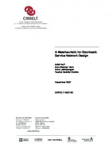
If one fixes routing variables xtij , the remaining problem reduces to a network t variables. The flow conservation flow problem defined by the Iit , yit and wij equations are given by (2) and (4). The lower and upper bounds on the flows are defined by (3) and (5)−(9). Vehicle capacity constraints (10) still define an upper bound on the quantity delivered by the vehicle, even though the customers to be visited are fixed. Constraints (11)−(13) are not relevant in the flow models because their variables are fixed. Figure 1 depicts the network flow model for a small network with two customers and two time periods. The supplier and the customers are represented by vertices replicated for each time period, plus one extra set of vertices for initial inventories, and one extra set for the decisions made at the last time period. The supplier and each customer carry their inventories between successive time periods. The corresponding solid arcs in the figure have unit inventory holding costs, and the flows on these arcs are bounded above by the customer’s inventory capacity (infinite for the supplier). At each period t the supplier receives rt units of the product and customer i has a demand equal to dti . The vehicle is represented by one vertex at each period, receiving an arc from the supplier at the same period with a flow up to Q units and no cost associated to it, and is then connected to each customer receiving a delivery at that period, a decision made by the ALNS heuristic, also with no cost. These arcs are dashed in Figure 1 at period two, supposing that the ALNS has decided to make a visit to customer 2 only. We have added dotted arcs representing transshipment options from the supplier and from every customer to every other customer. For the sake of clarity, Figure 1 only shows these arcs for period 1, but they are actually present in all periods. This allows the network flow solution to serve a given customer through a transshipment if a later routing delivery would violate vehicle capacity, or if any inventory constraint is not satisfied by the routing decisions. The OU policy is enforced by fixing the flow on the arcs linking customers in different successive time periods: once customer i is visited in period t, the arc connecting it to itself at the next period has a flow equal to Ui −dti . The network flow algorithm only computes the quantities delivered from all transshipment arcs, as the quantities delivered by the supplier are fixed by the OU policy. When the ML replenishment policy is in place, no extra action is needed.

CIRRELT-2011-21

7


Initial conditions

Period p+1

Periods r

1

r

2

1

Supplier

0

0

d1

1

Customers 2

2

0

Dummy sink

2

d1

1

I1

1

1

d2

I0

0

1

w

1

2

I0

2

I1

1

2

d2

1

I2

2

2

I2

2

y

Supplier’s vehicle

Inventory conservation arcs Vehicle routes arcs (fixed by the ALNS) Transshipment arcs

Figure 1: Network flow problem for two customers and two time periods.

4

Adaptive large neighborhood search heuristic

We now describe our ALNS heuristic. The main framework is made up of four components. 1. Large neighborhood: At each iteration, a number of customers are removed from their current route and are eventually reinserted. This fixes the decisions regarding routing, and the problem is passed to a network flow solver to optimize all remaining decisions simultaneously (minimize total costs taking into account inventory holding costs, transshipments and delivery quantities), as described in Section 3.3. 2. Adaptive search engine: The choice of which movement to perform is governed by a roulette-wheel mechanism in which each movement is assigned a weight depending on its past performance. Let ωi be a measure of how well movement i has performed in the past; then given h moves h P with weights ωi , movement j will be selected with probability ωj / ωi . i=1

3. Adaptive weight adjustment: The search is divided into segments of ϕ iterations each, and weights are computed by taking into account the performance of the movements during the last segment. In the first

8

CIRRELT-2011-21


segment all movements have the same weight. At each iteration, scores are updated as follows: if a movement finds a new best solution, its score is increased by σ1 ; if it finds a solution better than the incumbent, its score is increased by σ2 ; if the solution is not better but is still accepted, the score is increased by σ3 . Obviously σ1 > σ2 > σ3 . After ϕ iterations, the weights are updated considering the scores obtained in the last segment and scores are reset to zero. To do so, let πi and oij be, respectively, the score of the movement i and the number of times movement i has been used in the last segment j. Then,

ωi,j+1

( ωij = (1 − η)ωij + ηπi /oij

if oij = 0 if oij = 6 0,

(17)

where η ∈ [0, 1] is called the reaction factor, controling how quickly the weight adjustment reacts to changes in the movement performance. 4. Acceptance and stopping criteria: We use the same acceptance criteria as in simulated annealing: given a solution s, a neighbor solution 0 s’ is accepted if z(s0 ) < z(s), and with probability e−(z(s )−z(s))/τ otherwise, where z(s) is the solution cost defined by (1) and τ > 0 is the current temperature. The temperature starts at τstart and is decreased by a cooling rate factor φ at each iteration, where 0 < φ < 1. To avoid long computations for large and difficult instances, we limit the running time to one hour and also to a maximum number of iterations, as described in Section 4.3.

4.1

Initial solution

The initial solution is generated by randomly selecting 75% of the customers and randomly assigning them to some periods of the planning horizon. Their insertion in the routes follows the cheapest insertion rule. Our computational experiments have shown that the initial solution does not have a significant impact on the overall solution cost or running time.

4.2

List of movements

Unlike related problems like the VRP, where every removal is accompanied by an insertion, one may decide to remove a vertex from some periods and not reinsert it back. This partial solution will still be feasible when transshipments are made. Moreover, in the IRPT family, it is feasible and sometimes optimal not to create any route because transshipments can always be made. This observation has motivated us not to use the traditional destroy and repair framework of Shaw [28] and Pisinger and Ropke [25] in which each destroy move is always followed by a repair move, but to keep the option of making only a removal or only an insertion.

CIRRELT-2011-21

9


As in Pisinger and Ropke [25] we artificially increase the score of complex movements because they are much more time consuming than the others. This reduces the probability of selecting them. In what follows, ρ is an integer randomly drawn from the interval [1, n] using a semi-triangular distribution with a negative slope. 4.2.1 Randomly remove ρ This movement randomly selects one period and removes one customer from it. It is repeated ρ times. This movement is useful for refining the solution, since it does not change it much when ρ is small (which happens frequently), but still yields a major transformation when ρ is large. 4.2.2 Randomly insert ρ This movement randomly inserts ρ customers into the current solution. Specifically, it selects one random customer and one random period, and inserts the customer into the route of that period if the customer is not yet routed. This movement is repeated ρ times. 4.2.3 Remove worst ρ This movement removes the customer that will save the most when removed, considering the total routing, inventory and transshipment cost. It is repeated ρ times. 4.2.4 Insert best ρ This movement is analogous to the previous one. It is repeated ρ times by computing the cheapest insertion with respect to total costs. 4.2.5 Shaw removal Following the ideas developed by Ropke and Pisinger [27] and by Shaw [28] this movement removes customers that are relatively close to each other. Specifically, this heuristic randomly selects one period from the planning horizon and one customer served in this period, computes the distance distmin to the closest customer also being served by the same route, and removes all customers within 2distmin units from the selected route. 4.2.6 Shaw insertions This movement is similar to the Shaw removal in the sense that it selects similar customers to be inserted together. It selects one period and one customer not served in that period. The heuristic then computes distmin and all customers within a 2distmin distance are inserted in the same period, always following the cheapest insertion rule. 4.2.7 Remove ρ customers This movement is repeated ρ times by selecting one customer and removing it from all routes where it appears. The motivation for this movement is to allow these customers to be assigned to different sets of periods.

10

CIRRELT-2011-21


4.2.8 Insert ρ customers This heuristic is repeated ρ times by selecting one customer and assigning it to several randomly selected periods if the customer is not yet present in those periods. The motivation is to diversify the search towards unexplored areas of the search space, allowing customers to be served in different periods from the ones currently selected. 4.2.9 Empty one period This movement randomly selects one period and removes all customers from it. The motivation is to allow different periods to have opened routes. 4.2.10 Swap routes This movement randomly selects two periods and swaps their routes. 4.2.11 Randomly move ρ This movement selects one period and one customer being served in this period, removes it and serves it in a different randomly selected period. It is repeated ρ times. 4.2.12 Multiple Interchanges This movement is used only in IRP-OU and IRPT-OU since we observed that for these variants the remaining movements were not sufficient: due to the OU policy, the insertion of a customer in the incumbent solution has a great impact e.g. on inventory costs and on the load of the vehicle. This heuristic is an adaptation of the ideas developed by Bertazzi et al. [7] and differs from the original algorithm described in Section 1 by three key elements: 1) it does not iterate while there is an improvement, but the number of iterations is equal to n/2; 2) it does not restart afresh at each call, but it is initiated from the incumbent solution; 3) it applies some improvement procedures to take transshipments into account as they were not present in the original algorithm: if a customer has a lower inventory cost than that of the supplier, products are transshipped to that customer if the tradeoff is positive, while respecting its inventory holding capacity; transshipments are combined to an early period if this yields savings, and routes from the last periods are replaced by transshipments, since one could save on inventory holding costs if the OU policy did not have to be enforced.

4.3

Solution procedure

We now describe our ALNS pseudocode and the parameters that govern the algorithm. We have tested different combinations for the parameters during a tuning phase. The starting temperature τstart is set to 30,000 and the cooling rate φ is 0.9994, which yields roughly 25,000 iterations, our desired number of repetitions. The stopping criterion is satisfied when the temperature reaches

CIRRELT-2011-21

11


0.01, when 25,000 iterations have been performed, or when 3,600 seconds have elapsed. In our implementation, the segment length ϕ was set to 200 iterations and the reaction factor η was set to 0.7, that is, new weights will be composed by 70% of the performance on the last segment and 30% by the last weight value. Scores are updated with σ1 = 10, σ2 = 5 and σ3 = 2. Algorithm 1 shows the pseudocode for our ALNS.

4.4

ALNS applied to the IRPT-OU

In this section we briefly describe how our ALNS is implemented for the IRPTOU. Once the ALNS has fixed the routing variables, the remaining problem is modeled as a network flow problem and solved by means of a specialized minimum cost network flow algorithm, as described in Section 3. It is easy to see that if all transshipments are set to zero, the problem reduces to IRP-OU which yields an upper bound on the IRPT-OU optimum.

4.5

ALNS applied to the IRPT-ML

This version of the problem is similar to the IRPT-OU except that the arcs connecting customers between successive time periods do not force the flow to respect the OU policy. The network flow algorithm determines the quantities delivered by the vehicle and from all transshipment arcs. Once again, if all transshipments are zero, the problem reduces to an IRP-ML which yields an upper bound on the IRPT-ML optimum.

4.6

ALNS applied to the IRP-OU

We have applied our algorithm to the IRP-OU without any structural change. To avoid passing an infeasible problem to the network flow algorithm (for instance when vehicle capacity would be exceeded or when a stockout would occur at a customer due to it not being served as often as required), we have kept all transshipment arcs from the supplier and from every customer to every other customer, with large artificial costs; this means that feasible solutions can always be reached, but at very high cost if transshipments are used. These costs act as penalties in the objective function when the vehicle capacity is exceeded or when the master level heuristic does not add all customers to the current solution. The remaining problem is then similar to the IRPT-OU: decisions regarding routings are fixed by the ALNS algorithm and modeled as a network flow problem with one vertex representing the vehicle for each period, and arcs leaving the vehicle vertex and arriving at each selected customer. The vehicle vertex receives an arc from the supplier with up to Q units of flow. The OU policy is modeled by fixing the flow on the arcs connecting customers in successive time periods: once customer i is visited in period t, the arc linking to it in the next period has a flow equal to Ui − dti .

12

CIRRELT-2011-21


Algorithm 1 ALNS 1: Initialize: set weights of all removal and insertion heuristics equal to 1 and all scores equal to 0. 2: s ← initial solution. 3: sbest ← s. 4: τ ← τstart . 5: while τ > 0.01 and time < 3,600 and iterations < 25,000 do 6: s0 ← s. 7: Select a movement using the roulette-wheel mechanism based on the weights of the current segment. 8: Apply the movement to s0 and update the number of times it is used. 9: Fix routing decisions, solve the remaining problem taking into account inventory holding costs, inventory policy and transshipment cost. 10: if f (s0 ) < f (s) then 11: s ← s0 ; 12: if f (s) < f (sbest ) then 13: sbest ← s; 14: update the score for the heuristic used with σ1 ; 15: else 16: update the score for the heuristic used with σ2 ; 17: end if 18: else 19: if s0 is accepted by the simulated annealing criterion then 20: s ← s0 ; 21: update the score for the heuristic used with σ3 . 22: end if 23: end if 24: if the end of the segment is reached then 25: update the weights of all heuristics and reset their scores. 26: end if 27: Adjust the cooling factor in order to decrease the temperature to 0.01 by the end of the running time if 25,000 iterations will not be met. 28: if time > 1,200 and iterations < 25,000/3 then 29: c ← (0.01/τ )1/(2·iterations) ; 30: end if 31: if time > 2,700 and iterations < 25,000/2 then 32: c ← (0.01/τ )1/(iterations/2) ; 33: end if 34: τ ← φτ ; 35: end while 36: Every 200 iterations perform an intra-route 2-opt to improve the sequence of customers. 37: return sbest ;

CIRRELT-2011-21

13


4.7

ALNS applied to the IRP-ML

Modeling the IRP-ML as a network flow problem is similar to the IRP-OU, except that arcs connecting the customers in successive time periods have a minimum flow equal to 0. The vehicle vertex is fed from the supplier with up to Q units and the minimum-cost network flow algorithm decides on how much to deliver to each of the customers selected from the master level heuristic. Dummy arcs are again inserted to penalize unvisited customers and solutions that would require exceeded vehicle capacity. It is easy to see that the IRP-OU yields an upper bound on the IRP-ML optimum as we just relaxed one constraint of the former problem.

5

Computational results

Our algorithm was coded in C++ using Microsoft Visual Studio 2008. We used the scaling push-relabel algorithm for the minimum-cost flow problem developed by Goldberg [14] to solve the second level problem. All computations were executed on an Intel Core2Duo 2.4GHz and 4 GB RAM laptop PC unless otherwise noted. To evaluate the performance of our heuristic, we have used the instances of the IRP generated and solved to optimality by Archetti et al. [2]. These were adapted to account for transshipments as described in Section 2. For the cases with transshipment, there are no previous reported solutions since we are introducing the problem in this paper. We have compared our algorithm against a truncated execution of CPLEX with a time limit of 3,600s. In Tables 1 to 4 we report both the upper bound (UB) and lower bound (LB) obtained by CPLEX and our solutions for the IRPT-OU. Results for the IRPTML are reported in Tables 5 to 8. Our algorithm was able to find better solutions than CPLEX for most of the instances on all sets. Our solutions were on average 8.2% better than those obtained by CPLEX for the IRPT-OU. They were better on all four sets of instances and up to 15.5% better for the set with six time periods and low inventory holding costs. For the IRPT-ML, our solutions were also better on all sets of instances. They were on average 12.4% better than those obtained by CPLEX, and up to 21.6% better for the same set.

14

CIRRELT-2011-21


Table 1: Results for the IRPT-OU - low inventory cost (hi ∈ [0.01, 0.05]), p = 3 and transshipment cost bij = 0.01cij Instance abs1n05 abs2n05 abs3n05 abs4n05 abs5n05 abs1n10 abs2n10 abs3n10 abs4n10 abs5n10 abs1n15 abs2n15 abs3n15 abs4n15 abs5n15 abs1n20 abs2n20 abs3n20 abs4n20 abs5n20 abs1n25 abs2n25 abs3n25 abs4n25 abs5n25 abs1n30 abs2n30 abs3n30 abs4n30 abs5n30 abs1n35 abs2n35 abs3n35 abs4n35 abs5n35 abs1n40 abs2n40 abs3n40 abs4n40 abs5n40 abs1n45 abs2n45 abs3n45 abs4n45 abs5n45 abs1n50 abs2n50 abs3n50 abs4n50 abs5n50 averages

LB 403.42 435.55 1477.9 811.6 598.5 1555.97 1791.97 1414.45 1589 1729.03 1868.08 1799.19 2083.5 1768.37 1735.96 2111.2 2107.63 2368.33 2482.39 2301.67 2419.52 2196.78 2438.52 2644.68 2406.76 2791.91 2731.55 3200.53 2822.03 2518.92 2674.14 2750.55 3156.77 2526.47 2755.31 2847.05 2677.75 2858.37 2814.08 2943.5 3131.23 2891.89 3332.12 3124.94 2972.11 3102.19 3479.7 3349.33 3751 3200.86

Truncated CPLEX UB gap (%) 403.42 0.00 435.55 0.00 1477.9 0.00 811.6 0.00 598.5 0.00 1555.97 0.00 1792.14 0.01 1414.45 0.00 1589 0.00 1729.03 0.00 1868.2 0.01 1799.32 0.01 2083.5 0.00 1768.54 0.01 1736.13 0.01 2111.4 0.01 2107.85 0.01 2368.56 0.01 2482.64 0.01 2627.72 14.17 2491.58 2.98 2416.78 10.01 3055.47 25.30 2644.94 0.01 2941.66 22.22 3594.42 28.74 3352.79 22.74 3268 2.11 2822.31 0.01 2578.61 2.37 3410.86 27.55 4050.83 47.27 4912 55.60 3412.11 35.05 5798.41 110.44 4397.81 54.47 4426.09 65.29 4218.64 47.59 3185.24 13.19 6427.93 118.38 4397.81 40.45 4793.16 65.74 4442.81 33.33 4689.98 50.08 4379.24 47.34 8279.76 166.90 5857.72 68.34 5862.01 75.02 4780.49 27.45 7679.78 139.93 28.40

time (s) 0.05 0.02 0.02 0.02 0.2 2.68 4.72 1.34 1.53 1.18 8.01 20.51 5.72 55.85 7.82 303.11 270.84 201.48 951.5 1060.99* 3600 3600 1174.95* 237.34 822.73* 1219.03* 1599.76* 3600 167.22 3600 1636.51* 1161.77* 1465.55* 1563.09* 870.64* 1077.4* 1303.44* 1051.46* 3600 1769.30* 1077.40* 1844.69* 1489.38* 1220.59* 1923.16* 1646.65* 1348.19* 1391.51* 1555.00* 2112.26*

*: aborted prematurely with out-of-memory status

CIRRELT-2011-21

15

z 403.42 435.55 1477.9 811.6 598.5 1555.97 1792.14 1418.35 1592.08 1729.03 1869.92 1821.5 2083.5 1777.68 1770.93 2181.68 2156.4 2446.22 2853.81 2574.09 2723.09 2416.78 2946.49 2809.97 2727.04 3934.12 3686.85 3492.05 3001.25 2593.21 3413.06 3426.5 4071.77 3041.2 3660.77 3590.06 4057.71 3952.64 3486.88 3890.74 4194.48 4127.35 4046.94 4187.81 3837.87 4627.87 4596.44 4814.94 4267.96 4598.16

ALNS gap (%) 0.00 0.00 0.00 0.00 0.00 0.00 0.01 0.28 0.19 0.00 0.10 1.24 0.00 0.53 2.01 3.34 2.31 3.29 14.96 11.84 12.55 10.01 20.83 6.25 13.31 40.91 34.97 9.11 6.35 2.95 27.63 24.58 28.99 20.37 32.86 26.10 51.53 38.28 23.91 32.18 33.96 42.72 21.45 34.01 29.13 49.18 32.09 43.76 13.78 43.65 16.95

time (s) 6.29 6.44 6.86 5.61 7.64 25.98 25.65 24.46 43.81 27.91 93.41 59.81 67.32 115.58 75.1 226.12 115.58 135.33 264.2 175.22 468.76 288.1 287.87 566.61 334.21 688.76 450.11 473.99 985 581.1 862.51 820.61 744.67 1070.35 977.45 1749.51 1444.81 1280.53 1561.28 1849.93 2062.53 2166.34 2441.85 2357 2723.47 2659.18 2775.06 2635.58 3154.88 3265.63


Table 2: Results for the IRPT-OU - high inventory cost (hi ∈ [0.1, 0.5]), p = 3 and transshipment cost bij = 0.01cij Instance abs1n05 abs2n05 abs3n05 abs4n05 abs5n05 abs1n10 abs2n10 abs3n10 abs4n10 abs5n10 abs1n15 abs2n15 abs3n15 abs4n15 abs5n15 abs1n20 abs2n20 abs3n20 abs4n20 abs5n20 abs1n25 abs2n25 abs3n25 abs4n25 abs5n25 abs1n30 abs2n30 abs3n30 abs4n30 abs5n30 abs1n35 abs2n35 abs3n35 abs4n35 abs5n35 abs1n40 abs2n40 abs3n40 abs4n40 abs5n40 abs1n45 abs2n45 abs3n45 abs4n45 abs5n45 abs1n50 abs2n50 abs3n50 abs4n50 abs5n50 averages

LB 1264.68 1215.1 2700.63 1374.54 1766.95 4346.14 4064.6 3560.61 3741.2 4506.63 5313.39 5111.27 5893.92 4574.78 4451.86 6656.3 6687.38 7116.31 6302.75 7329.12 7637.86 8056.15 8795.79 8037.04 9585.88 11363.33 10242.24 11607 9137.24 9312.08 10897.68 9704.67 13117.51 9584.75 10173.45 12495.91 10012.48 12533.76 10553.25 12346.84 13405.93 12291.24 14185.29 12640.85 12824.24 13627.44 13945.74 14159.08 15821.14 14538.68

Truncated CPLEX UB gap (%) 1264.68 0.00 1215.1 0.00 2700.63 0.00 1374.54 0.00 1766.95 0.00 4346.37 0.01 4064.91 0.01 3560.61 0.00 3741.2 0.00 4506.63 0.00 5313.91 0.01 5111.63 0.01 5894.51 0.01 4575.23 0.01 4452.29 0.01 6656.97 0.01 6688.05 0.01 7117.7 0.02 6303.39 0.01 7619.91 3.97 7857.37 2.87 8144.19 1.09 9226.77 4.90 8037.85 0.01 9790.28 2.13 12253.99 7.84 11015.1 7.55 11987.65 3.28 9138 0.01 9430.34 1.27 11762.54 7.94 10525.81 8.46 14346.29 9.37 10342.5 7.91 11067.73 8.79 14600.99 16.85 11795.18 17.80 13579.84 8.35 12026.21 13.96 13585.76 10.03 17873.64 33.33 17670.52 43.77 17545.85 23.69 14802.9 17.10 14450.5 12.68 17599.87 29.15 17171.48 23.13 16601.35 17.25 16625.97 5.09 18631.79 28.15 7.56

time (s) 0.08 0.03 0.03 0.02 0.19 2.78 4.82 1.3 1.56 1.55 9.96 20.94 5.31 40 27 149.73 501.72 86.45 1125.22 1559.46* 3600 3600 1040.78* 654.55 1608.23* 1173.78* 876.63* 2048.46* 90.56 2623.48* 3600 1043.51* 1392.86* 1052.61* 1022.67* 1405.78* 1294.77* 1699.26* 1335.46* 1403.73* 1309.94* 1409.93* 1118.45* 1678.70* 1619.63* 2459.93* 1353.16* 1820.37* 2651.43* 1763.14*

z 1264.68 1215.1 2700.63 1374.54 1766.95 4346.37 4064.91 3560.61 3741.2 4506.63 5330.77 5185.14 5894.51 4718.36 4452.29 6697.4 6757.64 7193.38 6382.71 7605.69 7989.53 8217.01 9224.65 8122.5 10216.5 12803.6 10727.4 12196.7 9151.62 9456.55 11692.6 10309.4 13801.1 10061.1 10971 13394.2 11338.7 13332.6 11389.7 13360.6 14139.3 13475.8 14864.1 13479.3 13648.2 15087.5 14649.8 15180.1 16540.5 16342.4

ALNS gap (%) 0.00 0.00 0.00 0.00 0.00 0.01 0.01 0.00 0.00 0.00 0.33 1.45 0.01 3.14 0.01 0.62 1.05 1.08 1.27 3.77 4.60 2.00 4.88 1.06 6.58 12.67 4.74 5.08 0.16 1.55 7.29 6.23 5.21 4.97 7.84 7.19 13.25 6.37 7.93 8.21 5.47 9.64 4.79 6.63 6.43 10.71 5.05 7.21 4.55 12.41 4.07

time (s) 6.74 6.54 13 6.87 7.16 25.4 25.37 47.2 27.27 25.39 60.26 63.63 113.57 71.98 63.76 123.86 135.16 219.96 126.62 150.49 256.01 298.13 615.94 304.34 276.73 495.66 520.6 652.61 460.87 477.87 740.74 955.9 1048.32 1050.93 854.51 1210.87 1614.09 1361.27 1395.97 2306.02 1729.56 2167.07 2106.52 3047.63 2169.29 3134.47 360 2920.84 3600 3600


16

CIRRELT-2011-21


Table 3: Results for the IRPT-OU - low inventory cost (hi ∈ [0.01, 0.05]), p = 6 and transshipment cost bij = 0.01cij Instance abs1n05 abs2n05 abs3n05 abs4n05 abs5n05 abs1n10 abs2n10 abs3n10 abs4n10 abs5n10 abs1n15 abs2n15 abs3n15 abs4n15 abs5n15 abs1n20 abs2n20 abs3n20 abs4n20 abs5n20 abs1n25 abs2n25 abs3n25 abs4n25 abs5n25 abs1n30 abs2n30 abs3n30 abs4n30 abs5n30 averages

LB 2571.02 1904.36 4002.84 2502.57 1828.09 3305.14 3135.07 3471.98 3608.24 4103.32 3996.79 3686.22 4625.68 3264.35 3830.77 3998.34 4155.49 4345.56 4816.81 4668.53 3837.32 4413.36 5042.47 5205.72 4707.82 5715.18 5520.81 6160.09 5480.05 4938.71

Truncated CPLEX UB gap (%) 2571.02 0.00 1904.36 0.00 4003.19 0.01 2502.57 0.00 1828.09 0.00 4063.6 22.95 4397.55 40.27 3682.98 6.08 4024.1 11.53 4103.74 0.01 4675.04 16.97 5275.14 43.10 5755.8 24.43 4743.2 45.30 4762.87 24.33 8266.39 106.75 5468.97 31.61 6477.09 49.05 7808.9 62.12 9072.67 94.34 9360.67 143.94 10412.96 135.94 11793.11 133.88 9374.41 80.08 11891.26 152.59 14707.94 157.35 12912.75 133.89 13548.36 119.94 16317.82 197.77 12102.23 145.05 65.98

time (s) 0.33 0.91 0.04 1.02 4.49 1033.79* 865.38* 3600 3600 2008.77 1118.91* 1009.01* 1179.77* 813.84* 1026.82* 1321.88* 1921.86* 1395.75* 1108.85* 1165.48* 1697.63* 2373.47* 1520.64* 1988.31* 1591.23* 1610.56* 1535.45* 1328.50* 2111.75* 1366.21*


CIRRELT-2011-21

17

z 2571.02 1904.36 4003.19 2502.57 1828.09 4208.6 4390.63 3682.98 4074.75 4120.82 4633.86 4856.49 5706.32 4599.73 4612.57 5368.02 5796.29 6073.73 6726.7 7416.88 6113.58 6289.73 7311.17 7071.64 7246.86 9678.23 7455.09 8298.56 7237.08 7236.77

ALNS gap (%) 0.00 0.00 0.01 0.00 0.00 27.33 40.05 6.08 12.93 0.43 15.94 31.75 23.36 40.91 20.41 34.26 39.49 39.77 39.65 58.87 59.32 42.52 44.99 35.84 53.93 69.34 35.04 34.71 32.06 46.53 29.52

time (s) 14.3 13.85 16.82 20.07 16.14 58.56 80.45 62.77 98.93 50.78 170.77 184.82 241.33 313.17 130.34 358.15 472.73 414.18 766.94 444.56 715.73 585.17 999.88 742.2 982.87 2023.78 1812.99 1710.66 1641.95 1062.49


Table 4: Results for the IRPT-OU - high inventory cost (hi ∈ [0.1, 0.5]), p = 6 and transshipment cost bij = 0.01cij Instance abs1n05 abs2n05 abs3n05 abs4n05 abs5n05 abs1n10 abs2n10 abs3n10 abs4n10 abs5n10 abs1n15 abs2n15 abs3n15 abs4n15 abs5n15 abs1n20 abs2n20 abs3n20 abs4n20 abs5n20 abs1n25 abs2n25 abs3n25 abs4n25 abs5n25 abs1n30 abs2n30 abs3n30 abs4n30 abs5n30 averages

LB 5112.33 4222.7 6167.86 4358.37 3935.2 7605.42 6473.61 7290.3 7159.94 8946 10583.7 10167.89 12175.34 8454.44 8805.4 12150.24 12603.9 11782.27 11943.74 13180.97 12334.86 13510.01 15339.1 13964.71 16166.2 20172.52 17721.38 21003.7 15433.16 16519.02


time (s) 0.26 0.94 5.67 0.8 3.39 879.73* 739.13* 3600 1094.36* 1074.38 1124.36* 1141.1* 1127.72* 891.32* 1261.02* 758.22* 1416.83* 1277.86* 1369.90* 1213.92* 1607.11* 1007.95* 2105.59* 1532.37* 1448.93* 2464.61* 2853.60* 1339.57* 1657.82* 1442.89*

z 5112.33 4222.7 6175.37 4358.75 3935.59 8329.06 7684.48 7440.54 7700.16 9038.45 11323 11196.1 13035.6 9811.05 9772.85 14070 14072.2 13168.5 14001.2 16079.7 14871.4 16404.5 17862.7 15871.9 19328 22584.8 20882 23764.9 17087.4 18141.8

ALNS gap (%) 0.00 0.00 0.12 0.01 0.01 9.51 18.70 2.06 7.55 1.03 6.99 10.11 7.07 16.05 10.99 15.80 11.65 11.77 17.23 21.99 20.56 21.42 16.45 13.66 19.56 11.96 17.84 13.15 10.72 9.82 10.79

time (s) 14.47 14.91 15.68 13.65 16.21 60.98 62.06 52.53 100.36 50.52 138.2 156.33 166.47 165.66 153.71 418.43 333.85 405.26 447.15 607.47 795.34 853.97 1142.16 669.59 1071.32 1818.34 1878.78 1859.32 1459.47 1574.53

UB and LB are the upper bound and lower bound obtained after running CPLEX 12.2 with 1 hour-limit time: run on an Intel Core2Duo 2.4GHz and 4 GB RAM *: aborted prematurely with out-of-memory status

18

CIRRELT-2011-21


Table 5: Results for the IRPT-ML - low inventory cost (hi ∈ [0.01, 0.05]), p = 3 and transshipment cost bij = 0.01cij Instance abs1n05 abs2n05 abs3n05 abs4n05 abs5n05 abs1n10 abs2n10 abs3n10 abs4n10 abs5n10 abs1n15 abs2n15 abs3n15 abs4n15 abs5n15 abs1n20 abs2n20 abs3n20 abs4n20 abs5n20 abs1n25 abs2n25 abs3n25 abs4n25 abs5n25 abs1n30 abs2n30 abs3n30 abs4n30 abs5n30 abs1n35 abs2n35 abs3n35 abs4n35 abs5n35 abs1n40 abs2n40 abs3n40 abs4n40 abs5n40 abs1n45 abs2n45 abs3n45 abs4n45 abs5n45 abs1n50 abs2n50 abs3n50 abs4n50 abs5n50 averages

LB 403.42 435.55 1460.4 811.6 597.83 1547.22 1702.92 1414.45 1586.38 1635.2 1830.46 1783.76 2083.3 1768.36 1733.54 1998.89 2102.02 2321.78 2413.96 2325.29 2276.53 2178.82 2390.14 2599.92 2392.37 2726.77 2694.36 2961.52 2765.25 2529.73 2622.95 2779.1 3112.63 2491.44 2705.81 2846.23 2578.85 2905.18 2823.84 2845.16 3087.93 2862.79 3247.43 3123.63 2850.69 3119.2 3481.99 3423.73 3770.34 3187.08

Truncated CPLEX UB gap (%) 403.42 0.00 435.55 0.00 1460.4 0.00 811.6 0.00 597.83 0.00 1547.29 0.00 1703.08 0.01 1414.45 0.00 1586.52 0.01 1635.2 0.00 1830.64 0.01 1783.94 0.01 2083.5 0.01 1768.54 0.01 1733.71 0.01 1999.05 0.01 2102.23 0.01 2322.01 0.01 2441.35 1.13 2525.57 8.61 2482.82 9.06 2393.38 9.85 3015.87 26.18 2600.17 0.01 2794.69 16.82 3692.2 35.41 3232.74 19.98 3321.53 12.16 2765.53 0.01 2568.26 1.52 3391.19 29.29 3911.11 40.73 5531.21 77.70 3369.47 35.24 3970.49 46.74 7375.75 159.14 3761.29 45.85 3769.19 29.74 3358.77 18.94 4135.58 45.35 3878.68 25.61 5267.67 84.00 5139.83 58.27 5335.75 70.82 5933.04 108.13 11500.45 268.70 7069.69 103.04 11159.86 225.96 4263.94 13.09 11869.67 272.43 37.99

time (s) 0.39 0.24 0.45 0.07 0.3 2.64 5.8 1.71 1.6 1.47 6.72 124.32 5.57 131.27 19.43 60.48 445.75 174.83 3600 1438.54* 3600 3600 978.09* 634.29 789.82* 1783.72* 3600 920.35* 127.42 3600 1362.56* 1021.51* 1016.77* 1524.17* 1075.36* 2003.16* 1810.21* 1181.98* 2761.48* 2205.33* 1788.61* 1994.33* 1532.85* 1317.15* 1436.41* 1812.45* 2579.94* 2728.25* 3244.02* 1142.89*


CIRRELT-2011-21

19

z 403.42 435.55 1476.04 811.6 597.83 1547.29 1703.08 1414.45 1586.52 1683.23 1831 1783.94 2083.57 1816.96 1733.71 1999.05 2158.62 2328.19 2441.35 2525.57 2482.82 2395.29 2770.31 2600.17 2647.09 3238.33 3021.25 3336.58 2765.53 2568.26 3304.26 3251.31 3871.63 2973.9 3839.75 3382.91 3323.06 3447.66 3279.74 3375.67 3484.22 4150.2 3846.21 3541.52 3465.94 3835.17 3982.64 4552.21 3994.57 3990.86

ALNS gap (%) 0.00 0.00 1.07 0.00 0.00 0.00 0.01 0.00 0.01 2.94 0.03 0.01 0.01 2.75 0.01 0.01 2.69 0.28 1.13 8.61 9.06 9.94 15.91 0.01 10.65 18.76 12.13 12.66 0.01 1.52 25.97 16.99 24.38 19.36 41.91 18.86 28.86 18.67 16.14 18.65 12.83 44.97 18.44 13.38 21.58 22.95 14.38 32.96 5.95 25.22 11.05

time (s) 5.18 5.47 5.75 4.92 5.11 15.37 15.14 15.38 13.41 13.34 31.82 28.51 32.81 31.1 28.99 52.68 53.27 53.4 71.88 52.51 77.15 94.02 115.42 73.71 99.92 137.53 182.23 165.83 154.69 185.76 260.65 226.55 255.49 236.09 264.92 327.63 308.65 331.87 291.22 485.32 614.93 470.52 421.25 434.88 366.99 872.09 758.15 903.15 776.54 491.6


Table 6: Results for the IRPT-ML - high inventory cost (hi ∈ [0.1, 0.5]), p = 3 and transshipment cost bij = 0.01cij Instance abs1n05 abs2n05 abs3n05 abs4n05 abs5n05 abs1n10 abs2n10 abs3n10 abs4n10 abs5n10 abs1n15 abs2n15 abs3n15 abs4n15 abs5n15 abs1n20 abs2n20 abs3n20 abs4n20 abs5n20 abs1n25 abs2n25 abs3n25 abs4n25 abs5n25 abs1n30 abs2n30 abs3n30 abs4n30 abs5n30 abs1n35 abs2n35 abs3n35 abs4n35 abs5n35 abs1n40 abs2n40 abs3n40 abs4n40 abs5n40 abs1n45 abs2n45 abs3n45 abs4n45 abs5n45 abs1n50 abs2n50 abs3n50 abs4n50 abs5n50 averages

LB 1264.68 1215.1 2683.35 1374.54 1763.67 4316.19 3972.6 3560.31 3739.86 4405.05 5278.99 5076.29 5894.51 4574.77 4446.06 6579.92 6659.47 7055.51 6185.67 7283.53 7704.19 7861.84 8670.59 7985 9488.54 11303.29 10249.68 11641.49 9083.77 9319.6 10964.21 9669.46 13078.73 9572.4 10162.19 12448.93 10034.03 12494.33 10563.5 12325.85 13323.86 12217.37 14068.86 12608 12677.13 13609.54 13946.48 14163.34 15791.82 14522.01

Truncated CPLEX UB gap (%) 1264.68 0.00 1215.1 0.00 2683.35 0.00 1374.54 0.00 1763.67 0.00 4316.61 0.01 3973 0.01 3560.61 0.01 3739.86 0.00 4405.05 0.00 5279.5 0.01 5076.77 0.01 5894.51 0.00 4575.23 0.01 4446.9 0.02 6580.57 0.01 6660.14 0.01 7056.22 0.01 6268.09 1.33 7549.76 3.66 7842.1 1.79 8335.32 6.02 9490.04 9.45 7985.8 0.01 9917.79 4.52 12277.66 8.62 10963.87 6.97 11870.68 1.97 9084.67 0.01 9383.49 0.69 11771.05 7.36 10930.39 13.04 13671.42 4.53 10099.24 5.50 11083.17 9.06 16084.59 29.20 11810.05 17.70 14353.74 14.88 11368.9 7.62 18028.67 46.27 19759.24 48.30 14759.2 20.81 16369.23 16.35 14481.81 14.86 13742.65 8.41 15423.99 13.33 18389.65 31.86 21597.18 52.49 16867.96 6.81 18444.44 27.01 8.81

time (s) 0.63 0.83 0.81 0.64 0.7 2.24 8.44 2.17 1.59 1.45 19.4 42.83 4.03 84.52 28.52 72.09 513.9 152.97 3600 1332.16* 3600 1293.59* 806.46* 926.11 854.32* 954.42* 951.63* 2305.24* 121.67 3600 1132.09* 989.09* 1056.92* 1622.19* 1156.73* 1480.34* 1720.45* 863.89* 3092.38* 1060.97* 1430.00* 1543.79* 1356.51* 2785.15* 3600 3600 1862.25* 1933.87* 2279.21* 2631.84*

z 1264.68 1215.1 2683.35 1374.54 1763.67 4318.61 3973 3560.61 3742.02 4464.83 5279.5 5076.77 5894.51 4612.36 4446.49 6580.57 6805.57 7056.22 6374.01 7529.95 7842.1 8125.86 9084.56 8001.15 9759.31 11780.3 10591.8 11947.4 9084.67 9384.01 11455.3 10173.3 13543.7 9979.83 11395.2 13029.9 10680.3 13093.3 10995.4 13027.5 13604.9 13721.6 14667.1 13096.4 13409.8 14159.8 14374.2 15003.9 16133.3 15349.7

ALNS gap (%) 0.00 0.00 0.00 0.00 0.00 0.06 0.01 0.01 0.06 1.36 0.01 0.01 0.00 0.82 0.01 0.01 2.19 0.01 3.04 3.38 1.79 3.36 4.77 0.20 2.85 4.22 3.34 2.63 0.01 0.69 4.48 5.21 3.56 4.26 12.13 4.67 6.44 4.79 4.09 5.69 2.11 12.31 4.25 3.87 5.78 4.04 3.07 5.93 2.16 5.70 2.79

time (s) 6.12 6.4 5.37 6.16 5.9 15.6 15.24 15.74 16.7 13.54 33.24 37.13 32.74 33.73 32 63.63 55.93 55.09 56.39 57.66 79.05 92.21 112.42 79.81 92.84 159.95 172 147.18 146.11 170.45 266.65 216.16 332.01 261.15 336.39 544.99 354.6 415.84 235.81 252.96 587.47 563.6 726.24 823.41 439.09 941.37 1187.11 824.15 862.84 883.91


20

CIRRELT-2011-21


Table 7: Results for the IRPT-ML - low inventory cost (hi ∈ [0.01, 0.05]), p = 6 and transshipment cost bij = 0.01cij Instance abs1n05 abs2n05 abs3n05 abs4n05 abs5n05 abs1n10 abs2n10 abs3n10 abs4n10 abs5n10 abs1n15 abs2n15 abs3n15 abs4n15 abs5n15 abs1n20 abs2n20 abs3n20 abs4n20 abs5n20 abs1n25 abs2n25 abs3n25 abs4n25 abs5n25 abs1n30 abs2n30 abs3n30 abs4n30 abs5n30 averages

LB 2571.02 1901.87 3971.23 2502.57 1825.16 3270.79 3059.62 3383.4 3460.3 4045.11 3815.5 2688.14 4586.36 3238.72 3770.23 3946.59 4141.17 4264.85 4906.78 4668.69 3844 4414.1 5149.34 5295.19 4695.94 5629.03 5535.06 6109.78 5448.08 5016.7


time (s) 0.75 1.32 5.2 1.09 4.77 940.22* 821.12* 1861.55* 1079.38* 3600 1025.05* 1036.87* 1183.73* 822.05* 815.59* 1483.64* 1091.49* 1227.35* 1895.21* 1137.69* 2162.00* 1060.15* 1853.31* 1518.14* 2253.39* 1727.53* 1541.90* 2956.53* 2987.49* 2468.17*


CIRRELT-2011-21

21

z 2571.67 1901.87 3971.5 2504.68 1842.15 4244.76 4245.11 3682.09 4186.94 4116.62 4607.52 4875.59 5611.42 4519.4 4559.74 5218.72 5423.01 5773.66 6563.02 7125.74 6629.91 6124.79 7425.18 6873.24 6988.88 7579.22 7412.54 8493.64 7047.21 6801.87

ALNS gap (%) 0.03 0.00 0.01 0.08 0.93 29.78 38.75 8.83 21.00 1.77 20.76 81.37 22.35 39.54 20.94 32.23 30.95 35.38 33.75 52.63 72.47 38.76 44.20 29.80 48.83 34.65 33.92 39.02 29.35 35.58 29.26

time (s) 10.62 11 11.68 9.16 12.07 40.76 36.22 33.48 41.32 31.74 83.09 80.7 76.69 77.72 85.21 146.63 165.34 151.43 216.22 191.59 267.8 164.73 239.05 295.87 509.09 886.39 700.83 642.68 492.52 633.81


Table 8: Results for the IRPT-ML - high inventory cost (hi ∈ [0.1, 0.5]), p = 6 and transshipment cost bij = 0.01cij Instance abs1n05 abs2n05 abs3n05 abs4n05 abs5n05 abs1n10 abs2n10 abs3n10 abs4n10 abs5n10 abs1n15 abs2n15 abs3n15 abs4n15 abs5n15 abs1n20 abs2n20 abs3n20 abs4n20 abs5n20 abs1n25 abs2n25 abs3n25 abs4n25 abs5n25 abs1n30 abs2n30 abs3n30 abs4n30 abs5n30 averages

LB 5112.33 4203.67 6104.2 4358.75 3930.9 7578.09 6280.14 7235.8 7209.67 8846.06 10513.84 10070.67 12052.59 8297.38 8733.12 12120.01 12619.6 11766.2 11901.02 13200.17 12341.86 13729.97 15353.9 14024.51 16219.27 20173.28 17670.31 20964.18 15566.26 16538.57


time (s) 0.23 0.88 5.22 0.47 4.38 1015.40* 738.13* 3600 1213.97* 3600 941.82* 620.95* 985.66* 733.68* 783.17* 863.40* 795.02* 1342.99* 1285.33* 1544.11* 1664.80* 2300.97* 1594.66* 1967.37* 2157.40* 2392.14* 2762.35* 1445.17* 1980.70* 1743.81*

z 5112.33 4203.84 6117.22 4376.88 3931.29 8231.27 7520.2 7440.5 7683.7 8932.97 11366.9 11242 13000.6 9602.1 9534.14 13396.6 14102.2 13310.7 13909.3 16041.4 14821.9 15504.3 17820.8 15448.9 18005 23164.5 20103.2 23109.2 16933 17867.6

ALNS gap (%) 0.00 0.00 0.21 0.42 0.01 8.62 19.75 2.83 6.57 0.98 8.11 11.63 7.87 15.72 9.17 10.53 11.75 13.13 16.87 21.52 20.09 12.92 16.07 10.16 11.01 14.83 13.77 10.23 8.78 8.04 9.72

time (s) 12.75 14.29 12.28 12.67 14.46 36.9 43.98 34.8 40.93 32.97 90.85 89.78 75.87 97.41 88.36 204.31 189.54 185.33 171.59 147.76 332.33 291.12 392.52 350.66 280.92 725.36 913.78 816.25 596.67 885.33


22

CIRRELT-2011-21


We have also applied our algorithm to the traditional IRP (without transshipment) by setting the transshipment cost sufficiently large (bij = 1.00cij ) so as to avoid their appearance in the final solution. In Tables 9−12, our results are compared to those of Archetti et al. [3] and of Bertazzi et al. [7] on these IRP-OU instances. Our results are significantly better than those of Bertazzi et al. [7] but slightly worse than those of Archetti et al. [3]. We have also tested our algorithm with the IRP-ML and the gaps to the optimal solutions were slightly larger than those observed in the IRP-OU, as observed in tables 13−16.

CIRRELT-2011-21

23


Table 9: Results for the IRP-OU - low inventory cost (hi ∈ [0.01, 0.05]), p = 3

Instance abs1n05 abs2n05 abs3n05 abs4n05 abs5n05 abs1n10 abs2n10 abs3n10 abs4n10 abs5n10 abs1n15 abs2n15 abs3n15 abs4n15 abs5n15 abs1n20 abs2n20 abs3n20 abs4n20 abs5n20 abs1n25 abs2n25 abs3n25 abs4n25 abs5n25 abs1n30 abs2n30 abs3n30 abs4n30 abs5n30 abs1n35 abs2n35 abs3n35 abs4n35 abs5n35 abs1n40 abs2n40 abs3n40 abs4n40 abs5n40 abs1n45 abs2n45 abs3n45 abs4n45 abs5n45 abs1n50 abs2n50 abs3n50 abs4n50 abs5n50 averages

ABLS[2] z* 1281.68 1176.63 2020.65 1449.43 1165.4 2167.37 2510.13 2099.68 2188.01 2178.15 2236.53 2506.21 2841.06 2430.07 2453.5 2793.29 2799.9 3101.6 3239.31 3330.99 3309.64 3495.97 3481.45 3272.74 3695.94 3918.76 3737.11 3761.85 3532.47 3265.89 3694.48 3796.8 4351.09 3766.39 3625.57 4263.43 4166.95 4337.3 3846.84 4013.98 4369.38 4226.82 4317.08 4527.95 3911.82 4629.92 4919.75 4868.36 4972.25 4664.05

BPS[7] z gap (%) 1281.68 0.00% 1176.63 0.00% 2178.94 7.83% 1449.43 0.00% 1242.07 6.58% 2198.56 1.44% 2510.13 0.00% 2099.68 0.00% 2188.01 0.00% 2231.67 2.46% 2271.68 1.57% 2506.21 0.00% 2841.06 0.00% 2632.18 8.32% 2524.95 2.91% 2793.29 0.00% 2873.51 2.63% 3163.94 2.01% 3239.31 0.00% 3814.54 14.52% 3624.49 9.51% 3544.55 1.39% 3622.7 4.06% 3272.74 0.00% 3695.94 0.00% 4022.3 2.64% 3874.22 3.67% 3931.85 4.52% 3676.9 4.09% 3365.76 3.06% 3737.48 1.16% 3960.39 4.31% 4665.4 7.22% 3939.11 4.59% 3807.86 5.03% 4732.75 11.01% 4415.23 5.96% 4591.92 5.87% 4000.81 4.00% 4234.01 5.48% 4568.68 4.56% 4655.8 10.15% 4572.82 5.92% 4962.14 9.59% 4215.11 7.75% 4884.83 5.51% 5123.98 4.15% 5269.43 8.24% 5273.98 6.07% 4901.19 5.08% 4.10%

z 1281.68 1176.63 2020.65 1449.43 1165.4 2167.37 2510.13 2099.68 2188.01 2178.45 2236.53 2506.21 2841.06 2430.07 2453.5 2793.29 2799.9 3104.29 3239.31 3330.99 3309.64 3495.97 3481.45 3272.74 3695.94 3918.76 3737.11 3761.85 3532.47 3269.76 3694.48 3796.8 4359.08 3766.39 3625.57 4274.71 4166.95 4340.06 3846.84 4013.98 4369.38 4226.82 4317.08 4559.36 3911.82 4670.41 4919.75 4868.36 5014.17 4687.16

ABHS[3] gap (%) time1 (s) 0.00% 3 0.00% 3 0.00% 4 0.00% 2 0.00% 3 0.00% 14 0.00% 12 0.00% 13 0.00% 11 0.01% 14 0.00% 40 0.00% 41 0.00% 44 0.00% 43 0.00% 39 0.00% 75 0.00% 105 0.09% 101 0.00% 87 0.00% 153 0.00% 341 0.00% 214 0.00% 278 0.00% 295 0.00% 166 0.00% 326 0.00% 497 0.00% 607 0.00% 452 0.12% 693 0.00% 908 0.00% 704 0.18% 532 0.00% 1225 0.00% 675 0.26% 903 0.00% 1539 0.06% 1310 0.00% 1441 0.00% 650 0.00% 1493 0.00% 1224 0.00% 1904 0.69% 1292 0.00% 1387 0.87% 1782 0.00% 2004 0.00% 2648 0.84% 1843 0.50% 3126 0.07%

z 1281.68 1176.63 2020.65 1449.43 1165.4 2167.37 2510.13 2099.68 2188.01 2178.15 2236.53 2506.21 2841.06 2430.07 2453.5 2796.5 2809.51 3101.6 3239.31 3330.99 3311.23 3495.97 3483.45 3272.74 3695.94 3918.76 3743.68 3761.85 3534.45 3269.76 3694.48 3803.58 4355.72 3774.84 3625.57 4271.11 4186.96 4352.5 3856.47 4033.79 4372.54 4239.69 4346.74 4537.86 3919.82 4687.08 4934.71 4888.43 5013.94 4682.18

ALNS gap (%) 0.00% 0.00% 0.00% 0.00% 0.00% 0.00% 0.00% 0.00% 0.00% 0.00% 0.00% 0.00% 0.00% 0.00% 0.00% 0.11% 0.34% 0.00% 0.00% 0.00% 0.05% 0.00% 0.06% 0.00% 0.00% 0.00% 0.18% 0.00% 0.06% 0.12% 0.00% 0.18% 0.11% 0.22% 0.00% 0.18% 0.48% 0.35% 0.25% 0.49% 0.07% 0.30% 0.69% 0.22% 0.20% 1.23% 0.30% 0.41% 0.84% 0.39% 0.16%

time2 (s) 8.88 10.06 10.26 9.36 15.02 34.9 38.49 32.53 35.04 35.49 99.39 85.49 117.38 100.72 93.63 223 240.37 259.48 227.98 247.98 563.22 800.72 581.56 450.59 465.32 884.87 1242.37 1159.04 807.94 1268.15 1273.92 1414.64 1736.72 1297.2 1473.93 2277.27 2963.37 3005.97 2856.11 2675.91 3600 3600 3600 3600 2664.01 2540.79 2467.76 2096.98 2671.83 3600

time1 : run on an Intel Dual Core 1.86GHz and 3.2 GB RAM time2 : run on an Intel Core2Duo 2.4GHz and 4 GB RAM

24

CIRRELT-2011-21


Table 10: Results for the IRP-OU - high inventory cost (hi ∈ [0.1, 0.5]), p = 3


ABLS[2] z* 2149.8 1959.05 3265.44 2034.44 2362.16 4970.62 4803.17 4289.84 4347.06 5041.62 5713.84 5821.04 6711.25 5227.56 5210.85 7353.82 7385.03 7903.97 7050.91 8405.83 8657.7 9266.87 9843.6 8677.86 10857.68 12635.55 11351.36 12509.26 9928.35 10178.63 11984.69 10706.91 14411.58 10844.98 11195.87 14006.57 11722.58 14107.14 11684.43 13536.57 14661.2 13675.96 15316.57 14096.84 13838.54 15235.83 15453.78 15747.73 17163.52 16143.06

BPS[7] z gap (%) 2149.8 0.00% 1959.05 0.00% 3408.48 4.38% 2034.44 0.00% 2413.72 2.18% 5015.82 0.91% 5142.58 7.07% 4289.84 0.00% 4347.06 0.00% 5078.05 0.72% 5713.84 0.00% 5822.88 0.03% 6894.43 2.73% 5437.22 4.01% 5424.97 4.11% 7449.47 1.30% 7450.67 0.89% 7974.47 0.89% 7601.67 7.81% 8876.11 5.59% 8985.82 3.79% 9408.18 1.52% 9843.6 0.00% 8677.86 0.00% 10857.68 0.00% 12847.79 1.68% 11487.63 1.20% 12679.26 1.36% 10018.88 0.91% 10270.81 0.91% 12382.03 3.32% 10998.26 2.72% 14732.69 2.23% 11001.99 1.45% 11365.71 1.52% 14455.9 3.21% 11941.41 1.87% 14655.81 3.89% 11763.03 0.67% 13759.25 1.65% 14867.01 1.40% 14161.64 3.55% 15564.91 1.62% 14537.57 3.13% 14215.84 2.73% 15543.49 2.02% 15630.97 1.15% 16055.08 1.95% 17450.53 1.67% 16313.73 1.06% 1.94%

z 2149.8 1959.05 3265.44 2034.44 2362.16 4970.62 4803.17 4289.84 4347.06 5044.44 5713.84 5822.88 6711.25 5227.56 5215.02 7353.82 7385.03 7907.4 7050.91 8405.83 8657.7 9266.87 9843.6 8677.86 10857.68 12635.55 11351.36 12613.46 9928.35 10181.69 11984.69 10706.91 14478.78 10844.98 11195.87 14006.57 11722.58 14107.14 11684.43 13536.57 14661.2 13675.96 15316.57 14121.05 13840.06 15235.83 15455.34 15867.45 17173.36 16143.06

ABHS[3] gap (%) 0.00% 0.00% 0.00% 0.00% 0.00% 0.00% 0.00% 0.00% 0.00% 0.06% 0.00% 0.03% 0.00% 0.00% 0.08% 0.00% 0.00% 0.04% 0.00% 0.00% 0.00% 0.00% 0.00% 0.00% 0.00% 0.00% 0.00% 0.83% 0.00% 0.03% 0.00% 0.00% 0.47% 0.00% 0.00% 0.00% 0.00% 0.00% 0.00% 0.00% 0.00% 0.00% 0.00% 0.17% 0.01% 0.00% 0.01% 0.76% 0.06% 0.00% 0.05%

time1 (s) 4 4 7 2 6 15 13 13 11 14 37 41 45 49 61 108 101 96 143 73 205 164 208 342 191 345 273 621 573 346 600 1160 581 1202 624 931 996 2035 1276 1230 2099 1235 1416 1175 1747 3989 2412 2996 2169 2585


CIRRELT-2011-21

25

z 2149.8 1959.05 3265.44 2034.44 2362.16 4970.62 4803.17 4289.84 4347.06 5044.44 5713.84 5821.04 6711.25 5237.82 5219.39 7353.82 7409.21 7903.97 7050.91 8416.83 8657.7 9266.87 9845.6 8747.67 10862.4 12661.8 11363.4 12613.5 9945.73 10188.9 11984.7 10773.1 14413.5 10863.7 11209.5 14006.57 11775.6 14109.2 11725.3 13603.1 14727.9 13700.8 15390 14117.3 14024.2 15310.9 15484.5 15844.1 17227.3 16522.5

ALNS gap (%) 0.00% 0.00% 0.00% 0.00% 0.00% 0.00% 0.00% 0.00% 0.00% 0.06% 0.00% 0.00% 0.00% 0.20% 0.16% 0.00% 0.33% 0.00% 0.00% 0.13% 0.00% 0.00% 0.02% 0.80% 0.04% 0.21% 0.11% 0.83% 0.18% 0.10% 0.00% 0.62% 0.01% 0.17% 0.12% 0.00% 0.45% 0.01% 0.35% 0.49% 0.45% 0.18% 0.48% 0.15% 1.34% 0.49% 0.20% 0.61% 0.37% 2.35% 0.24%

time2 (s) 8.56 8.96 10.33 9.13 10.31 31.34 35.27 35.16 35.68 35.66 84.08 99.24 104.64 98.78 98.72 168.71 245.06 199.62 244.56 263.29 335.05 502.56 415.8 442.01 536.94 1048.34 953.91 875.09 637.57 935.91 1376.75 1403.08 1567.35 2059.08 1596.57 2057.93 3204.6 2654.68 2918.37 3003.25 3281.36 3600 2527.2 2474.87 3150.81 3600 3600 2683.44 2339.63 2699.38


Table 11: Results for the IRP-OU - low inventory cost (hi ∈ [0.01, 0.05]), p = 6

Instance abs1n05 abs2n05 abs3n05 abs4n05 abs5n05 abs1n10 abs2n10 abs3n10 abs4n10 abs5n10 abs1n15 abs2n15 abs3n15 abs4n15 abs5n15 abs1n20 abs2n20 abs3n20 abs4n20 abs5n20 abs1n25 abs2n25 abs3n25 abs4n25 abs5n25 abs1n30 abs2n30 abs3n30 abs4n30 abs5n30 averages

ABLS[2] z* 3335.24 2722.33 4776 3246.66 2419.67 4499.24 5236.97 4652.52 5104.9 4670.75 5462.67 5494.73 6060.37 5504.64 5309.47 6490.17 6082.53 6950.19 7432.77 7210.72 7095.85 7484.83 7728.75 7509.01 7452.27 8319.58 7761.52 8214.54 7574.79 7366.46

BPS[7] z gap (%) 3348.24 0.39 2722.33 0.00 4783.42 0.16 3389.66 4.40 2498.52 3.26 4534.62 0.79 5236.98 0.00 4652.53 0.00 5314.16 4.10 4760.99 1.93 5600.34 2.52 5907.4 7.51 6168.68 1.79 6027.52 9.50 5311.46 0.04 6541.11 0.78 6348.07 4.37 7186.46 3.40 7729.58 3.99 7369.9 2.21 7595.85 7.05 8067.75 7.79 7996.62 3.47 8035.38 7.01 7871.75 5.63 8761.13 5.31 8049.36 3.71 8654.55 5.36 8067.12 6.50 7538.91 2.34 3.51

z 3335.24 2722.33 4776 3246.66 2419.67 4499.24 5236.97 4652.52 5104.9 4670.75 5462.67 5494.73 6060.37 5504.64 5309.47 6501.26 6093.54 6953.78 7432.77 7210.72 7095.85 7504.84 7728.75 7509.01 7518.61 8349.59 7768.53 8365.82 7574.79 7402.71

ABHS[3] gap (%) time1 (s) 0.00 16 0.00 23 0.00 17 0.00 21 0.00 12 0.00 78 0.00 105 0.00 67 0.00 73 0.00 61 0.00 415 0.00 360 0.00 276 0.00 380 0.00 256 0.17 559 0.18 987 0.05 733 0.00 698 0.00 1212 0.00 1495 0.27 1188 0.00 3170 0.00 1251 0.89 1496 0.36 2334 0.09 3251 1.84 3654 0.00 5146 0.49 2220 0.14

z 3335.24 2722.33 4776 3246.66 2419.67 4499.24 5236.98 4652.53 5104.9 4670.75 5462.67 5494.73 6101.82 5545.35 5309.47 6490.17 6181.05 6953.78 7453.78 7210.72 7095.85 7570.46 7733.76 7527.16 7511.8 8319.58 7778.27 8276.46 7665.8 7402.71

ALNS gap (%) 0.00 0.00 0.00 0.00 0.00 0.00 0.00 0.00 0.00 0.00 0.00 0.00 0.68 0.74 0.00 0.00 1.62 0.05 0.28 0.00 0.00 1.14 0.06 0.24 0.80 0.00 0.22 0.75 1.20 0.49 0.28

time2 (s) 21.89 18.7 20.17 21.77 22.09 103.27 87.01 110.35 92.82 85.99 358.27 309.56 307.19 380.94 332.58 1130.63 656.74 632.68 640.29 927.83 1429.03 1775.32 2044.15 1701.65 1102.59 2424.12 2928.55 3280.48 2925.18 3600


26

CIRRELT-2011-21


Table 12: Results for the IRP-OU - high inventory cost (hi ∈ [0.1, 0.5]), p = 6


ABLS[2] z* 5942.82 5045.91 6956.28 5163.42 4581.66 8870.15 8569.73 8509.81 8792.29 9620.07 12118.83 11932.1 13554.15 10618.55 10385.54 14702.95 14646.96 14532.91 14539.72 15896.71 15581.47 16823.16 18098.02 16303.69 19047.7 23183.99 20090.29 23382.73 17649.53 18979.93

BPS[7] z gap (%) 5942.82 0.00 5047.79 0.04 6969.76 0.19 5226.16 1.22 4593.05 0.25 8945.11 0.85 8999.23 5.01 8509.81 0.00 8994.79 2.30 9735.4 1.20 12118.83 0.00 12158.12 1.89 13554.15 0.00 10711.77 0.88 10721.92 3.24 15250.81 3.73 14785.04 0.94 14764.08 1.59 14590.96 0.35 16506.45 3.84 15726.5 0.93 17017.02 1.15 18506.33 2.26 17026.13 4.43 19394.1 1.82 23754.83 2.46 20712.82 3.10 23918.93 2.29 18247.06 3.39 19270.91 1.53 1.70

z 5942.82 5045.91 6956.28 5163.42 4581.66 8870.15 8569.73 8509.81 8792.29 9620.07 12118.83 11932.1 13554.15 10618.55 10385.54 14722.95 14670.34 14577.14 14539.72 15904 15610.98 16843.16 18121.26 16303.69 19080.27 23183.99 20159.96 23439.91 17746.79 18997.61

ABHS[3] gap (%) 0.00 0.00 0.00 0.00 0.00 0.00 0.00 0.00 0.00 0.00 0.00 0.00 0.00 0.00 0.00 0.14 0.16 0.30 0.00 0.05 0.19 0.12 0.13 0.00 0.17 0.00 0.35 0.24 0.55 0.09 0.08

time1 (s) 17 20 16 29 17 78 66 129 112 67 266 305 369 285 220 507 746 863 1084 533 1941 1544 2198 1368 1856 2365 2178 3978 5063 2239


CIRRELT-2011-21

27

z 5942.82 5045.91 6956.28 5167.88 4581.66 8870.15 8569.73 8509.81 8792.29 9620.07 12118.83 12012.6 13557 10618.55 10385.54 14702.95 14719.8 14558.3 14539.72 15896.71 15668.4 16891.4 18168.5 16303.69 19085.4 23206.5 20232.7 23478.7 17772.6 19071.1

ALNS gap (%) 0.00 0.00 0.00 0.09 0.00 0.00 0.00 0.00 0.00 0.00 0.00 0.67 0.02 0.00 0.00 0.00 0.50 0.17 0.00 0.00 0.56 0.41 0.39 0.00 0.20 0.10 0.71 0.41 0.70 0.48 0.18

time2 (s) 19.05 23.97 23.45 24.65 23 96.67 95.41 117.49 115.35 109.29 331.14 380.23 386.16 375.51 380.32 1044.56 703.16 961.49 1189.16 1207.29 2136.64 1804.32 2598.57 2253.95 2313.86 3600 2588.49 3600 3600 3600


Table 13: Results for the IRP-ML - low inventory cost (hi ∈ [0.01, 0.05]), p = 3 Instance abs1n05 abs2n05 abs3n05 abs4n05 abs5n05 abs1n10 abs2n10 abs3n10 abs4n10 abs5n10 abs1n15 abs2n15 abs3n15 abs4n15 abs5n15 abs1n20 abs2n20 abs3n20 abs4n20 abs5n20 abs1n25 abs2n25 abs3n25 abs4n25 abs5n25 abs1n30 abs2n30 abs3n30 abs4n30 abs5n30 abs1n35 abs2n35 abs3n35 abs4n35 abs5n35 abs1n40 abs2n40 abs3n40 abs4n40 abs5n40 abs1n45 abs2n45 abs3n45 abs4n45 abs5n45 abs1n50 abs2n50 abs3n50 abs4n50 abs5n50 averages

ABLS[2] z* 1235.92 988.66 1758.02 1397.29 999.42 1743.07 2229.25 1871.14 1773 1938.18 2131.04 2131.58 2463.68 2151.94 2160.59 2267.32 2497.9 2590.48 3122.31 2849.9 2840.92 3014.56 3050.4 3078.67 2954.96 3427.78 3328.94 3471.86 3321.48 2914.6 3346.12 3541.71 3811.78 3229.34 3315.26 3702.14 3832.09 3874.62 3534.8 3575.46 3950.86 3702.72 3968.04 3998.26 3717.54 4047.18 4512.96 4451.44 4405.84 4218.37

z 1235.92 988.66 1758.02 1397.29 999.42 1743.07 2229.25 1871.14 1773 1938.18 2131.04 2131.58 2463.68 2151.94 2160.59 2267.32 2497.9 2590.48 3122.99 2849.9 2840.92 3014.56 3050.4 3078.67 2954.96 3427.78 3328.94 3471.86 3321.48 2914.6 3346.12 3541.71 3811.78 3229.34 3315.26 3702.14 3832.09 3874.62 3534.8 3575.46 3950.86 3702.72 3968.04 3998.26 3717.54 4047.18 4512.96 4451.44 4405.84 4218.37

ABHS[3] gap (%) time1 (s) 0.00 2 0.00 2 0.00 3 0.00 4 0.00 2 0.00 10 0.00 10 0.00 9 0.00 8 0.00 10 0.00 30 0.00 24 0.00 25 0.00 34 0.00 21 0.00 43 0.00 72 0.00 60 0.02 90 0.00 58 0.00 107 0.00 92 0.00 100 0.00 161 0.00 104 0.00 221 0.00 190 0.00 249 0.00 436 0.00 201 0.00 446 0.00 601 0.00 340 0.00 402 0.00 284 0.00 589 0.00 546 0.00 471 0.00 550 0.00 450 0.00 939 0.00 700 0.00 668 0.00 837 0.00 744 0.00 1009 0.00 1229 0.00 1112 0.00 1105 0.00 982 0.00

z 1235.92 988.66 1758.02 1397.29 999.42 1743.07 2229.25 1871.14 1773 1938.18 2131.04 2131.58 2463.68 2155.94 2160.59 2267.32 2506.9 2590.48 3163.31 2849.9 2840.92 3024.56 3050.4 3107.01 2960.96 3454.78 3391.94 3502.86 3389.67 2914.6 3406.12 3559.71 3906.78 3233.34 3369.26 3702.14 3900.56 3874.62 3579.8 3623.12 3950.86 3702.72 3995.04 4039.39 3753.31 4110.18 4556.98 4451.44 4405.84 4307.7

ALNS gap (%) 0.00 0.00 0.00 0.00 0.00 0.00 0.00 0.00 0.00 0.00 0.00 0.00 0.00 0.19 0.00 0.00 0.36 0.00 1.31 0.00 0.00 0.33 0.00 0.92 0.20 0.79 1.89 0.89 2.05 0.00 1.79 0.51 2.49 0.12 1.63 0.00 1.79 0.00 1.27 1.33 0.00 0.00 0.68 1.03 0.96 1.56 0.98 0.00 0.00 2.12 0.54

time2 (s) 7.97 5.4 5.77 5.93 5.34 28.44 16.96 15.43 17.13 14.98 65.07 45.52 36.75 37.66 38.44 92.04 97.56 88.99 110.64 101.03 174.65 176.37 129.88 184.02 191.96 440.05 347.55 288.86 330.64 250.14 526.33 733.01 341.14 487.55 389.27 671.49 1075.83 582.95 565.63 1074.06 1216.39 871.16 1866.71 1440.87 1633.47 1120.51 1940.11 2317.85 1537.38 1861.19


28

CIRRELT-2011-21


Table 14: Results for the IRP-ML - high inventory cost (hi ∈ [0.1, 0.5]), p = 3


ABLS[2] z* 2108.34 1767.06 2973 1981.04 2170.04 4510.61 4504.61 4031.4 3933.46 4709.79 5589.7 5443.34 6300.86 4977.58 4867.53 6859.02 7087.74 7354.68 6952.79 7874.26 8227.86 8765.72 9382.42 8452.93 10081.42 12066.86 10941.32 12122.36 9687.1 9773.9 11659.88 10466.8 13776.46 10307.4 10847.82 13364.92 11317.85 13598.94 11353.39 13070.18 14179.1 13142.22 14843.6 13574.5 13587.26 14577.3 15001.64 15279.49 16517 15678.67

z 2108.34 1767.06 2973 1981.04 2170.04 4510.61 4504.61 4031.4 3933.46 4709.79 5589.7 5443.34 6300.86 4977.58 4867.53 6859.02 7087.74 7354.68 6957.78 7874.26 8227.86 8765.72 9382.42 8452.93 10081.42 12066.86 10941.32 12122.36 9687.1 9773.9 11659.88 10466.8 13776.46 10307.4 10847.82 13364.92 11317.85 13598.94 11353.39 13070.18 14179.1 13142.22 14843.6 13574.5 13587.26 14577.3 15001.64 15279.49 16517 15678.67

ABHS[3] gap (%) 0.00 0.00 0.00 0.00 0.00 0.00 0.00 0.00 0.00 0.00 0.00 0.00 0.00 0.00 0.00 0.00 0.00 0.00 0.07 0.00 0.00 0.00 0.00 0.00 0.00 0.00 0.00 0.00 0.00 0.00 0.00 0.00 0.00 0.00 0.00 0.00 0.00 0.00 0.00 0.00 0.00 0.00 0.00 0.00 0.00 0.00 0.00 0.00 0.00 0.00 0.00

time1 (s) 1 1 3 4 1 10 11 9 9 10 31 38 27 44 21 44 76 68 88 57 115 102 108 165 116 234 271 245 312 209 483 448 322 447 297 624 612 544 693 523 958 746 717 876 732 1092 1036 1342 1217 1041

z 2108.34 1767.06 2973 1981.04 2170.04 4510.61 4511.51 4031.4 3933.46 4709.79 5589.7 5454.34 6300.86 4981.58 4867.53 6859.02 7087.74 7354.68 7027.51 7937.26 8227.86 8809.72 9382.42 8528.16 10087.4 12066.9 10992.5 12131.4 9736.04 9780.9 11659.9 10515.1 13908.5 10311.4 10965.8 13365.7 11533.2 13768.9 11425.6 13070.18 14248.1 13142.2 14970.6 13574.5 13705.1 14767.3 15001.64 15407.6 16587 15798.9


CIRRELT-2011-21

29

ALNS gap (%) 0.00 0.00 0.00 0.00 0.00 0.00 0.15 0.00 0.00 0.00 0.00 0.20 0.00 0.08 0.00 0.00 0.00 0.00 1.07 0.80 0.00 0.50 0.00 0.89 0.06 0.00 0.47 0.07 0.51 0.07 0.00 0.46 0.96 0.04 1.09 0.01 1.90 1.25 0.64 0.00 0.49 0.00 0.86 0.00 0.87 1.30 0.00 0.84 0.42 0.77 0.34

time2 (s) 5.68 5.93 6.23 5.35 5.89 15.76 17.55 14.83 18.86 18.63 50.2 40.76 54.46 39.81 46.48 99.61 90.98 98.79 100.58 75.42 210.02 126.47 148.92 129.68 206.71 278.38 295.38 276.03 349.48 379.53 519.62 637.33 621.28 498.91 600.54 527.47 859.44 780.53 645.41 1195.34 1491.94 829.58 1036.92 1429.25 1197.43 1588.94 2321.79 2288.75 1959.08 2390.51


Table 15: Results for the IRP-ML - low inventory cost (hi ∈ [0.01, 0.05]), p = 6 Instance abs1n05 abs2n05 abs3n05 abs4n05 abs5n05 abs1n10 abs2n10 abs3n10 abs4n10 abs5n10 abs1n15 abs2n15 abs3n15 abs4n15 abs5n15 abs1n20 abs2n20 abs3n20 abs4n20 abs5n20 abs1n25 abs2n25 abs3n25 abs4n25 abs5n25 abs1n30 abs2n30 abs3n30 abs4n30 abs5n30 averages

ABLS[2] z* 3187.3 2565.92 4489.83 3174.35 2267.1 4141.51 5044.63 4506.83 4823.53 4545.98 5389.08 5418.47 5897.68 5335.01 5052.51 6114.04 5957.31 6784.06 7309.54 6961.82 7052.06 7231.75 7514.57 7462.08 7048.4 8052.73 7629.99 8136.21 7502.49 7228.63

z 3187.3 2566.47 4489.83 3174.35 2267.1 4141.51 5046.13 4508.8 4823.53 4545.98 5391.17 5423.47 5897.68 5335.01 5074.68 6114.04 5958.29 6786.04 7394.84 6967.4 7064 7254.38 7514.57 7462.08 7059.9 8092.11 7631.21 8137.33 7502.49 7265.35

ABHS[3] gap (%) time1 (s) 0.00 17 0.02 19 0.00 19 0.00 14 0.00 11 0.00 69 0.03 69 0.04 71 0.00 49 0.00 65 0.04 166 0.09 245 0.00 161 0.00 203 0.44 127 0.00 475 0.02 561 0.03 429 1.17 508 0.08 309 0.17 1678 0.31 725 0.00 1162 0.00 744 0.16 845 0.49 1930 0.02 2602 0.01 2422 0.00 3712 0.51 2003 0.12

z 3187.3 2565.92 4489.83 3174.35 2267.1 4214.78 5046.13 4508.8 4823.53 4545.98 5391.17 5486.72 5901.36 5339.35 5074.68 6179.44 5961.37 6862.05 7448.89 6989.8 7070.75 7264.84 7514.57 7462.08 7059.9 8102.64 7639.48 8136.21 7509.41 7278.49

ALNS gap (%) 0.00 0.00 0.00 0.00 0.00 1.77 0.03 0.04 0.00 0.00 0.04 1.26 0.06 0.08 0.44 1.07 0.07 1.15 1.91 0.40 0.27 0.46 0.00 0.00 0.16 0.62 0.12 0.00 0.09 0.69 0.36

time2 (s) 12.01 11.35 13.99 13.65 13.51 54.27 52.6 61.53 55.04 47.87 121.33 186.61 160.55 217.96 117.62 349.32 446.55 357.04 351.66 401.17 672.79 808.32 773.75 198.17 546.33 1438.03 1710.08 1931.62 386.55 1609.11


30

CIRRELT-2011-21


Table 16: Results for the IRP-ML - high inventory cost (hi ∈ [0.1, 0.5]), p = 6


ABLS[2] z* 5789.35 4883.77 6643.29 5076.88 4377.71 8480.17 8347.44 8321.68 8474.26 9386.03 12052.56 11823.55 13305.71 10479.29 10054.09 14266.53 14477.84 14319.35 14390.27 15556.7 15487.66 16502.46 17833.35 16193.96 18552.42 22837.94 19876.76 23096.93 17509.82 18731.81

z 5789.35 4883.77 6643.29 5076.88 4377.71 8480.17 8356.35 8360.05 8474.26 9386.03 12052.56 11825.87 13305.71 10494.11 10070.56 14301 14551.58 14328.68 14417 15563.44 15555.79 16516.45 17833.35 16316.37 18570.92 22874.4 19997.28 23198.29 17550.33 18770.28

ABHS[3] gap (%) 0.00 0.00 0.00 0.00 0.00 0.00 0.11 0.46 0.00 0.00 0.00 0.02 0.00 0.14 0.16 0.24 0.51 0.07 0.19 0.04 0.44 0.08 0.00 0.76 0.10 0.16 0.61 0.44 0.23 0.21 0.17

time1 (s) 16 14 24 22 13 86 79 107 77 82 179 243 270 239 201 450 392 426 398 341 805 795 894 1070 1570 1922 1850 2192 1952 1694

z 5789.35 4883.77 6643.29 5076.88 4377.71 8480.17 8347.44 8321.68 8493.26 9386.03 12192.5 11823.55 13305.71 10494.11 10147.4 14346.4 14686.7 14382.5 14586.4 15919.8 15802 16516.45 17833.35 16426.8 18686.49 22981.2 20032.7 23741 17705.3 18856.7


CIRRELT-2011-21

31

ALNS gap (%) 0.00 0.00 0.00 0.00 0.00 0.00 0.00 0.00 0.22 0.00 1.16 0.00 0.00 0.14 0.93 0.56 1.44 0.44 1.36 2.33 2.03 0.08 0.00 1.44 0.72 0.63 0.78 2.79 1.12 0.67 0.63

time2 (s) 13.19 12.51 11.81 12.29 11.18 69.24 49.63 54.53 57.84 50.1 148.48 155.75 185.46 173.15 110.85 339.59 291.46 303.5 417.46 388.54 747.94 609.68 746.24 922.49 489.17 1609.67 1342.76 1720.75 1696.01 1620.1


We have also evaluated the impact of the transshipment cost on the solution and its cost. To this end, we have gradually increased the transshipment cost, and we have solved a subset of instances under the IRPT-OU and IRPT-ML policies. The results of these experiments are reported in Tables 17 and 18. It can be seen that costs become much closer to those of the traditional IRP when the transshipment cost increases from bij = 0.01cij to 0.05cij , and several instances make no use of transshipment when bij is set equal to 0.10cij . Transshipments start to be economically interesting when the cost of outsourcing the delivery of ten units does not exceed the cost of transporting one unit with the supplier’s vehicle, all other costs being identical. We have also performed tests to assess the impact of individual movements in our ALNS heuristic. We have examined the impact of removing individual movements for a subset of instances, including some small, medium and large instances, with three and six time periods. The results of the experiments for the IRPT-ML are summarized on Table 19. Table 17: Average increase of the solution cost when the transshipment cost increases from bij = 0.01cij to 0.05cij for the IRPT-OU Set of instances p p p p

= = = =

3, 3, 6, 6,

low inventory cost high inventory cost low inventory cost high inventory cost

Avg gap (%) to the IRP-OU when bij = 0.01cij −20.38 −11.89 −10.25 −6.06

Avg gap (%) to the IRP-OU when bij = 0.05cij −2.31 −1.39 −0.19 0.00

Table 18: Average increase of the solution cost when the transshipment cost increases from bij = 0.01cij to 0.05cij for the IRPT-ML Set of instances p p p p

= = = =

3, 3, 6, 6,

low cost high cost low cost high cost

Avg gap (%) to the IRP-ML when bij = 0.01cij −18.21 −9.63 −10.75 −4.96

Avg gap (%) to the IRP-ML when bij = 0.05cij −0.06 −0.21 −0.09 0.21

Removing some movements can have a major impact both on solution quality and on running time. Specifically, movements that require solving a network flow problem frequently are time consuming. Removing them reduces the CPU time significantly at the expense of a slight decrease in solution quality. Also, movements that increase the diversification of the solution (using randomness) are very fast. They do not impact the CPU time, and may even deteriorate solution quality on some instances. In our preliminary tests we have performed

32

CIRRELT-2011-21


Table 19: Average increase (%) of the solution cost when individual movements are removed from the ALNS algorithm - IRPT-ML Movement removed Average increase (%)

1 0.47

2 1.63

3 0.52

4 1.38

5 0.26

6 0.39

7 0.94

8 0.16

9 2.46

10 0.35

11 0.09

such analyses in order to fine tune some movements and change the ones that were too time consuming or that did not have a positive impact on the solution. Finally, we also wanted to identify how well some movements would perform if taken in isolation. To this end, we have executed the code with only the few movements we wanted to assess. We offer in Table 20 a summary with three different analyses: randomness only, best (worst) insertion (removal) only, and mixed movements only (those that apply removals and insertions simultaneously). These tests were performed on the IRPT-OU on a subset of instances including small, medium and large ones. Table 20: Average increase of the solution cost (%) when only a subset of movements are used

Average % increase

6

Randomness only 0.21

Best/worst only 24.58

Mixed only 1.42

Conclusions

We have introduced a new variant of the Inventory-Routing Problem, in which transshipments are allowed. This problem is very difficult to solve exactly and the lower bounds provided by CPLEX are rather weak. To generate good solutions, we have developed a powerful ALNS heuristic capable of solving four variants of the problem: IRP-OU, IRPT-OU, IRP-ML and IRPT-ML. Comparative tests on a large set of instances have shown that our heuristic can produce high quality solutions within reasonable computing times. We have also shown that the use of transshipment can reduce solution cost significantly, depending on the ratio between unit transshipment cost the cost of using the supplier’s vehicle.

References [1] H. Andersson, A. Hoff, M. Christiansen, G. Hasle, and A. Løkketangen. Industrial aspects and literature survey: Combined inventory management

CIRRELT-2011-21

33


and routing. Computers & Operations Research, 37(9):1515 – 1536, 2010. [2] C. Archetti, L. Bertazzi, G. Laporte, and M. G. Speranza. A branch-andcut algorithm for a vendor-managed inventory-routing problem. Transportation Science, 41(3):382 – 391, 2007. [3] C. Archetti, L. Bertazzi, A. Hertz, and M. G. Speranza. A hybrid heuristic for an inventory routing problem. INFORMS Journal on Computing, page ijoc.1100.0439, 2011. doi: 10.1287/ijoc.1100.0439. [4] D. O. Bausch, G. G. Brown, and D. Ronen. Scheduling short-term marine transport of bulk products. Maritime Policy & Management, 25(4):335 – 348, 1998. [5] W. J. Bell, L. M. Dalberto, M. L. Fisher, A. J. Greenfield, R. Jaikumar, P. Kedia, R. G. Mack, and P. J. Prutzman. Improving the distribution of industrial gases with an on-line computerized routing and scheduling optimizer. Interfaces, 13(6):4 – 23, 1983. [6] L. Bertazzi and M. G. Speranza. Continuous and discrete shipping strategies for the single link problem. Transportation Science, 36(3):314 – 325, 2002. [7] L. Bertazzi, G. Paletta, and M. G. Speranza. Deterministic order-up-to level policies in an inventory routing problem. Transportation Science, 36 (1):119 – 132, 2002. [8] T. W. Chien, A. Balakrishnan, and R. T. Wong. An integrated inventory allocation and vehicle routing problem. Transportation Science, 23(2):67 – 76, 1989. [9] M. Christiansen. Decomposition of a combined inventory and time constrained ship routing problem. Transportation Science, 33(1):3 – 16, 1999. [10] J.-F. Cordeau, G. Laporte, M. W. P. Savelsbergh, and D. Vigo. Vehicle routing. In C. Barnhart and G. Laporte, editors, Transportation, pages 367 – 428. North-Holland, Amsterdan, 2007. [11] M. Dror and M. O. Ball. Inventory/routing: Reduction from an annual to a short-period problem. Naval Research Logistics, 34(6):891 – 905, 1987. [12] G. Gallego and D. Simchi-Levi. On the effectiveness of direct shipping strategy for the one-warehouse multi-retailer r-systems. Management Science, 36(2):240 – 243, 1990. [13] G. Gallego and D. Simchi-Levi. Rejoinder to ‘a note on bounds for direct shipping costs’. Management Science, 40(10):1393, 1994. [14] A. V. Goldberg. An efficient implementation of a scaling minimum-cost flow algorithm. Journal of Algorithms, 22(1):1 – 29, 1997.

34

CIRRELT-2011-21


[15] R. W. Hall. A note on bounds for direct shipping cost. Management Science, 38(8):1212 – 1214, 1992. [16] A. J. Kleywegt, V. S. Nori, and M. W. P. Savelsbergh. The stochastic inventory routing problem with direct deliveries. Transportation Science, 36(1):94–118, 2002. [17] A. J. Kleywegt, V. S. Nori, and M. W. P. Savelsbergh. Dynamic programming approximations for a stochastic inventory routing problem. Transportation Science, 38(1):42 – 70, 2004. [18] A. S. Minkoff. A Markov decision model and decomposition heuristic for dynamic vehicle dispatching. Operations Research, 41(1):77 – 90, 1993. [19] B. K. Mishra and S. Raghunathan. Retailer- vs. vendor-managed inventory and brand competition. Management Science, 50(4):445 – 457, 2004. [20] J. J. Neale, B. T. Tomlin, and S. P. Williems. The role of inventory in superior supply chain performance. In Terry P. Harrison, Hau Leung Lee, and John J. Neale, editors, The Practice of Supply Chain Management: Where Theory and Application Converge. Kluwer, Boston, 2003. [21] L. M. Non˚ as and K. J¨ ornsten. Heuristics in the multi-location inventory system with transshipments. In H. Kotzab, S. Seuring, M. M¨ uller, and G. Reiner, editors, Research Methodologies in Supply Chains Management, pages 509 – 524. Physica-Verlag, Heidelberg, 2005. [22] L. M. Non˚ as and K. J¨ ornsten. Optimal solution in the multi-location inveltory system with transshipments. Journal of Mathematical Modelling and Algorithms, 6(1):47 – 75, 2007. [23] C. Paterson, G. Kiesmller, R. Teunter, and K. Glazebrook. Inventory models with lateral transshipments: A review. European Journal of Operational Research, 210(2):125 – 136, 2011. [24] J. A. Persson and M. G¨othe-Lundgren. Shipment planning at oil refineries using column generation and valid inequalities. European Journal of Operational Research, 163(3):631 – 652, 2005. [25] D. Pisinger and S. Ropke. A general heuristic for the vehicle routing problem. Computers & Operations Research, 34(8):2403 – 2435, 2007. [26] W. W. Qu, J. H. Bookbinder, and P. Iyogun. An integrated inventorytransportation system with modified periodic policy for multiple products. European Journal of Operational Research, 115(2):254 – 269, 1999. [27] S. Ropke and D. Pisinger. An adaptive large neighborghood search heuristic for the pickup and delivery problem with time windows. Transportation Science, 40(4):455 – 472, 2006.

CIRRELT-2011-21

35


[28] P. Shaw. A new local search algorithm providing high quality solutions to vehicle routing problems. Technical report, University of Strathclyde, Glasgow, 1997. [29] S. Sindhuchao, H. E. Romeijn, E. Ak¸cali, and R. Boondiskulchok. An integrated inventory-routing system for multi-item joint replenishment with limited vehicle capacity. Journal of Global Optimization, 32:93 – 118, 2005. [30] M. G. Speranza and W. Ukovich. Minimizing transportation and inventory costs for several products on a single link. Operations Research, 42(5):879 – 894, 1994. [31] M. G. Speranza and W. Ukovich. An algorithm for optimal shipments with given frequencies. Naval Research Logistics, 43(5):655 – 671, 1996.

36

CIRRELT-2011-21