THE LEVEL SET METHOD FOR THE TWO-SIDED MAX-PLUS EIGENPROBLEM ´ STEPHANE GAUBERT AND SERGE˘I SERGEEV Abstract. We consider the max-plus analogue of the eigenproblem for matrix pencils, Ax = λBx. We show that the spectrum of (A, B) (i.e., the set of possible values of λ) is a finite union of intervals, which can be computed by a pseudo-polynomial number of calls to an oracle that computes the value of a mean payoff game. The proof relies on the introduction of a spectral function, which we interpret in terms of the least Chebyshev distance between Ax and λBx. The spectrum is obtained as the zero level set of this function.
1. Introduction Max-plus algebra is the analogue of linear algebra developed over the max-plus semiring which is the set Rmax = R ∪ {−∞} equipped with the operations of “addition” “a + b” := a ∨ b = max(a, b) and “multiplication” “ab” := a + b. Zero of this semiring is −∞, and unity of this semiring is 0. Note that “a−1 ” = −a. The operations of the semiring are extended to matrices and vectors over Rmax . That is if A = (aij ), B = (bij ) and C = (cij ) are matrices of compatible sizes with entries from Rmax , we write C = A∨B if cij = aij ∨bij for all i, j and C = AB if cij = ∨k (aik + bkj ) for all i, j. We investigate the two-sided eigenproblem in max-plus algebra: for two matrices A, B ∈ n×m Rmax , find scalars λ ∈ Rmax called eigenvalues and vectors x ∈ Rnmax \{−∞} called eigenvectors such that (1)
“Ax = λBx”,
Date: June 29, 2010. 2010 Mathematics Subject Classification. 15A80 . Key words and phrases. Max algebra, tropical algebra, matrix pencil, min-max function, nonlinear Perron-Frobenius theory, generalized eigenproblem, mean payoff game, discrete event systems. The first author was partially supported by the Arpege programme of the French National Agency of Research (ANR), project “ASOPT”, number ANR-08-SEGI-005 and by the Digiteo project DIM08 “PASO” number 3389. The second author was supported by the EPSRC grant RRAH12809 and the RFBR grant 08-01-00601. 1
´ STEPHANE GAUBERT AND SERGE˘I SERGEEV
2
where the operations have max-plus algebraic sense. In the conventional notation this reads (2)
m
m
j=1
j=1
max(aij + xj ) = λ + max(bij + xj ),
∀i = 1, . . . , n.
The set of eigenvalues will be called the spectrum of (A, B) and denoted by spec(A, B). When B is the max-plus identity matrix I (all diagonal entries equal 0 and all offdiagonal entries equal −∞), problem (1) is the max-plus spectral problem. The latter spectral problem, as well as its continuous extension for max-plus linear operators, is of fundamental importance for a wide class of problems in discrete event systems theory, dynamic programming, optimal control and mathematical physics [BCOQ92, HOvdW05, KM97]. Problem (1) is related to the Perron-Frobenius theory for the two-sided eigenproblem in the conventional linear algebra, as studied in [MOS+ 98, MNV08]. When both matrices are nonnegative and depend on large parameter, it can be shown following the lines of [ABG98, Theorem 1] that the asymptotics of an eigenvalue with nonnegative eigenvector is controlled by an eigenvalue of (1). This argument calls for the development of two-sided analogue of the tropical eigenvalue perturbation theory presented in [ABG06a, ABG04]. A specific motivation to study the two-sided max-plus eigenproblem arises from discrete event systems. In particular, systems of the form “Ax = Bx” or “Ax 6 Bx” appear in scheduling. Indeed, when λ = 0, System (2) can be interpreted as a rendez-vous constraint. Here, xj represents the starting time of a certain task j (for instance, the availability of a part in a manufacturing systems). The expression maxnj=1 (aij + xj ) represents the earliest completion time of a task which needs at least aij time units to be completed after task j started. Thus, the system “Ax = Bx” requires to find starting times such that two different sets of tasks are completed at the earliest exactly at the same times. In many situations, such systems cannot be solved exactly, and it is natural to solve perturbed problems like “Ax = λBx”, which amounts to computing time separation between events. Motivations of this nature arose for instance in the work of Burns, Hulgaard, Amon, and Borriello [BHAB95], following the work of Burns on the checking of asynchronous digital circuits [Bur91]. Systems of the form “Ax 6 Bx” have also been studied in relation with scheduling problems with both AND and OR precedence constraints, as in the work by M¨ohring, Skutella, and Stork [MSS04]. Similar motivations led to the study of min-max functions by Olsder [Ols91] and Gunawardena [Gun94]. Such functions can be written as finite infima of max-plus linear maps, or finite suprema of min-plus linear maps. They also arise as dynamic programming programming operators of zero-sum deterministic games. In particular, the fixed points
THE LEVEL SET METHOD FOR THE TWO-SIDED MAX-PLUS EIGENPROBLEM
3
and invariant halflines of min-max functions studied in [CTGG99, DG06] can be also used to compute values of zero-sum deterministic games with mean payoff [DG06, ZP96]. Intimate relations between the computation of the value of mean payoff games and two-sided linear systems in max-plus algebra have been established in [AGG09]. In max-plus algebra, a special form of min-max functions appears in CuninghameGreen [CG79], under the name of AA∗ -products. The same functions appear as nonlinear projectors on max-plus cones playing essential role in the max-plus analogue of HahnBanach theorem [CGQS05, LMS01]. The compositions of nonlinear projectors are more general min-max functions, and they appear when one approaches two-sided systems Ax = By and Ax = Bx [CGB03], and intersections of max-plus cones [GS08, Ser09]. It is immediate to see that (1) is a parametric version of Ax = Bx. In max-plus algebra, partial results for Problem (1) have been obtained by Binding and Volkmer [BV07], and Cuninghame-Green and Butkoviˇc [CGB08]. In particular, Cuninghame-Green and Butkoviˇc [CGB08] give an interval bound on the spectrum of (1) in the case when the entries of both matrices are real. Besides that, both papers treat interesting special cases, for instance when A and B square, or one of them is a multiple of the other. In the present paper, we first show that (1) can be viewed as a fixed-point problem for a family of parametric min-max functions hλ . Based on this observation, we introduce a spectral function s(λ) of (1), defined as the spectral radius of hλ . The zero level set of s(λ) is precisely spec(A, B). More generally, s(λ) has a natural geometric sense, being equal to the least Chebyshev distance between Ax and λBx. The function s(λ) is piecewise-linear and Lipschitz continuous, and it has a linear asymptotics at large and small λ. In an important special case, the asymptotics is just λ + α1 (at small λ) and −λ + α2 (at large λ). We also give bounds on the spectrum of two-sided eigenproblem, which improve and generalize the bound of Cuninghame-Green and Butkoviˇc [CGB08]. In the case when the entries of A and B are integer or −∞, this allows us to show that all linear pieces of s(λ) can be identified in a pseudopolynomial number of calls to an oracle which identifies s(λ) at a given point. Importantly, s(λ) can be interpreted as the value of associated parametric mean-payoff game and it can be computed by the policy iteration algorithm of [CTGG99, DG06]. This leads to a procedure for computing the whole spectrum of (1). To our knowledge, no such general algorithm for computing the whole spectrum of (1) was known previously. We also believe that the level set method used here, relying on the introduction of the spectral function, is of independent interest and may have other applications.
´ STEPHANE GAUBERT AND SERGE˘I SERGEEV
4
In some cases the spectral function can be computed analytically. In particular, we will consider an example of [Ser], where it is shown that any finite system of intervals and points on the real line can be represented as spectrum of (1). The paper is organized as follows. In Section 2 we consider two-sided systems “Ax = By” and “Ax = Bx”. We relate the systems “Ax = Bx” to certain min-max functions and show that the spectral radii of these functions are equal to the least Chebyshev distance between “Ax” and “Bx”. In Section 3, we introduce the spectral function of two-sided eigenproblem as the spectral radius of a natural parametric extension of the min-max functions studied in Section 2. We give bounds on the spectrum of two-sided eigenproblem and investigate the asymptotics of s(λ). We reconstruct the spectral function and hence the whole spectrum in a pseudopolynomial number of calls to the oracle. 2. Two-sided systems and min-max functions 2.1. Max-plus linear systems and nonlinear projectors. Consider the n-fold Cartesian product Rnmax equipped with operations of taking supremum u ∨ v and scalar “multiplication” (i.e., addition) “λv” = λ + v. This structure is an example of semimodule over the semiring Rmax defined in the introduction. The subsets of Rnmax closed under these two operations are its subsemimodules. We will call them max-plus cones or just cones, by abuse of language. Indeed, there are important analogies and links between max-plus cones and convex cones [CGQS05, DS04, GK09, Ser09]. We also need the operation of taking infimum which we denote by inf. With a max-plus cone V ⊆ Rnmax we can associate an operator PV defined by its action PV z = ∨{y ∈ V | y 6 z}.
(3)
Consider the case when V ⊆ Rnmax is generated by a set S ∈ Rnmax , which means that it is the set of bounded max-plus linear combinations z=
(4)
∨ λy + y.
y∈S
In this case PV z = (5)
∨ z/y + y,
y∈S
where n
z/y = max{γ | γ + y 6 z} =
∧ (zj − yj ) = j=1 ∧ (zj − yj ), j∈supp(y)
with the convention (−∞) + (+∞) = +∞. Here and in the sequel supp(y) := {i | yi 6= −∞} denotes the support of y. Note that z/y = ∞ if and only if y = −∞.
THE LEVEL SET METHOD FOR THE TWO-SIDED MAX-PLUS EIGENPROBLEM
5
Further we are interested only in the case when V is finitely generated, i.e., S is finite. Let Ti denote the set of indices where the minimum in z/y i is attained. The following result is classical. Proposition 1 ([BCOQ92, But03, HOvdW05]). Let a cone V ⊆ Rnmax be generated by y 1 , . . . , y m and let z ∈ Rnmax . The following statements are equivalent. 1. z ∈ V. 2. PV z = z. S 3. m i=1 Ti = supp z. We note that the set covering condition 3. has been generalized to the case of Galois connections [AGK05]. By this proposition, operator PV is a projector onto V. It is an isotonic and +homogeneous operator, meaning that z 1 6 z 2 implies PV z 1 6 PV z 2 , and that PV (λ + z) = λ + PV z. However, in general it is neither ∨- nor ∧-linear. A finitely generated cone can be described as a max-plus column span of a matrix A ∈ Rn×m max : m
(6)
span(A) := { ∨ λi + A·i | λi ∈ Rmax , i = 1, . . . , m}. i=1
In this case we denote PA := Pspan(A) , and there is an explicit expression for this operator which we recall below. n×m n We denote Rmax := Rmax ∪ {+∞} and view A ∈ Rmax as an operator from Rmax to m m n Rmax . The residuated operator A] from Rmax to Rmax is defined by (7)
(A] y)j = y/A·i =
m
∧ (−aij + yi), i=1
with the convention (−∞) + (+∞) = +∞. Note that this operator, also known as n Cuninghame-Green inverse, sends Rm max to Rmax whenever A does not have columns equal to −∞. The term “residuated” refers to the property (8)
Ax 6 y ⇔ x 6 A] y,
n where 6 is the partial order on Rm max or Rmax . Using (5) we obtain n
(9)
PA (z) =
∨ (z/A·i) + A·i = AA]z. i=1
In this form (9), the nonlinear projectors were studied by Cuninghame-Green [CG79] (as AA∗ -products). Finitely generated cones are closed in the topology induced by the metric (10)
d(x, y) = max |exi − eyi |, i
6
´ STEPHANE GAUBERT AND SERGE˘I SERGEEV
which coincides with Birkhoff’s order topology. It is known [CGQS05, Theorem 3.11] that the projectors onto such cones are continuous. The intersection of two finitely generated cones can be expressed in terms of two-sided max-plus linear systems with separated variables Ax = By, by the following proposition. 1 2 Proposition 2. Let A ∈ Rn×m and B ∈ Rn×m max max .
1. If (x, y) satisfies Ax = By 6= −∞ then z = Ax = By belongs to span(A)∩span(B). Equivalently, PA PB z = PB PA z = z. 2. If PA PB z = z 6= −∞ then there exist x and y such that Ax = By = z. This approach to two-sided systems is also useful in the case of systems with nonseparated variables Ax = Bx, which is of greater importance for us here. This system is equivalent to
(11)
Cx = Dy, where à ! à ! A In , D= C= , B In
and In = (δij ) ∈ Rn×n max denotes the max-plus n × n identity matrix with entries 0, if i = j, δij = (12) −∞, if i 6= j. In this case we have the following version of Proposition 2. Proposition 3. Let A, B ∈ Rn×m max . 1. If x satisfies Ax = Bx 6= −∞, then v = (z z)T , where z = Ax = Bx, belongs to span(C) ∩ span(D). Equivalently, PC PD v = PD PC v = PC v = v. 2. If v = (z z)T 6= −∞ and PC v = v, then there exist x such that Ax = Bx = v. Pairs (x, y) 6= −∞ such that Ax = By = −∞ are described by: xi 6= −∞ ⇔ A·i = −∞ and yj 6= −∞ ⇔ B·j = −∞. Analogously, vectors x 6= −∞ such that Ax = Bx = −∞ are described by xi 6= −∞ ⇔ A·i = B·i = −∞. Any such pair of vectors can be added to any other pair (x0 , y 0 ) or, respectively, vector x0 , and the resulting pair of vectors will satisfy the system if and only if so does (x0 , y 0 ) or, respectively, x0 . Therefore, we can assume in the sequel without loss of generality that there are no such solutions, i.e., that 1)A and B do not have −∞ columns in the case of separated variables, 2) A and B do not have common −∞ columns in the case of non-separated variables.
THE LEVEL SET METHOD FOR THE TWO-SIDED MAX-PLUS EIGENPROBLEM
7
2.2. Projectors and Perron-Frobenius theory. Suppose that a function f : Rnmax 7→ Rnmax is homogeneous, isotone and continuous in the topology induced by (10). As x → exp(x) yields a homeomorphism with Rn+ endowed with the usual Euclidean topology, we can use spectral theory for homogeneous, isotone and continuous functions in Rn+ . We will use the following important identities, which follow from the results of Nussbaum [Nus86], see [AGG09, Lemma 2.8] for a detailed proof. Theorem 4 (Coro. of [Nus86],[AGG09, Lemma 2.8]). Let f denote an order-preserving, additively homogeneous and continuous map from (R ∪ {−∞})n to itself. Then it has the largest eigenvalue r(f ) which equals (13)
r(f ) = max{λ | ∃x ∈ Rnmax λ + x 6 f (x)},
(14)
r(f ) = inf{λ | ∃x ∈ Rn , λ + x > f (x)}.
Note that (14) is nonlinear generalization of the classical Collatz-Wielandt formula [Min88]. Equations (13) and (14) are useful in max-plus algebra, since they work for max-plus matrix multiplication as well as for compositions of nonlinear projectors. For (14) it is essential that it is taken over vectors with real entries, and that the infimum may not be reached. Using (14) we obtain that the spectral radius of such functions is isotone: f (x) 6 g(x) for all x ∈ Rn implies r(f ) 6 r(g). We next recall an application of (14) to the metric properties of compositions of projectors, which is due to [GS08]. The Hilbert distance between u, v ∈ Rnmax such that supp(u) = supp(v) is defined by (15)
dH (u, v) =
max (ui − vi + vj − uj ).
i,j∈supp(v)
If span(u) 6= span(v) then we set dH (u, v) = +∞. Using (15) we define the Hilbert 1 2 distance between cones span(A) and span(B), for A ∈ Rn×m and B ∈ Rn×m max max : (16)
dH (A, B) := min{dH (u, v) | u ∈ span(A), v ∈ span(B), supp(u) = supp(v)}.
n×m1 2 Theorem 5 (cp. [GS08], Theorem 25). Let A ∈ Rmax and B ∈ Rn×m max . Then
(17)
r(PA PB ) = r(PB PA ) = −dH (A, B).
If dH (A, B) is finite then it is attained by any eigenvector u of PA PB with eigenvalue r(PA PB ), and its image v by PB . Proof. As supp(PA PB u) ⊆ supp(PB u) ⊆ supp(u), it follows that PA PB and also PB PA may have finite eigenvalue only if span(A) and span(B) have vectors with common support. This shows the claim for the case dH (A, B) = +∞. Now let dH (A, B) be finite. We show that −dH (u, v) = −dH (A, B) = r(PA PB ). Take arbitrary vectors u ∈ span(A) and v ∈ span(B) with supp(u) = supp(v), and let Pu ,
´ STEPHANE GAUBERT AND SERGE˘I SERGEEV
8
resp. Pv , be projectors onto the rays U = {λu, λ ∈ Rmax }, resp. V = {λv, λ ∈ Rmax }. As U ⊆ span(A) and V ⊆ span(B), we have that Pu 6 PA and Pv 6 PB , hence Pu Pv 6 PA PB and, by the monotonicity of the spectral radius, r(Pu Pv ) 6 r(PA PB ). But r(Pu Pv ) = −dH (u, v), as this is the only finite eigenvalue of Pu Pv , and hence −dH (u, v) 6 r(PA PB ) and −dH (A, B) 6 r(PA PB ). Now observe that −dH (u, v) is equal to the eigenvalue r(PA PB ), like in the case of Pu Pv discussed above. This completes the proof. ¤ In the case of the systems with non-separated variables, we will be more interested in Chebyshev distance. For u, v ∈ Rnmax with supp(u) = supp(v) it is defined by (18)
d∞ (u, v) = max |ui − vi |. i∈supp(v)
There is an important special case when Hilbert and Chebyshev distances coincide. Lemma 6. Let u, v ∈ Rnmax be such that u > v and ui = vi for some i ∈ {1, . . . , n}. Then dH (u, v) = d∞ (u, v). Theorem 7. Let A, B ∈ Rn×m max , and let C and D be defined as in (11). Then (19)
r(PC PD ) = r(PD PC ) = − min d∞ (Ax, Bx). m x∈Rmax
Proof. Theorem 5 implies that (20)
r(PC PD ) = − min{dH (u, v) | u ∈ span(C), v ∈ span(D).}
Let u ∈ span(C) and denote by Pu the projector onto U := {λu | λ ∈ Rmax }. Then u is an eigenvector of Pu PD which corresponds to the spectral radius of this operator, and applying Theorem 5 to the max cones U and span(D) we see that (21)
dH (u, PD u) = min{dH (u, v) | v ∈ span(D)}.
Note that (21) also holds if there is no v ∈ span(D) with supp(u) = supp(v), in which case dH (u, PD u) = +∞. This implies (22)
r(PC PD ) = − min{dH (u, PD u) | u ∈ span(C)}.
Observe that (23)
à u=
! Ax , Bx
à ! Ax ∧ Bx PD u = Ax ∧ Bx
for some x ∈ Rm max , and also that u and PD u satisfy the conditions of Lemma 6 unless PD u = −∞. Hence dH (u, PD u) = d∞ (u, PD u) = d∞ (Ax, Bx). Conversely, d∞ (Ax, Bx) equals dH (u, PD u) for u = (Ax Bx)T . Hence the r.h.s. of (19) is the same as the r.h.s. of (22), which completes the proof. ¤
THE LEVEL SET METHOD FOR THE TWO-SIDED MAX-PLUS EIGENPROBLEM
9
n×m2 1 2.3. Min-max functions and Chebyshev distance. Let A ∈ Rn×m max and B ∈ Rmax . In order to find a point in the intersection of span(A) and span(B) (or equivalently, solve Ax = By), one can try to compute the action of (PA PB )l , for l = 1, 2, . . . , on a vector 1 z ∈ Rnmax . Equivalently, one can start with a vector x0 ∈ Rm max and compute
(24)
xk = A] BB ] Axk−1 ,
k > 1.
1 We can assume that A and B do not have columns equal to −∞ so that A] y ∈ Rm max and n 2 B ] y ∈ Rm max for any y ∈ Rmax . If at some stage xk = xk−1 6= −∞, then xk is a solution of the system. The details of this simple algorithm called alternating method can be found in [CGB03] and [Ser09]. Let A, B ∈ Rn×m max . A system Ax = Bx can be written equivalently as Cx = Dy with C and D as in (11). Applying alternating method (24) to this system, we obtain xk = g(xk−1 ), where
(25)
g(x) = A] Ax ∧ B ] Bx ∧ A] Bx ∧ B ] Ax.
As it is assumed that A and B do not have common −∞ columns and hence C (and D) n do not have −∞ columns, g(x) ∈ Rm max for all x ∈ Rmax . It follows that (see also [CGB03]) (26)
r(g) = 0 ⇔ Ax = Bx is solvable.
In particular, if x is a fixed point of g then it satisfies Ax = Bx. For the function (27)
f (x) = x ∧ A] Bx ∧ B ] Ax
which appears in [DG06], it is also true the other way around, since Ax = Bx ⇔ Ax > Bx & Bx > Ax ⇔ ⇔ B ] Ax > x & A] Bx > x ⇔
(28)
⇔ x ∧ A] Bx ∧ B ] Ax = x. We also introduce the function h: (29)
h(x) := A] Bx ∧ B ] Ax.
Although f , g and h are different functions, they have the same spectral radius, equal to the inverse minimal Chebyshev distance between Ax and Bx. To show this, we use the following identity. (30)
− d∞ (u, v) = max{λ : λ + u 6 v & λ + v 6 u}.
´ STEPHANE GAUBERT AND SERGE˘I SERGEEV
10
Theorem 8. Let A, B ∈ Rn×m max . For C, D defined by (11), and f , g and h defined by (27) and (25), (31)
d∞ (Ax, Bx). r(PC PD ) = r(PD PC ) = r(f ) = r(g) = r(h) = − min m x∈Rmax
Proof. If v is an eigenvector of PD PC with a finite eigenvalue, then C ] v is an eigenvector of g and PC v is an eigenvector PC PD , both with the same eigenvalue. The other way around, if x is an eigenvector of g with a finite eigenvalue, then (Ax Bx)T is an eigenvector of PD PC with the same eigenvalue. This argument shows that 1) either the spectral radii of PD PC , PC PD and g are all finite or they all equal −∞, 2) the equality r(g) = r(PD PC ) = r(PC PD ) holds true both in finite and in infinite case. We show the remaining equalities. By (13), r(h) is the maximum of λ which satisfy ] ] ∃x ∈ Rm max : λ + x 6 A Bx ∧ B Ax.
(32) This is equivalent to
∃x ∈ Rm max : λ + Ax 6 Bx & λ + Bx 6 Ax
(33) Using (30) we obtain (34)
r(h) = max −d∞ (Ax, Bx) = − min d∞ (Ax, Bx). m m x∈Rmax
x∈Rmax
It follows in particular that r(h) 6 0 and moreover, λ 6 0 for any x satisfying (33). Applying (13) to f and g we obtain that both r(f ) and r(g) are equal to the maximum of λ which satisfy (35)
∃x ∈ Rm max :
λ 6 0 & λ + Ax 6 Bx & λ + Bx 6 Ax
As the first inequality follows from the other two, we obtain r(f ) = r(g) = r(h). ¤ Functions f , g and h as well as projectors onto finitely generated max-plus cones and m m their compositions, belong to the class of min-max functions taking Rmax to Rmax . Minmax functions were originally considered by Olsder [Ols91] and Gunawardena [Gun94]. See [CTGG99] for a formal definition. In a nutshell, these are additively homogeneous and order preserving maps, every coordinate of which can be represented as a minimum of a finite number of max-plus linear forms, or as a maximum of a finite number of minplus linear forms. It is important that any min-max function q : Rnmax → Rnmax can be represented as infimum of finite number of max-plus linear maps Q(p) meaning that (36)
q(x) = ∧ Q(p) x, p
THE LEVEL SET METHOD FOR THE TWO-SIDED MAX-PLUS EIGENPROBLEM
11
in such a way that the following selection property is satisfied: (37)
∀x ∃p : q(x) = Q(p) x.
In connection with the mean payoff games [DG06], each matrix Q(p) corresponds to a one player game, where the player Min has chosen her strategy and the player Max is trying to win what he can. In particular, f (x), g(x) and h(x), respectively, are represented as infima of the maxplus linear maps F (p) , G(p) and H (p) , whose rows are taken from the max-plus linear forms appearing in (27), (25) and (29), respectively, in the following way: −aki + Ak· , Ii· , −b + B , −a + B , ki k· ki k· (p) (p) (p) (38) Fi· = −aki + Bk· , Gi· = Hi· = −aki + Bk· , −bki + Ak· . −bki + Ak· . −bki + Ak· . Here Ii· denotes the ith row of the max-plus identity matrix, and the brackets mean that any possibility, for any k = 1, . . . , m and aki 6= −∞ or bki 6= −∞, can be taken (assumed that A and B do not have common −∞ columns). Applying Collatz-Wielandt formula (14) we obtain the following. m Proposition 9. Suppose that a min-max function q : Rm max → Rmax is represented as infimum of max-plus linear maps Q(l) ∈ Rm×m max so that the selection property is satisfied. Then
(39)
r(q) = min r(Q(l) ). l
Proof. The spectral radius is isotone, hence r(q) 6 r(Q(l) ) for all p. Using (14) we conclude that for any ² there is x ∈ Rm such that q(x) 6 r(q) + ² + x. As q(x) = Q(l) x for some l and there is only finite number of matrices Q(l) , there exists l such that (40)
r(q) = inf{µ | ∃x ∈ Rn , Q(l) x 6 µ + x} = r(Q(l) ). ¤
Proposition 9 can be derived alternatively from the duality theorem in [GG98b, Theorem 19] (see also [GG98a]) or from the existence of the value of stochastic games with perfect information [LL69]. Indeed, the spectral radius can be seen to coincide with the value of a game in which Player Max chooses the initial state, see [AGG09] for more information.
´ STEPHANE GAUBERT AND SERGE˘I SERGEEV
12
(l)
The greatest eigenvalue r(Q(l) ) of the max-plus matrix Q(l) = (qij ) ∈ Rm×m max can be computed explicitly. It is equal to the maximum cycle mean of Q(l) defined by (l)
(l)
(l)
qi i + qi2 i3 + . . . + qik i1 max max 1 2 . 16k6m i1 ,...,ik k
(41)
This result is fundamental in max-plus algebra, see [BCOQ92, HOvdW05, ABG06b] for more details. 3. The spectrum and the spectral function n×m 3.1. Construction of the spectral function. Given A ∈ Rmax and B ∈ Rn×m max , we consider the two-sided eigenproblem which consists in finding eigenvalues λ ∈ Rmax and eigenvectors x ∈ Rm max \{−∞} such that
Ax = λ + Bx.
(42)
The set of eigenvalues is called the spectrum of (A, B) and denoted by spec(A, B). The case of λ = −∞ appears if and only if A has −∞ columns, and the corresponding eigenvectors are described by xi 6= −∞ ⇔ A·i = −∞. In the sequel we assume that λ is finite. Problem (42) is equivalent to C(λ)x = Dy, where C(λ) ∈ R2n×m and D ∈ R2n×n max max are defined by à ! à ! A I C(λ) = , D= . (43) λ+B I As it follows from Theorem 8, spec(A, B) = {λ : r(PD PC(λ) ) = 0} = {λ : r(hλ ) = 0}, where hλ (x) = (λ + A] Bx) ∧ (−λ + B ] Ax).
(44)
The function hλ can be represented as infimum of max-plus linear maps so that the selection property (37) is satisfied. Namely, hλ (x) = ∧ Hλ x, (p)
(45)
p
where for i = 1, . . . , m (46)
λ − a + B , for 1 6 k 6 n, aki 6= −∞, ki k· (p) (Hλ )i· = −λ − bki + Ak· , for 1 6 k 6 n, bki = 6 −∞,
the brackets meaning that any listed choice can be taken.
THE LEVEL SET METHOD FOR THE TWO-SIDED MAX-PLUS EIGENPROBLEM
13
The greatest eigenvalue of Hλ equals the maximum cycle mean of Hλ . Using formula (41), we observe that r(Hλ ) is a piecewise-linear function, meaning that it is composed of a finite number of linear pieces. More precisely, we have the following. (p)
(p)
Proposition 10. Either r(Hλ ) = −∞ for all λ, or r(Hλ ) is a finite piecewise-linear convex Lipschitz function of λ. (p)
Proof. Using (41) we observe that r(Hλ ) = −∞ if and only if the associated digraph of (p) Hλ is acyclic, and then this holds for all values of λ. (p) (p) If r(Hλ ) is finite, then any finite cycle mean of Hλ can be written as (kλ + a)/l, where l is the length of the cycle and k is an integer number with modulus not greater (p) than l, hence this linear function is Lipschitz. The function r(Hλ ) is pointwise maximum of a finite number of such linear functions, hence it is a convex Lipschitz piecewise-linear function. ¤ Definition 1 (Spectral Function). We define the spectral function of (42) by (47)
s(λ) := r(hλ ) = r(PD PC(λ) ).
It follows from Theorem 8 that s(λ) 6 0 and that s(λ) = 0 if and only if λ ∈ spec(A, B). In general, s(λ) is equal to the inverse minimal Chebyshev distance between Ax and λ + Bx. By Proposition 9, s(λ) = ∧ r(Hλ ). (p)
(48)
p
(p)
As r(Hλ ) are piecewise-linear and Lipschitz, we conclude the following. Corollary 11. Either s(λ) = −∞ for all λ ∈ R or s(λ) is a finite piecewise-linear Lipschitz function. Let us consider the case s(λ) = −∞ in more detail. Define A◦ = (a◦ij ) ∈ Rm×n max and ◦ ◦ m×n B = (bij ) ∈ Rmax by 0, 0, if aij ∈ R, if bij ∈ R, ◦ ◦ , , bij = aij = (49) −∞, if bij = −∞. −∞, if aij = −∞. The spectral function of the eigenproblem A◦ x = λ + B ◦ x will be denoted by s◦ (λ). Proposition 12. The following are equivalent: 1. s(λ) is finite for all λ; 2. s◦ (λ) is finite for all λ;
14
´ STEPHANE GAUBERT AND SERGE˘I SERGEEV
3. A◦ x = B ◦ x has a nontrivial solution whose entries belong to {0, −∞}. (p)
(p)
Proof. 1. ⇔ 2 : s(λ) = −∞ if and only if there exists Hλ such that r(Hλ = −∞. By (p) (41), this just means that the associated digraph of Hλ does not have cycles with finite (p) weight. This property does not depend on the value of finite coefficients in Hλ and hence s(λ) = −∞ if and only if s◦ (λ) = −∞. 3. ⇔ 1 : As s(λ) is equal to the inverse minimal Chebyshev distance between Ax and Bx, it is infinite if and only if there is no nontrivial vector x such that supp(Ax) = supp(Bx), which is the negation of 3. ¤ Condition 3. of Proposition 12 provides a criterion for s(λ) = −∞, which can be verified in polynomial time. (p) Let us indicate yet another consequence of the fact that r(Hλ ) and s(λ) are piecewiselinear. Proposition 13. If spec(A, B) is not empty, then it is a finite system of closed intervals and points. Conversely, in [Ser], see also Subsect. 3.5, it is shown that any system of closed intervals and points in R can be represented as spectrum of (A, B). 3.2. Bounds on the spectrum of (A, B). Next we recall a bound on the spectrum obtained by Cuninghame-Green and Butkoviˇc [CGB08], extending it to the case when A = (aij ) and B = (bij ) may have infinite entries. Denote D(A, B) = (50)
∨
i : Ai· finite
D(A, B) = −
∨
Ai· /Bi· ,
i : Bi· finite
Bi· /Ai· .
Since Ai· /Bi· = max{γ | Ai· > γ + Bi· } is finite when Ai· is finite and Bi· is not −∞, we immediately see the following. Lemma 14. D(A, B) (resp. D(A, B)) is finite if and only if there exists i = 1, . . . , n such that Ai· is finite (resp. Bi· is finite). When A and B have finite entries only, D(A, B) and D(A, B) are just like the bounds of [CGB08, Theorem 2.1]: D(A, B) = ∨ ∧(aij − bij ), (51)
i
j
D(A, B) = ∧ ∨(aij − bij ). i
j
THE LEVEL SET METHOD FOR THE TWO-SIDED MAX-PLUS EIGENPROBLEM
15
Note that D(A, B) and D(A, B) defined by (50) take infinite values if A or B do not contain finite rows. Proposition 15. If Ax 6 λ + Bx (resp. Ax > λ + Bx) has solution x > −∞, then λ > D(A, B) (resp. λ 6 D(A, B)). Proof. If there exists i such that aij > λ + bij for all j = 1, . . . , m, then Ax 6 λ + Bx cannot have solutions. This condition is equivalent to Ai· /Bi· > λ plus the finiteness of Ai· . Taking supremum of Ai· /Bi· over i such that Ai· is finite yields D(A, B). This shows that if Ax 6 λ + Bx then λ > D(A, B). The remaining part follows analogously. ¤ The next result is an extension of [CGB08, Theorem 2.1]. Corollary 16. spec(A, B) ⊆ [D(A, B), D(A, B)]. We use identity (13) to give a more precise bound. It will be assumed that A and B do not have −∞ columns. Note that this condition is more restrictive than that A and B do not have common −∞ columns, and it cannot be assumed without loss of generality. n×m Theorem 17. Suppose that A = (aij ), B = (bij ) ∈ Rmax do not have −∞ columns. Then
(52)
spec(A, B) ⊆ [−r(A] B), r(B ] A)] ⊆ [D(A, B), D(A, B)].
Proof. Let Ax = λBx, then we also have Ax 6 λ + Bx ⇔ −λ + x 6 A] Bx,
(53)
λ + Bx 6 Ax ⇔ λ + x 6 B ] Ax.
As A and B do not have −∞ columns so that A] Bx and B ] Ax do not have +∞ entries, we can use (13) to obtain from (53) that λ ∈ [−r(A] B), r(B ] A)]. For λ = r(B ] A) we can find y 6= −∞ such that λ + y 6 B ] Ay and hence λ + By 6 Ay. Using Proposition 15 we obtain λ 6 D(A, B). The remaining inequality λ > D(A, B) can be obtained analogously. ¤ By comparison with the finer bounds −r(A] B) and r(B ] A), the interest of the bounds of Butkoviˇc and Cuninghame-Green, D(A, B) and D(A, B), lies in their explicit character. However, these bounds become infinite when the matrices A and B do not have finite rows. We next give different explicit bounds, which turns out to be finite as soon as A and B do not have identically infinite columns. Proposition 18. We have spec(A, B) ⊆
[ 16i6n
[−(A] B0)i , (B ] A0)i ] ,
16
´ STEPHANE GAUBERT AND SERGE˘I SERGEEV
0
−0.5
−1
−1.5
−2
−2.5
−3
−3.5 −4
−3
−2
−1
0
1
2
3
4
Figure 1. Spectral function of (54) and so spec(A, B) ⊆ [− ∨(A] B0)i , ∨(B ] A0)i ] i
i
Proof. Consider x := 0 and µ := ∨i [hλ (0)]i , so that hλ (x) 6 µ + x. Then, the nonlinear Collatz-Wielandt formula (14) implies that r(hλ ) 6 µ. If λ ∈ spec(A, B), we have 0 6 r(hλ ), and so, there exists at least one index i ∈ {1, . . . , n} such that 0 6 [hλ (0)]i = (λ + (A] B0)i ) ∧ (−λ + (B ] A0)i ) . It follows that λ 6 (B ] A0)i and λ > −(A] B0)i .
¤
Remark 1. It follows readily from the Collatz-Wielandt property (14) that [−r(A] B), r(B ] A)] ⊆ [− ∨(A] B0)i , ∨(B ] A0)i ] i
i
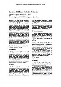
Example 1. We next give an example, to compare the bounds of Corollary 16, Theorem 17 and Proposition 18. Consider the following finite matrices of dimension 3 × 4: −4 5 −3 3 −2 3 −3 −3 (54) A = −4 1 2 −2 , B = 2 0 −1 4 0 2 −3 −1 5 −1 5 −1 From the graph of spectral function, Figure 1, it follows that the only eigenvalue is −2. The interval [−r(A] B), r(B ] A)] is in this case [−2, 0.5]. Bounds (51) of [CGB08, Theorem 2.1] yield the interval [D(A, B), D(A, B)] = [−3, 2], which is less precise. Proposition 18 yields the union of intervals [3, 0] = ∅, [−2, −2], [3, 3] and [−3, −2], thus
THE LEVEL SET METHOD FOR THE TWO-SIDED MAX-PLUS EIGENPROBLEM
17
[−3, −2] ∪ {3}. Note that these intervals are incomparable both with [−r(A] B), r(B ] A)] and [D(A, B), D(A, B)] = [−3, 2]. We remark that the intervals [− ∨i (A] B0)i , ∨i (B ] A0)i ] and [D(A, B), D(A, B)] are also in general incomparable. Also, Subsect. 3.5 will provide an example where the bounds [−r(A] B), r(B ] A)] are exact. 3.3. Asymptotics of the spectral function. If A and B do not have −∞ columns, the functions λ + A] B and −λ + B ] A are represented as infima of all max-linear mappings (p) (s) Kλ and, respectively, Mλ such that (p)
(Kλ )i· = λ − aki + Bk· ,
(55)
1 6 k 6 n, aki 6= −∞,
(s)
(Mλ )i· = −λ − bki + Ak· ,
1 6 k 6 n, bki 6= −∞.
This representation satisfies the selection property. (p) (s) (p) Matrices Kλ and Mλ are both instances of Hλ which represent hλ . The spectral radii (p) r(Hλ ) are maximum cycle means expressed by λk1 /l1 + α, where 0 6 |k1 | 6 l1 6 m. The coefficient k1 /l1 will be called slope and α will be called offset. In fact, it is only possible that k1 = l1 − 2t for t = 1, . . . , l1 , since all entries in the representing matrices are weighted with ±λ and only even numbers of ±λ terms can cancel out. As the arithmetic mean does not exceed the maximum, it follows that α 6 ∆(A, B), where _ _ (bij − aik ). (aij − bik ) ∨ (56) ∆(A, B) := i,j,k : bij 6=−∞, aik 6=−∞
i,j,k : aij 6=−∞, bik 6=−∞
We also define
_
C(A, B) := (57)
(aij − bik ),
i,j,k : aij 6=−∞, bik 6=−∞
^
C(A, B) :=
(aik − bij ).
i,j,k : aik 6=−∞, bij 6=−∞
Using these observations and notation we study the asymptotics of s(λ), both in general case and in some special cases. Theorem 19. Suppose that A, B ∈ Rn×m max . 1. Either s(λ) = −∞ for all λ, or there exist k1 , l1 , k2 , l2 such that 0 6 l1 6 m, k1 = l1 −2t1 where 0 6 t1 6 bl1 /2c, 0 6 l2 6 m, k2 = l2 −2t2 where 0 6 t2 6 bl2 /2c, and α1 , α2 ∈ R such that (58)
s(λ) = λk1 /l1 + α1 ,
if λ 6 −2m2 × ∆(A, B),
s(λ) = −λk2 /l2 + α2 . if λ > 2m2 × ∆(A, B).
18
´ STEPHANE GAUBERT AND SERGE˘I SERGEEV
2. Suppose that A and B do not have −∞ columns. Then either s(λ) = −∞ for all λ, or there exist α1 6 r(A] B) and α2 6 r(B ] A) such that (59)
s(λ) = λ + α1 , s(λ) = −λ + α2 ,
if λ 6 −2m × ∆(A, B), if λ > 2m × ∆(A, B).
3. Suppose that A and B are real. Then (60)
s(λ) = λ + r(A] B), s(λ) = −λ + r(B ] A),
if λ 6 C(A, B), if λ > C(A, B).
Proof. 1: For the proof of this part, we observe that for each λ, the function s(λ) is the (p) maximum cycle mean of a certain representing matrix Hλ , so that it equals λk/l + α where 0 6 l 6 m, k = l − 2t where 0 6 t 6 l. For any two such terms, difference between coefficients k/l is not less than 1/m2 , and the difference between the offsets does not exceed 2∆(A, B), which yields that all intersection points must be in the interval [−2m2 × ∆(A, B), 2m2 × ∆(A, B)]. Thus s(λ) is linear for λ 6 −2m2 × ∆(A, B) and for λ > 2m2 × ∆(A, B). As s(λ) 6 0 for all λ, the left asymptotic slope is nonnegative, and the right asymptotic slope is non-positive. (p) (p) 2: When A does not have −∞ columns, some of the matrices Hλ are of the form Kλ (p) and their maximum cycle mean is λ + α. Taking minimum over all r(Hλ ) of that form yields an offset α1 6 r(A] B). The cycle mean λ + α1 will dominate at small λ, and the smallest intersection point may occur with a term λ(m−1)/m+α10 . Indeed, the difference between coefficients is precisely the smallest possible 1/m, and the difference |α1 − α10 | may be up to 2∆(A, B). This yields the bound −2m × ∆(A, B). An analogous argument follows when λ is large and B does not have −∞ columns. 3: When A and B are real and λ < C(A, B), all coefficients in the min-max function λ + A] B are real negative, and all coefficients in the min-max function −λ + B ] A are real (p) positive. This implies that s(λ) is equal to the minimum over r(Kλ ), which is equal to λ + r(A] B). An analogous argument follows when λ > C(A, B). ¤ In Proposition 23 we will show by an explicit construction that any slope k/l can be realized as asymptotics of a spectral function. We next observe that the asymptotics of s(λ) can be read off from s◦ (λ), which is the spectral function associated with A◦ and B ◦ . These matrices were defined in (49), they have 0 entries exactly where A, resp. B, have finite entries.
THE LEVEL SET METHOD FOR THE TWO-SIDED MAX-PLUS EIGENPROBLEM
19
Proposition 20. Suppose that A, B ∈ Rn×m max and that that λk1 /l1 where k1 , l1 > 0 (resp. −λk2 /l2 where k2 , l2 > 0) is the left (resp. the right) asymptotic slope of s(λ). Then λk /l , if λ 6 0, 1 1 (61) s◦ (λ) = −λk2 /l2 , if λ > 0. (p◦)
Proof. Observe that the representing matrices Hλ (62)
of
h◦λ := (λ + (A◦ )] B ◦ x) ∧ (−λ + (B ◦ )] A◦ x) (p)
are in one-to-one correspondence with the representing matrices Hλ of hλ . The finite ◦(p) entries Hλ equal to ±λ, they are in the same places and with the same sign of λ as in (p) ◦(p) Hλ . Hence the cycle means in Hλ have the same slopes as the corresponding cycle (p) means in Hλ , but with zero offsets. When s(λ) = r(hλ ) is computed by (45), the asymptotics at large and small λ is determined by the slopes only and yields the same expression as for s◦ (λ) = r(h◦λ ). ¤ 3.4. Reconstructing the spectrum and the spectral function. Now we consider the problem of identifying all linear pieces that constitute the spectral function and computing the whole spectrum of (A, B) in the case when A and B have integer entries. The result will be formulated in terms of calls to an oracle computing the value of s(λ) at a given point. Essentially, this oracle computes the value of associated mean payoff game parametrized by λ. The role of such an oracle can be played by the policy iteration algorithm of [CTGG99, DG06]. Theorem 21. Let A, B ∈ Rn×m max have only integer or −∞ entries. 1. All linear pieces that constitute the function s(λ) and hence the spectrum of (A, B) can be identified in no more than ∆(A, B) × O(m6 ) calls to the oracle. 2. When A and B have no −∞ columns, the number of calls needed to reconstruct the function s(λ) can be decreased to ∆(A, B) × O(m5 ). When A and B are real, it is decreased to (C(A, B) − C(A, B)) × O(m4 ). Proof. In all cases we have a finite interval of length L, which is L := ∆(A, B) × O(m2 ) in case 1, and L = ∆(A, B) × O(m) or L := (C(A, B) − C(A, B)) in case 2. We first compute the asymptotic slopes of s(λ) outside L. By Proposition 20, we can do this by computing s◦ (±1) in just two calls to the oracle. Then the goal is to reconstruct all linear pieces which constitute s(λ) in the interval L. The linear pieces of s(λ) correspond to the maximal cycle means in the matrices from the representation of hλ (x). The points where such linear pieces may intersect are given
20
´ STEPHANE GAUBERT AND SERGE˘I SERGEEV
by (63)
a 1 + k1 λ a2 + k2 λ = , n1 n2
where all parameters are integers and 1 6 |k1 |, |k2 |, n1 , n2 6 m. This implies (64)
λ=
a1 n2 − a2 n1 k2 n 1 − k1 n 2
The denominators of these points range from −m2 to m2 , hence their number in the interval L is L × O(m4 ). We reconstruct the whole spectral function by calculating s(λ) at these points, since s(λ) is linear between them. ¤ Since spec(A, B) is the zero set of s(λ), we can identify spec(A, B) by reconstructing s(λ) in the spectral intervals given by Proposition 18. This yields the following Corollary 22. Let A, B ∈ Rn×m max have only integer or −∞ entries and no −∞ columns. Then the number of calls to the oracle needed to identify spec(A, B) does not exceed (∨i (B ] A0)i + ∨i (A] B0)i ) × O(m4 ). 3.5. Examples of analytic computation. In this section we consider two particular situations when the spectral function can be constructed analytically. The first example shows that any asymptotics k/l, where l = 1, . . . , m and k = l − 2t for t = 1, . . . , l, can be realized. The second example is taken from [Ser], and it shows that any system of intervals and points on the real line can be represented as spectrum of a max-plus two-sided eigenproblem. Asymptotic slopes. In our first example we consider pairs of matrices Am,l ∈ m,l Rm×m ∈ Rm×m max , B max with (0, −∞) entries, where 0 6 l 6 bmc. An intuitive idea is to make a certain “exchange” between the max-plus identity matrix and a certain cyclic permutation matrix. For instance · · · · · 0 0 · · · · · · 0 · · · · 0 · · · · · · 0 · · · · 6,2 · · 0 · · · 6,2 A = (65) · · · 0 · · , B = · · 0 · · · , · · · 0 · · · · · · 0 · · · · · 0 · · · · · · 0 where the dots denote −∞ entries. m,l Formally, Am,l = (am,l ij ) are defined as matrices with {0, −∞} entries such that aij = 0 for i = 1 and j = m, or i = j + 1 where 2l < i 6 m, or i = j = 2k where 1 6 k 6 l, or i = 2k + 1 and j = 2k, where 1 6 k < l, and am,l ij = −∞ otherwise.
THE LEVEL SET METHOD FOR THE TWO-SIDED MAX-PLUS EIGENPROBLEM
21
m,l Similarly, B m,l = (bm,l ij ) are defined as matrices with {0, −∞} entries such that bij = 0 for i = j where 2l < i 6 m, or i = j = 2k − 1 where 1 6 k 6 l, or i = 2k and j = 2k − 1, where 1 6 k 6 l, and bm,l ij = −∞ otherwise.
Proposition 23. The spectral function associated with Am,l , B m,l consists of two linear pieces: s(λ) = λ × (m − 2l)/m for λ 6 0 and s(λ) = −λ × (m − 2l)/m for λ > 0. m×m Proof. Let us introduce yet another matrix C m,l (λ) = (cm,l ij (λ)) ∈ Rmax . Informally, it is a sum of a {0, −∞} permutation (circulant) matrix and its inverse, weighted by ±λ. This pattern corresponds to the above mentioned “exchange” in the construction of Am,l and B m,l . In particular, (65) corresponds to · −λ · · · −λ · · λ · λ · · −λ · −λ · · 6,2 . (66) C = · · λ · λ · · · · −λ · λ λ · · · −λ · m,l Defining formally, cm,l 1,m = −λ, cm,1 = λ, and sign(i, j) × λ, if 1 6 i, j 6 m and |j − i| = 1, m,l (67) cij = −∞, otherwise,
where (68)
1, j − 1 = i > 2l or j ± 1 = i = 2k 6 2l, sign(i, j) = −1, i − 1 = j > 2l or i ± 1 = j = 2k 6 2l.
Observe that the pairs (i, j) and (j, i) for j = i + 1 (and also (1, m) and (m, 1)) have the opposite sign. It can be shown that each representing max-plus matrix of the min-max function (69)
m,l ] m,l hm,l ) B x) ∧ (−λ + (B m,l )] Am,l x) λ (x) = (λ + (A
is choosing one of the two entries in each row of C m,l (λ). The matrices can be classified according to this choice as follows (see (66) for an illustration): 1. Choose (m, 1), and (i, i + 1) for i = 1, . . . , m − 1; 2. Choose (1, m), and (i, i − 1) for i = 2, . . . , m; 3. Choose both (m, 1) and (1, m), or both (i − 1, i) and (i, i − 1) for some i = 2, . . . , n. The first two strategies give just one matrix each, with the (maximum) cycle means λ × (m − 2l)/m and −λ × (m − 2l)/m. The rest of the representing matrices are described
22
´ STEPHANE GAUBERT AND SERGE˘I SERGEEV
by 3., and it follows that their maximum cycle means are always greater than or equal to 0. Hence s(λ) = λ × (m − 2l)/m ∧ −λ × (m − 2l)/m. ¤ The spectrum of two-sided eigenproblem. Now we consider an example of [Ser]. 2×3t Let us define A ∈ Rmax , B ∈ R2×3t max : Ã ! . . . ai bi ci . . . A= , . . . 2ai 2bi 2ci . . . (70) Ã ! ... 0 0 0 ... B= , . . . ai ci bi . . . where ai 6 ci < ai+1 for i = 1, . . . , t − 1, where bi := spec(A, B).
ai +ci . 2
The following result describes
Theorem 24 ([Ser]). With A, B defined by (70), (71)
spec(A, B) =
t [
[ai , ci ].
i=1
To calculate s(λ), which is a more general task, one can study the representing matrices like in the previous example. Another way is to guess, for each λ, a finite eigenvector of PD ◦ PC(λ) and then s(λ) is the corresponding eigenvalue. By this method we obtained that: λ − a1 , if λ 6 a1 , 0, if ak 6 λ 6 ck , k = 1, . . . , t, s(λ) = (72) max(ck − λ, λ − ak+1 ), if ck 6 λ 6 ak+1 , k = 1, . . . , t − 1, ct − λ, if λ > ct . More precisely, it (0 (0 (73) y λ = (0 (0 (0
can be shown that the following vectors are eigenvectors of PD PC(λ) : a1 0 a1 ),
if λ 6 a1 ,
λ + bk − ak 0 λ + bk − ak ),
if ak 6 λ 6 bk , k = 1, . . . , t,
ck 0 ck ),
if bk 6 λ 6 ck , k = 1, . . . , t,
λ 0 λ),
if ck 6 λ 6 ak+1 , k = 1, . . . , t − 1,,
ct 0 ct )T ,
if λ > ct ,
with the eigenvalues expressed by (72). We can also conclude that in this case −r(A] B) = a1 and r(B ] A) = ct . Indeed, by (72), s(λ) = λ − a1 for λ 6 a1 and s(λ) = ct − λ for λ > ct . Comparing this with the result of Theorem 19, part 3, we get the claim.
THE LEVEL SET METHOD FOR THE TWO-SIDED MAX-PLUS EIGENPROBLEM
23
0 −0.1 −0.2 −0.3 −0.4 −0.5 −0.6 −0.7 −0.8 −0.9 −1
0
0.5
1
1.5
2
2.5
3
3.5
4
Figure 2. The spectral function of A and B in (74) As a1 and ct are eigenvalues, the last result shows that the bounds given in Theorem 17 cannot be improved in general. Example 2. In (70), take t = 3, [a1 , c1 ] = [1, 2], Then à 1 1.5 2 2.2 A= 2 3 4 4.4 (74) à 0 0 0 0 B= 1 2 1.5 2.2
[a2 , c2 ] = [2.2, 2.4] and [a3 , c3 ] = [3, 3]. ! 2.3 2.4 3 , 4.6 4.8 6 ! 0 0 0 2.4 2.3 3
The spectral function is shown on Figure 2. Acknowledgement. The authors thank Peter Butkoviˇc and Hans Schneider for many useful discussions which have been at the origin of this work. References [ABG98]
M. Akian, R. Bapat, and S. Gaubert. Asymptotics of the perron eigenvalue and eigenvector
[ABG04]
using max-algebra. C.R.A.S. Serie I, 327:927–932, 1998. M. Akian, R. Bapat, and S. Gaubert. Perturbation of eigenvalues of matrix pencils and
[ABG06a]
optimal assignment problem. C.R.A.S. Serie I, 339:103–108, 2004. arXiv:math.SP/0402438. M. Akian, R. Bapat, and S. Gaubert. Min-plus methods in eigenvalue perturbation theory and generalized Lidski˘ı-Viˇsik-Ljusternik theorem. E-print arXiv:math/0402090v3, 20042006.
24
[ABG06b]
[AGG09] [AGK05]
[BCOQ92] [BHAB95]
[Bur91] [But03] [BV07] [CG79] [CGB03] [CGB08]
[CGQS05]
[CTGG99] [DG06]
[DS04] [GG98a]
´ STEPHANE GAUBERT AND SERGE˘I SERGEEV
M. Akian, R. Bapat, and S. Gaubert. Max-plus algebras. In L. Hogben, editor, Handbook of Linear Algebra (Discrete Mathematics and Its Applications), volume 39. Chapman & Hall/CRC, 2006. Chapter 25. M. Akian, S. Gaubert, and A. Guterman. Tropical polyhedra are equivalent to mean payoff games. Eprint arXiv:0912.2462, 2009. M. Akian, S. Gaubert, and V. Kolokoltsov. Set coverings and invertibility of the functional galois connections. In G. Litvinov and V. Maslov, editors, Idempotent Mathematics and Mathematical Physics, volume 377, pages 19–51. American Mathematical Society, Providence, 2005. E-print arXiv:math.FA/0403441. F. L. Baccelli, G. Cohen, G. J. Olsder, and J. P. Quadrat. Synchronization and Linearity: an Algebra for Discrete Event Systems. Wiley, 1992. S. M. Burns, H. Hulgaard, T. Amon, and G. Borriello. An algorithm for exact bounds on the time separation of events in concurrent systems. IEEE Transactions on Computers, 44(11):1306–1317, 1995. S.M. Burns. Performance analysis and optimization of asynchronous circuits. PhD thesis, California Institute of Technology, 1991. P. Butkoviˇc. Max-algebra: the linear algebra of combinatorics? Linear Algebra Appl., 367:313–335, 2003. P.A. Binding and H. Volkmer. A generalized eigenvalue problem in the max algebra. Linear Algebra Appl., 422:360–371, 2007. R. A. Cuninghame-Green. Minimax Algebra, volume 166 of Lecture Notes in Economics and Mathematical Systems. Springer, Berlin, 1979. R.A. Cuninghame-Green and P. Butkoviˇc. The equation a ⊗ x = b ⊗ y over (max,+). Theoretical Computer Science, 293:3–12, 2003. R.A. Cuninghame-Green and P. Butkoviˇc. Generalised eigenproblem in max algebra. In Proceedings of the 9th International Workshop WODES 2008, pages 236–241, 2008. http://ieeexplore.ieee.org/stamp. G. Cohen, S. Gaubert, J. P. Quadrat, and I. Singer. Max-plus convex sets and functions. In G. Litvinov and V. Maslov, editors, Idempotent Mathematics and Mathematical Physics, volume 377 of Contemporary Mathematics, pages 105–129. AMS, Providence, 2005. E-print arXiv:math.FA/0308166. J. Cochet-Terrasson, S. Gaubert, and J. Gunawardena. A constructive fixed-point theorem for min-max functions. Dynamics and Stability of Systems, 14(4):407–433, 1999. V. Dhingra and S. Gaubert. How to solve large scale deterministic games with mean payoff by policy iteration. In Proceedings of the 1st international conference on Performance evaluation methodolgies and tools (VALUETOOLS), volume 180, Pisa, Italy, 2006. article No. 12. M. Develin and B. Sturmfels. Tropical convexity. Documenta Math., 9:1–27, 2004. E-print arXiv:math.MG/0308254. S. Gaubert and J. Gunawardena. The duality theorem for min-max functions. C. R. Acad. Sci. Paris., 326, S´erie I:43–48, 1998.
THE LEVEL SET METHOD FOR THE TWO-SIDED MAX-PLUS EIGENPROBLEM
[GG98b]
25
S. Gaubert and J. Gunawardena. A non-linear hierarchy for discrete event dynamical sys-
tems. In Proc. of the Fourth Workshop on Discrete Event Systems (WODES98), Cagliari, Italy, 1998. IEE. [GK09] S. Gaubert and R. D. Katz. The tropical analogue of polar cones. Linear Algebra Appl., 431(5-7):608–625, 2009. E-print arXiv:0805.3688. [GS08] S. Gaubert and S. Sergeev. Cyclic projectors and separation theorems in idempotent convex geometry. Journal of Math. Sci., 155(6):815–829, 2008. E-print arXiv:math/0706.3347. [Gun94] J. Gunawardena. Min-max functions. Discrete Event Dynamic Systems, 4:377–406, 1994. [HOvdW05] B. Heidergott, G.-J. Olsder, and J. van der Woude. Max-plus at Work. Princeton Univ. [KM97] [LL69] [LMS01]
Press, 2005. V. N. Kolokoltsov and V. P. Maslov. Idempotent analysis and its applications. Kluwer Academic Pub., 1997. T. M. Liggett and S. A. Lippman. Stochastic games with perfect information and time average payoff. SIAM Rev., 11:604–607, 1969. G. L. Litvinov, V. P. Maslov, and G. B. Shpiz. Idempotent functional analysis: An algebraic approach. Math. Notes (Moscow), 69(5):758–797, 2001.
[Min88] [MNV08]
H. Minc. Nonnegative matrices. Wiley, 1988. V. Mehrmann, R. Nabben, and E. Virnik. Generalization of Perron-Frobenius theory to matrix pencils. Linear Algebra Appl., 428:20–38, 2008.
[MOS+ 98]
J. J. McDonald, D. D. Olesky, H. Schneider, M. J. Tsatsomeros, and P. van den Driessche. Z-pencils. Electronic J. Linear Algebra, 4:32–38, 1998. R. H. M¨ohring, M. Skutella, and F. Stork. Scheduling with AND/OR precedence constraints. SIAM J. Comput., 33(2):393–415 (electronic), 2004. R.D. Nussbaum. Convexity and log convexity for the spectral radius. Linear Algebra Appl., 73:59–122, 1986.
[MSS04] [Nus86] [Ols91] [Ser] [Ser09]
[ZP96]
G.J. Olsder. Eigenvalues of dynamic min-max functions. Discrete Event Dynamic Systems, 1:177–207, 1991. S. Sergeev. Spectrum of two-sided eignproblem in max algebra: every system of intervals is realizable. Submitted to Discrete Appl. Math., E-print arXiv:1001.4051, 2010. S. Sergeev. Multiorder, Kleene stars and cyclic projectors in the geometry of max cones. In G. L. Litvinov and S. N. Sergeev, editors, Tropical and Idempotent Mathematics, volume 495 of Contemporary Mathematics, pages 317–342. AMS, Providence, 2009. E-print arXiv:0807.0921. U. Zwick and M. Paterson. The complexity of mean payoff games on graphs. Theoretical Computer Science, 158(1-2):343–359, 1996.
26
´ STEPHANE GAUBERT AND SERGE˘I SERGEEV
´ ´matiques Applique ´es,Ecole INRIA and Centre de Mathe Polytechnique. Postal ad´ ´ dress: CMAP, Ecole Polytechnique, 91128 Palaiseau Cedex, France. E-mail address:
[email protected] University of Birmingham, School of Mathematics, Watson Building, Edgbaston B15 2TT, UK E-mail address:
[email protected]