The Locality of Distributed Symmetry Breaking

The Locality of Distributed Symmetry Breaking∗ Leonid Barenboim

Michael Elkin

Seth Pettie

Johannes Schneider

arXiv:1202.1983v3 [cs.DC] 24 Feb 2015

February 26, 2015

Abstract Symmetry breaking problems are among the most well studied in the field of distributed computing and yet the most fundamental questions about their complexity remain open. In this paper we work in the LOCAL model (where the input graph and underlying distributed network are identical) and study the randomized complexity of four fundamental symmetry breaking problems on graphs: computing MISs (maximal independent sets), maximal matchings, vertex colorings, and ruling sets. A small sample of our results includes √

• An MIS algorithm running in O(log2 ∆ + 2O( log log n) ) time, where ∆ is the maximum degree. This is the first MIS algorithm to improve on the 1986 algorithms of Luby and √ Alon, Babai, and Itai, when log n ∆ 2 log n , and comes close to the Ω(log ∆) lower bound of Kuhn, Moscibroda, and Wattenhofer. • A maximal matching algorithm running in O(log ∆ + log4 log n) time. This is the first significant improvement to the 1986 algorithm of Israeli and Itai. Moreover, its dependence on ∆ is provably optimal. √ • A (∆ + 1)-coloring algorithm requiring O(log ∆ + 2O( log log n) ) time, improving on an √ O(log ∆ + log n)-time algorithm of Schneider and Wattenhofer. • A method for reducing symmetry breaking problems in low arboricity/degeneracy graphs to low degree graphs. (Roughly speaking, the arboricity or degeneracy of a graph bounds √ log n)-time the density of any subgraph.) Corollaries of this reduction include an O( √ maximal matching algorithm for graphs with arboricity up to 2 log n and an O(log2/3 n)1/3 time MIS algorithm for graphs with arboricity up to 2(log n) . Each of our algorithms is based on a simple, but powerful technique for reducing a randomized symmetry breaking task to a corresponding deterministic one on a poly(log n)-size graph.

1

Introduction

Breaking symmetry is one of the central themes in the theory of distributed computing. At initialization the nodes of a distributed system are assumed to be in the same state, possibly with distinct ∗

A preliminary version of this paper appeared in the Proceedings of the 53rd IEEE Symposium on Foundations of Computer Science (FOCS), 2012. This work is supported by NSF grants CCF-0746673, CCF-1217338, and CNS1318294, US-Israel Binational Science Foundation grant 2008390, and Israeli Academy of Science grant 593/11. This research was partly performed while S. Pettie was on sabbatical at the Center for Massive Data Algorithmics (MADALGO), Aarhus University, which is supported by Danish National Research Foundation grant DNRF84. Author’s addresses: Leonid Barenboim, Department of Mathematics and Computer Science, The Open University of Israel; Michael Elkin, Department of Computer Science, Ben-Gurion University; Seth Pettie (corresponding author), Department of Electrical Engineering and Computer Science, University of Michigan; Johannes Schneider, ABB Research, Z¨ urich.

1

node IDs, yet to perform any computation the nodes frequently must take different roles. That is, they must somehow break their initial symmetry. In this paper we study several of the most fundamental symmetry breaking tasks in the LOCAL model [27]: computing maximal independent sets (MIS), maximal matchings, ruling sets, and vertex colorings. These problems are defined below. In the LOCAL model each node of the input graph G hosts a processor, which is only aware of its neighbors and upper bounds on various graph parameters such as n and ∆, which are the number of nodes and maximum degree, respectively.1 The computation proceeds in synchronized rounds in which each processor sends one unbounded message along each edge. Time is measured by the number of rounds; local computation is free. At the end of the computation each node must report its portion of the output, that is, whether it is in the MIS or ruling set, which incident edge is part of the matching, or its assigned color. This model should be contrasted with CONGEST, which is identical to LOCAL except messages consist of O(1) words, that is, O(log n) bits. Refer to Peleg [33, Ch. 1-2] for a discussion of distributed models. None of our algorithms seriously abuse the power of the LOCAL model. Our message size and local computation are always O(poly(∆) log n), usually O(poly(log n)), and in several cases O(1). Let us define the four problems formally. Maximal Independent Set Given G = (V, E), find any set I ⊆ V such that no two nodes in I are adjacent and I is maximal with respect to inclusion. (That is, every v 6∈ I is adjacent to some member of I.) (α, β)-Ruling Set Given G(V, E), find any R ⊂ V such that for every u ∈ V , dist(u, R) ≤ β and for every u ∈ R, dist(u, R\{u}) ≥ α. Note that (2, 1)-ruling sets are maximal independent sets. (Here dist(u, X) is the length of a shortest path from u to any member of X.) Maximal Matching Given G = (V, E), find any matching M ⊆ E (consisting of node-disjoint edges) that is maximal with respect to inclusion. K-Coloring Given G = (V, E), find a proper coloring Color : V → {1, . . . , K}, that is, one for which (u, v) ∈ E implies Color(u) 6= Color(v). We are mainly interested in (∆ + 1)-colorings, whose existence is trivially guaranteed. We study the complexities of these problems on general graphs, as well as graphs with a specified arboricity λ. By definition λ(G) is the minimum number of edge-disjoint forests that cover E, which is roughly the maximum density of any subgraph. We believe arboricity is an important graph parameter as it robustly captures the notion of sparsity without imposing any strict structural constraints, such as planarity or the like. We always have λ ≤ ∆, but in general λ could be significantly smaller than ∆. Most sparse graph classes, for example, have λ = O(1) though their maximum degree is unbounded. These include planar graphs (λ = 3), graphs avoiding a fixed minor, bounded genus graphs, and graphs of bounded treewidth or pathwidth. However, none of our algorithms actually depend on having λ = O(1). 1 This assumption can sometimes be removed. Korman, Sereni, and Viennot [19] presented a method to convert non-uniform distributed algorithms (which know n, ∆, and possibly other parameters) into uniform distributed algorithms.

2

1.1

The State of the Art in Distributed Symmetry Breaking

The reader will soon notice two striking features of prior research on distributed symmetry breaking: the wide gulf between the efficiency of deterministic and randomized algorithms and the paltry number of algorithms that are provably optimal. It is typical to see randomized algorithms that are exponentially faster (in terms of n or ∆) than their deterministic counterparts, and they are usually simpler to analyze and simpler to implement. Very few problems can be solved in O(1) time, independent of ∆ and n. The ω(1) lower bounds of Linial [27] and Kuhn, Moscibroda, and Wattenhofer [24] are known to be tight in only a few cases, typically on very special classes of graphs. We survey lower bounds and algorithms for each of the symmetry breaking problems below. Tables 1–4 provide an at-a-glance history of the problems. In the tables, deterministic algorithms are indicated by Det. All other algorithms are randomized, which return a correct answer with high probability.2 Lower Bounds Linial [27] proved that log(k) n-coloring the n-cycle takes Ω(k) time, and therefore that O(1)-coloring the n-cycle takes Ω(log∗ n) time. On the n-cycle, MIS, maximal matching, and ruling sets are equivalent to O(1)-coloring, so Linial’s lower bound applies to these problems as well. Kuhn, Moscibroda, and Wattenhofer [24]√(henceforth, KMW) proved that O(1)-approximate minimum vertex cover (MVC) takes Ω(min{ log n, log ∆}) time. Since 2-approximate MVC is reducible to maximal matching and maximal matching is reducible to MIS (on the line graph of √ the original graph), the KMW lower bound implies Ω(min{ log n, log ∆}) lower bounds on these problems as well. It does not apply to coloring problems, nor the (α, β)-ruling set problem except when (α, β) = (2, 1). √

Deterministic MIS The fastest deterministic MIS algorithms for general graphs run in 2O( log n) time [32] and O(∆ + log∗ n) time [8]. The Panconesi-Srinivasan [32] result is actually a network √ deO( log n) composition algorithm, which can be used to solve many symmetry breaking problems in 2 √ time. It improved on an earlier algorithm of Awerbuch et al. [4] running in 2O( log n log log n) time. Recent work on deterministic MIS algorithms has focussed on restricted graph classes. Schneider and Wattenhofer [37] gave an optimal O(log∗√n)-time MIS algorithm for growth-bounded graphs.3 Barenboim and Elkin [5, 7] gave an O(λ log n + log n)-time MIS algorithm, and anlog n 1/2−δ . The subsequent vertex other that runs in O( δ log log n ) when the arboricity is λ = (log n) coloring algorithms of Barenboim and Elkin [6] give, as corollaries, MIS algorithms running in O(λ + min{λ log n, log1+ n}) time and O(λ1+ + log λ log n) time, where > 0 influences the leading constants. Randomized MIS Nearly 30 years ago Luby [29] and Alon, Babai, and Itai [2] presented very simple randomized MIS algorithms running in O(log n) time. These algorithms are faster than the best deterministic algorithms when ∆ = ω(log n) and remain the fastest MIS algorithms for general graphs when running time is expressed solely as a function of n. Lenzen and Wattenhofer [26] 2 An event occurs with high probability if its probability is at least 1 − n−c for an arbitrarily large c, where c may influence other constants, for example, those hidden in asymptotic running times. 3 A graph class has bounded growth if for each v ∈ V and radius r, the maximum size of an independent set in v’s r-neighborhood is a constant depending on r. For example, unit-disc graphs have bounded growth.

3

√ showed that in the special case of trees (λ = 1), an MIS can be computed in O( log n log log n) time with high probability.4 Deterministic Maximal Matching √ Panconesi and Srinivasan’s [32] network decomposition algorithm implies a deterministic 2O( log n) -time maximal matching algorithm. This bound was dramatically improved by Ha´ nćkowiak, Karo´ nski, and Panconesi [16] to O(log4 n). When ∆ = o(log4 n), maximal matchings can be computed faster, in O(∆+log∗ n) time, using the algorithm of Panconesi and Rizzi [31]. Barenboim and Elkin [5, 7] gave improved algorithms for low arboricity log n graphs. Their algorithms run in O(λ + log n) time, for any λ, and in O( δ log log n ) time when 1−δ λ = log n. Randomized Maximal Matching Since a maximal matching in G is simply an MIS in the line graph of G, the randomized MIS algorithms of [29, 2] can be used to solve maximal matching in O(log n) time as well.5 Israeli and Itai [17] presented a direct randomized algorithm for computing maximal matchings in O(log n) time. This algorithm is faster than the deterministic algorithms when ∆ = ω(log n), and remains the fastest maximal matching algorithm whose running time is expressed solely as a function of n. Deterministic Vertex Coloring The vertex coloring problem allows for a tradeoff between the palette size (number of colors) and running time. Linial [27] proved that O(∆2 )-coloring can be computed deterministically in O(log∗ n) time, independent of ∆. Szegedy and Vishwanathan [38] later improved the running time of this algorithm to 21 log∗ n + O(1). The best deterministic √ (∆ + 1)-coloring algorithms run in 2O( log n) time [32] or O(∆ + log∗ n) time [8]. Even if the palette size is enlarged to O(∆), the Panconesi-Srinivasan [32] algorithm remains the fastest, when time is expressed as a function of n. However, Barenboim and Elkin [6] gave an O(min{λ log n, λ + log1+ n})-time algorithm for O(λ)-coloring, and an O(log λ log n)-time algorithm for λ1+ -coloring. (The hidden constants are exponential in 1/.) Since the arboricity λ is at most ∆, one can substitute ∆ for λ in the bounds cited above. Randomized Vertex Coloring As usual, significantly faster coloring algorithms can be obtained using randomization. Luby [29] gave a reduction from (∆ + 1)-coloring to MIS, which implies an O(log n) time randomized algorithm. A direct O(log n)-time (∆ + 1)-coloring algorithm was analyzed by Johansson [18]. By enlarging the √ palette, vertex coloring can be solved dramatically faster. Kothapalli et al. [22] showed that O( log n) time suffices √ for computing an O(∆)-coloring, for any ∆. Schneider and Wattenhofer [36] gave an O(log ∆ + log n)-time (∆ + 1)coloring algorithm, for any ∆, and several faster O(∆)-coloring algorithms when ∆ is sufficiently large. For example, when ∆ = Ω(log n), O(∆)-coloring can be computed in O(log log n) time and ∗ when ∆ = Ω(log1+1/ log n n), O(∆)-coloring can be computed in O(log∗ n) time. Kuhn and Wattenhofer [25] showed that O(∆ log n log(k) n)-coloring is computable in O(k) time and in particular, an O(∆ log2 n)-coloring could be computed in a single round. 4 5

See footnote 8. These simulations increase the local computation at each node.

4

Ruling Sets As noted earlier, an MIS is a (2, 1)-ruling set. More generally, an (α, (α−1)β)-ruling set can be found by computing a (2, β)-ruling set in the graph G[1,α−1] , whose edge set consists of pairs (u, v) for which distG (u, v) ∈ [1, α − 1]. (See Section 2 for details of graph notation.) A distributed algorithm in G[1,α−1] can be simulated in G with an (α − 1)-factor slowdown. This reduction changes various graph parameters so it is not always applicable. For example, ∆(G[1,α−1] ) is roughly (∆(G))α−1 and λ(G[1,α−1] ) cannot be bounded as a function of λ(G). Awerbuch, Goldberg, Luby, and Plotkin [4] gave a deterministic (2, log n)-ruling set algorithm running in O(log n) time. Schneider, Elkin, and Wattenhofer [35] recently discovered a (2, β)ruling set algorithm running in O(β∆2/β + log∗ n) time, for any integer parameter β, and another (2, β∆1/β ) ruling set algorithm running in O(β + log∗ n) time. These are the only deterministic ruling set algorithms. Using randomization, Gfeller and Vicari [15] showed that a (1, O(log log ∆))-ruling set could be computed such that the maximum degree in the graph induced by the ruling set is O(log5 n). Schneider and Wattenhofer [36] gave a randomized algorithm for computing a (2, β)-ruling set in O(2β/2 log2/(β−1) n) √time. This bound was improved by Bisht, Kothapalli, and Pemmaraju [10] to O(β log1/(β−1) ∆+2O( log log n) ) time. In earlier work, Kothapalli and Pemmaraju [21] gave a randomized (2, 2)-ruling set algorithm running in O(log1/2 ∆ · log1/4 n) time and a randomized (2, 3)-ruling set algorithm running in poly(log log n) time for graphs with arboricity λ = O(1).

1.2

The Union Bound Barrier

Our algorithms confront a fundamental barrier in randomized distributed algorithms we call the union bound barrier, which, to our knowledge, has never been explicitly discussed. Consider a generic symmetry breaking algorithm that works as follows. The nodes execute some number of iterations of an O(1)-time randomized experiment, the purpose of which is to commit to some fragment of the output. That is, some nodes are committed to the MIS or ruling set, some edges are committed to the matching, some nodes commit to a color, etc. The experiment fails at each node v with probability 1 − Ω(1). For example, failure may be defined as the event that no edge incident to v joins the matching. The failure events are not independent in general, but are independent for sufficiently distant nodes. If the random experiment takes t time steps, nodes at distance at least 2t+1 are influenced by disjoint sets of nodes. Although each node succeeds after Θ(1) time in expectation, the union bound only lets us claim that a global solution is reached with probability 1 − n−Ω(1) after Θ(log n) time. Symmetry breaking algorithms based on a random experiment with failure probability p seem intrinsically incapable of running in o(log1/p n) time.6 However, there are several conceivable strategies one could use to escape this conclusion. Among them, Use no randomness Deterministic algorithms have no probability of failure. Redefine failure If the experiment is kept the same but the notion of failure is relaxed such that it only occurs with probability n−Ω(1) , the union bound can be applied. We borrow an idea used in early constructive algorithms for the Lovász Local Lemma [9, 1] and more recently by [34], which combines elements from both of the strategies above. 6 Moreover, existing randomized algorithms [29, 2, 17] do not even fit in this framework. They do not guarantee each node succeeds with probability Ω(1), only that an Ω(1)-fraction of the edges are incident to nodes that succeed with probability Ω(1).

5

Maximal Independent Set Citation Linial [27] Kuhn, Moscibroda

Running Time

Graphs

∗

Ω(log n) Ω min

n-cycle

√

log n, log ∆

general

& Wattenhofer [24] Luby [29]

log n

general

Alon, Babai & Itai [2] √

Panconesi & Srinivasan [32] Barenboim, Elkin & Kuhn [8]

Barenboim & Elkin

[5, 6]

Schneider & Wattenhofer [37] Lenzen & Wattenhofer [26]

2O(

log n)

Det.

general

∆ + log∗ n

Det.

general

log n δ log log n

Det.

λ = log1/2−δ n

√ λ log n + log n

λ + min{λ log n, log1+ n} Det. λ1+ + log λ log n

Det.

log∗ n

Det.

√ log n log log n 2

log ∆ + 2O( 2

log ∆ +

√

2

log ∆ +

λ1+

log log n)

n

+ log λ log log n

log2 ∆ + λ + λ log log n log2 ∆ + λ + (log log n)1+ √ log n log log n log log n log log log n √ 2O( log log n)

log ∆ log log ∆ + log ∆ log log n + Table 1:

6

all λ, fixed > 0

bounded growth trees (λ = 1)

log log n δ log log log n 2/3

log2 λ + log

This paper

Det.

general λ = log1/2−δ log n all λ all λ, fixed > 0

trees (λ = 1) girth > 6

Maximal Matching Citation Linial [27] Kuhn, Moscibroda

Running Time

Graphs

∗

Ω(log n) Ω min

√

n-cycle log n, log ∆

general

& Wattenhofer [24] Israeli & Itai [17]

log n

Ha´ nćkowiak, Karo´ nski

log4 n

Det.

general

& Panconesi [16]

log3 n

Det.

bipartite

Panconesi & Rizzi [31]

∆ + log∗ n

Det.

general

log n δ log log n

Det.

λ = log1−δ n

λ + log n

Det.

all λ

Barenboim & Elkin [5]

This paper

general

log ∆ + log4 log n

general

log ∆ + log3 log n

bipartite

log log n log ∆ + δ log log log n √ log λ + log n

λ = log1−δ log n

log ∆ + λ + log log n Table 2:

7

all λ

Vertex Coloring Citation Linial [27] Cole & Vishkin [11]

Colors 3

Running Time Ω(log∗ n)

(on the n-cycle)

Luby [29]

Det.

log n

Johansson [18]

2O(

Panconesi & Srinivasan [32]

√

log n)

Det.

∗

∆ + log n √ log ∆ + log n

Barenboim, Elkin & Kuhn [8] Schneider & Wattenhofer [36]

log∗ n +O(1)

∆+1

√

log ∆ + 2O(

Det.

log log n)

log ∆ + λ1+ + log λ log log n log ∆ + λ + λ log log n log ∆ + λ + (log log n)1+

This paper

log ∆ + λ log log n

∆ + O(λ)

log ∆ + λ + (log log n)1+

∆ + λ1+

log ∆ + log λ log log n 2O(

Kothapalli, Scheideler, Onus & Schindelhauer [22]

√

O(∆)

√

log log n)

log n

min{∆ log n, ∆ + log1+ n} Det. Barenboim & Elkin [6]

Schneider & Wattenhofer [36] Kuhn & Wattenhofer [25] Linial [27] Szegedy & Vishwanathan [38] Barenboim & Elkin [5] Kothapalli & Pemmaraju [20]

O(λ)

min{λ log n, λ + log1+ n} Det.

∆1+

log ∆ log n

Det.

λ1+

log λ log n

Det.

O(∆ + log n) ∆ log + log

(k)

n

1+1/k

∆ log n log

n

(k)

n

O(∆2 ) λ · n1/k Table 3:

8

log log n k

(for k < log∗ n)

k

(for k < log∗ n)

log∗ n +O(1) 1 2

log n +O(1)

Ω(k) k

Det.

∗

(for log log n < k
∆/2k before the iteration, the probability that v ∈ Γ(I) after the iteration is at least −1/2 −1 (1 − e )e . ˆ IB (v) = {v = v0 , v1 , v2 , . . . , vdeg (v) } be the inclusive neighborhood of v. By assumpProof: Let Γ IB tion degIB (v) > ∆/2k and since v1 , . . . , vdegIB (v) were not marked bad (placed in B) in the last execution of Step 2b, degIB (vi ) ≤ ∆/2k−1 for each i ≤ degIB (v). Let i? ∈ {0, . . . , degIB (v)} be the first index for which b(vi? ) = 1. The probability that i? exists is degIB (v)

1−

Y i=0

13

1 1− degIB (vi ) + 1

≥1− 1−

∆/2k−1

def ˆ Recall that Γ(I) = I ∪ Γ(I) contains all vertices in or adjacent to I.

15

1

∆/2k +1

+1

> 1 − e−1/2 .

IndependentSet(Graph G) 1. Initialize sets I, B ⊂ V (G): I ←∅ {an independent set} B ←∅ {a set of ‘bad’ nodes} def ˆ ∪ B) be the nodes still under consideraThroughout, let VIB = V (G)\(Γ(I) tion: those not marked bad and not in or adjacent to the independent set. Let GIB be the graph induced by VIB and let ΓIB and degIB be the neighborhood and degree functions w.r.t. GIB .

2. For each scale k from 1 to log ∆ + 1, (a) Execute c log ∆ iterations of steps i and ii. i. Each node v ∈ VIB chooses a random bit b(v): (

1

with probability 1/(degIB (v) + 1)

0

with probability 1 − 1/(degIB (v) + 1)

b(v) ←

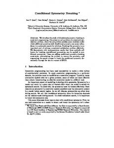
ii. I ← I ∪ {v ∈ VIB | b(v) = 1 and b(u) = 0 for all u ∈ ΓIB (v)}. (Add nodes to the independent set.) (b) B ← B ∪ {v ∈ VIB | degIB (v) > ∆/2k }. (Mark high-degree nodes as bad.) ˆ 3. B ← B\Γ(I). (Bad nodes adjacent to I no longer need to be considered bad.) 4. Return (I, B). Figure 1:

Figure 2: The node v0 is eliminated if some node in its inclusive neighborhood joins the independent set. This occurs if some vi? chooses b(vi? ) = 1 and 1 6∈ b(Γ(vi? )).

16

If i? does exist, vi? is included in the independent set I if all its neighbors set their b-values to zero. This occurs with probability Y 1 1 ∆/2k−1 1− ≥ 1− > e−1 . k−1 deg(u) + 1 ∆/2 +1 u∈ΓIB (vi? )\{v0 ,...,vi? −1 }

Nodes v0 , . . . , vi? −1 are excluded from consideration since, by definition of i? , they have already ˆ set their b-values to zero. Thus, after one iteration of Step 2a, v is in Γ(I) with probability −1/2 −1 (1 − e )e ≈ 0.145. See Figure 2 for an illustration. Lemma 3.2 Let U ⊂ V (G) be a node set such that distG (u, U \{u}) ≥ 5 for each u ∈ U . The probability that U ⊆ B after a call to IndependentSet(G) is less than ∆−c|U |/5 . ˆ Proof: The event that a node v ∈ VIB appears in Γ(I) after one iteration of Step 2a depends only on the random bits chosen by v’s neighbors and neighbors’ neighbors. Since all nodes in ˆ U are mutually at distance at least five, in each iteration the events that they appear in Γ(I) are independent. Call a node v ∈ VIB vulnerable in a particular iteration of Step 2a if degIB (v) > ∆/2k . We cannot say for certain when a node will be vulnerable, but eventually each must, for some k, ˆ be vulnerable throughout scale k, until it appears in Γ(I) or is placed in B at the end of the scale. By Lemma 3.1 the probability that an individual node ends up in B is at most pc log ∆ , where p = 1 − (1 − e−1/2 )e−1 ≈ 0.855. Since log p < −0.22, pc log ∆ = ∆c log p < ∆−c/5 . Since outcomes for U -nodes are independent in any iteration of Step 2a, the probability that every node in U ends up in B is at most ∆−c|U |/5 . Lemma 3.3 Let (I, B) be the pair returned by IndependentSet(G). For t = log∆ n, (I, B) satisfies the following properties with probability 1 − n−c/5+11 . 1. There does not exist any U ⊂ VIB with |U | = t such that for any U 0 ⊂ U , distG (U 0 , U \U 0 ) ∈ [5, 9]. 2. All components in the graph induced by VIB have fewer than t∆4 nodes. Proof: A set U ⊂ V satisfying the criteria of Part (1) forms a t-node tree in the graph G[5,9] . (This tree is not necessarily unique.) The number of rooted unlabeled t-node trees is less than 4t since the Euler tour of such a tree can be encoded as a bit-vector with length 2t. The number of ways to embed such a tree in G[5,9] is less than n · ∆9(t−1) : there are n choices for the root and less than ∆9 choices for each subsequent node. By Lemma 3.2 the probability that U ⊆ B is less than ∆−ct/5 . By a union bound, the probability that any such U is contained in B is less than 4t · n · ∆9(t−1) · ∆−ct/5 < nlog∆ 4+10−c/5 < n−c/5+11 . Turning to Part (2), suppose there is such a connected component C with t∆4 nodes. We can find a subset U of the nodes satisfying the criteria of Part (1) by the following greedy procedure. Choose an arbitrary initial node v1 ∈ C and set U ← {v1 }. Iteratively select a vi ∈ C\U for which distG (vi , U ) = 5, set U ← U ∪ {vi }, and then remove from consideration all nodes within distance 4 of vi . The number removed is less than ∆4 , hence U has size at least (t∆4 )/∆4 = t.

17

MIS(Graph G) Phase I: 1. (I, B) ← IndependentSet(G). The following steps focus on a single connected component C in GIB . They are executed in parallel for each such C. 2. (IC , BC ) ← IndependentSet(C). Phase II: ˆ C ) w.r.t. C. 3. RC ← a (5, 32 log ∆ + O(1))-ruling set for BC = V (C)\Γ(I 4. Form a cluster around each node x ∈ RC and form the cluster graph C ? .   Cluster(x) ← v ∈ BC 

 0 0 for any other x ∈ RC , distC (v, x) < distC (v, x )  or distC (v, x) = distC (v, x0 ) and ID(x) < ID(x0 ) 

C ← RC , (x, x0 ) ?

there exists (v, v 0 ) ∈ E(C) such that v ∈ Cluster(x) and v 0 ∈ Cluster(x0 )

√ √ 5. (D, C ) ← a 2O( log log n) , 2O( log log n) -network decomposition of C ? . 6. Compute the clustering of V (C) defined by D. For each D ∈ D, [ Cluster? (D) ← Cluster(x). x∈D

n o √ 7. For each color k ∈ 1, . . . , 2O( log log n) , (a) For each cluster D ∈ D with C (D) = k, in parallel, ˆ C ). JD ← an MIS of the graph induced by Cluster? (D)\Γ(I [ (b) IC ← IC ∪ JD . D∈D: C (D)=k

8. Return I ∪

[

IC .

C in GIB

Figure 3:

18

3.2

The MIS Algorithm

The pseudocode for MIS appears in Figure 3. We walk through each step of the algorithm below. Recall that IndependentSet(G) returns an independent set I and set of ‘bad’ nodes B. ˆ Step 1 After Step 1 we have an independent set I and a set of bad nodes B = VIB = V (G)\Γ(I). 4 By Lemma 3.3(2), with high probability each connected component in GIB has at most t · ∆ nodes and therefore at most t · ∆5 /2 edges, where t = log∆ n. Step 1 (and Step 2) require only 1-bit messages since each node only has to notify its neighbors about its status (whether in I or not, whether in VIB or not) and the b-values it selects in each round. Since the remaining steps operate on each component in GIB independently, messages of size O(∆5 log∆ n) suffice. Step 2

At this point we could simply run Panconesi and Srinivasan’s [32] deterministic MIS √ O log(t∆4 ) algorithm on each component. This would take time 2 , which is not the desired bound, unless ∆ happens to be polylogarithmic in n. In order to make this approach work for all ∆ we need to reduce the “effective” size of each component C to at most log n, independent of ∆. After ˆ C ) and BC . As we argue in the next paragraph, Step 2 we have partitioned V (C) ⊆ VIB into Γ(I Lemma 1 implies that BC (the bad nodes in C) can be efficiently partitioned into log n low-radius clusters. This is the only property of (IC , RC ) that we use in subsequent steps. Steps 3 and 4 Recall that nodes are assigned distinct O(log n)-bit IDs. Using Corollary 2.5 with α = 5, we can compute a (5, 32 log ∆ + O(1))-ruling set RC for BC in O(log ∆ + log∗ n) time. We form a cluster around each ruling set node in the obvious way: each v ∈ BC joins the cluster of the nearest x ∈ RC , called Cluster(x), breaking ties by node ID. Note that nearest is with respect to ˆ C ). The distC , so the shortest path from v to x does not leave C but may go through nodes in Γ(I ? cluster graph C is obtained by contracting each cluster Cluster(x) to a single node, also called x. We cannot use Lemma 3.3(1) directly to bound the size of RC since distC (v, RC \{v}) is only guaranteed to be at least 5, not in the interval [5, 9]. Consider a greedy procedure for obtaining a 0 ⊇ R . Initialize R0 ← R , then evaluate each u ∈ B , setting R0 ← R0 ∪ {u} (5, 4)-ruling set RC C C C C C C 0 . After this process completes, any u 6∈ R0 if u is at distance at least 5 from all vertices RC C 0 ) ≤ 4 and for any U 0 ⊂ R0 , dist (U 0 , R0 \U 0 ) ∈ [5, 9]. Thus, with probability has distC (u, RC C C C 0 | ≤ t. Note that the algorithm does not actually compute R0 . It was just 1 − n−c/5+11 , |RC | ≤ |RC C introduced to obtain an upper bound on |RC |. Steps 5 and 6 We run Panconesi and Srinivasan’s [32] decomposition algorithm on C ? . (See Remark 3.5, below, for a discussion of the subtle difficulties in implementing this algorithm.) Since √ √ O( log log n) O( log log n) |RC | ≤ t = log∆ n < log n we can compute a 2 ,2 -network decomposition √

(D, C ) in 2O( log log n) time. Since the underlying network is C, not C ? , each step of√this algorithm requires 64 log ∆+O(1) steps to simulate in C. The total time is therefore log ∆·2O( log log n) . Since Cluster? (D) is the union of disjoint clusters in {Cluster(x) | x ∈ D}, the diameter of Cluster? (D) √ O( log log n) . with respect to distC is at most (64 log ∆ + O(1)) · 2 Step 7 We extend IC to an MIS on C using the network decomposition. For each color class, for ˆ C ). These MISs are computed each cluster D, supplement IC with an MIS JD on Cluster? (D)/Γ(I

19

by the trivial algorithm and in parallel: a representative node in D retrieves the status of all nodes √ ? O( log log n) in Cluster (D), in O(log ∆ · 2 ) time, then computes an MIS JD and announces it to all nodes in Cluster? (D). At the end of this process IC is a maximal independent set on C. S Step 8 and Correctness The set returned in Step 8, I ∪ C IC , is usually an MIS of G. However, poor random choices in Steps 1 and 2 can cause the algorithm to fail during Step 5. The ruling set RC has size at most t with high probability. If itis larger than t then Steps3 and 4 will be executed √ √ without error, but Step 5 may fail to produce a 2O( log log n) , 2O( log log n) -network decomposition in the time allotted. If this occurs, Steps 6 and 7 cannot be executed. Running Time The time for Steps 1 and 2 is√O(log2 ∆) and the time for Steps 3 and 4 is O(log ∆+log∗√ n). Steps 5–7 take O(log ∆)·exp(O( log log n)) time. In total the time is O(log2 ∆+ √ log ∆ · exp(O( log log n))), which is O(log2 ∆ + exp(O( log log n))). Theorem in O(log2 ∆ + √ 3.4 In a graph with maximum degree ∆, an MIS can be computed exp(O( log log n))) time, with high probability, using messages with size O(∆5 log∆ n). Remark 3.5 One must be careful in applying deterministic algorithms in Phase II in a black box fashion. In the proof of Theorem 3.4 we reduced the number of clusters √ per component to t O( log t) time on each and deduced that the Panconesi-Srinivasan [32] algorithm runs in log ∆ · 2 component. This is not a correct inference. The stated running time of the Panconesi-Srinivasan algorithm depends on nodes being endowed with O(log t)-bit IDs (if the number of nodes is t), whereas in Step 5 nodes still have their original O(log n)-bit IDs. There is a simple generic fix for this problem. Suppose a deterministic Phase II algorithm A runs in time T = T (t) on any instance C with size t whose nodes are assigned distinct O(log t)-bit labels. Let k be minimal such that t ≥ log(k) n. Just before executing A, first compute an O(t2 log(k) n) = O(t3 )-coloring in the graph C [1,2T +1] with Linial’s [27] algorithm and use these colors as (3 log t + O(1))-bit node IDs. This takes O(T k) time, that is, O(T ) time whenever t = log(O(1)) n. As far as A can tell, all nodes have distinct IDs since no node can “see” two nodes with the same ID.

4

An Algorithm for Maximal Matching

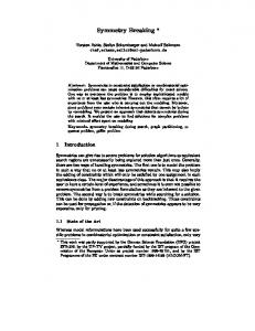
The Match procedure given in Figure 4 is a generalized version of one iteration of the Israeli-Itai [17] matching algorithm. It is given not-necessarily-disjoint node sets U1 , U2 and a matching M , and returns a matching on U1 × U2 that is node-disjoint from M . It works as follows. Each unmatched node in U1 proposes to an unmatched neighbor in U2 , selected uniformly at random. Each node in U2 receiving a proposal accepts one, breaking ties by node ID. The accepted proposals form a set of directed paths and cycles. At this point each node v generates a bit b(v): 0 if v is at the beginning of a path, 1 if at the end of a path, and uniformly at random otherwise. A directed edge (u, v) enters the matching if and only if b(u) = 0 and b(v) = 1. Refer to Figure 5 for an execution of Match on a small graph. The procedure MaximalMatching has a two-phase structure. Phase I consists of O(log ∆) stages in which the matching, M , is supplemented using two calls to Match. After Phase I all components of unmatched vertices have fewer than s = (c ln n)9 nodes, with probability 1 − n−Ω(c) . We

20

Match(U1 , U2 , M ) 1. Each u ∈ U1 \V (M ) proposes to prop(u): prop(u) ← a random neighbor of u in U2 \V (M ). 2. Each v ∈ U2 \V (M ) with a proposal accepts the best one: prop? (v) ← arg max {ID(u)}. u : prop(u)=v

{(prop? (v), v)

3. F ← | v ∈ U2 for which prop? (v) exists} (F is a set of directed edges. It consists of directed paths and cycles.) 4. Each v ∈ U1 ∪ U2 with degF (v) > 0   0 1 b(v) ←  a random value in {0, 1}

chooses a b(v) ∈ {0, 1}: if indegF (v) = 0, if outdegF (v) = 0, otherwise.

5. Return the matching {(u, v) ∈ F | b(u) = 0 and b(v) = 1}. Figure 4:

(a)

(b)

(c)

Figure 5: One possible execution of Match(V, V, ∅). Left: the undirected input graph G = (V, E). Middle: the directed pseudoforest (V, {(u, prop(u))}) induced by the proposals. Right: F consists of directed paths and cycles. The beginning and end of each path are labeled 0 and 1, respectively. Grayed, isolated nodes receive no label. All other nodes are assigned random labels in {0, 1}.

21

apply the deterministic O(log4 s) = O(log4 log n) time maximal matching algorithm of [16] on each component, in parallel. In total the running time is O(log ∆ + log4 log n). def

Let Vi = V (G)\V (M ) be the set of unmatched nodes just before stage i. For brevity we let degi and Γi be the degree and neighborhood functions for the graph induced by Vi . The parameters for stage i are given below. Roughly speaking, δi is the maximum degree at stage i, τi = 2δi /(c ln n) is a certain ‘low-degree’ threshold, and νi = δi τi /2 is a bound on the sum of degrees of nodes in Γi (v), for any v. Define √ def ∆ c ln n δi = , ρi def

τi =

def

and νi =

2∆ √ , ρi c ln n ∆2 δi τi = , 2i ρ 2

def

where ρ =

p 16/15 < 1.033.

Define the low degree and high degree nodes before stage i to be def

Vilo = {v ∈ Vi | degi (v) ≤ τi+1 } def

and Vihi = {v ∈ Vi | degi (v) > δi+1 }. Note that nodes with degree between τi+1 and δi+1 are in neither set. In stage i we supplement the current matching, first with a matching on Vilo × Vihi , then with a matching on Vi . As we soon show, certain invariants will hold after stage i with probability 1 − exp(−Ω(τi )). Thus, in order to obtain high probability bounds we must switch to a different analysis when τi = Θ(log n), that is, when the maximum degree is δi = Θ(log2 n). The algorithm always returns a matching. If, at the beginning of Phase II, C contains all connected components on Vz then the returned matching is clearly maximal. Thus, our goal is to show that with high probability, after Phase I there is no connected component of unmatched P 9 nodes with size greater than (c ln n) . In the lemma below deg(S) is short for u∈S deg(u), where S ⊂V. Lemma 4.1 Define i? to be the last stage for which τi? ≥ 2c ln n. With probability 1 − 2n−c/660+1 , the following bounds hold for all v ∈ V (G) after each stage i < i? . degi+1 (v) ≤ δi+1 (2)

and degi+1 (v) ≤ νi+1 , (2)

def

where degi+1 (v) = degi+1 (Γi+1 (v)). Proof: The inequalities hold trivially when i = 0. We analyze the probability that they hold after stage i, assuming they hold just before stage i. For the sake of minimizing notation we use degi , Γi , etc. to refer to the degree and neighborhood functions just before each call to Match in stage i. This should not cause confusion. (2) Consider a node v ∈ Vi at the beginning of stage i. By assumption degi (v) ≤ δi and degi (v) ≤ νi . Since, by definition, nodes in Vilo have degree at most τi+1 , v has less than νi /τi+1 = δi+1 ·(ρ2 /2) 22

MaximalMatching(Graph G) Phase I: 1. Initialize M0 ← ∅ def

2. For each stage i from 0 to z = logρ ∆+log4/3 (c ln n)−1. M ← M ∪ Match(Vilo , Vihi , M ) M ← M ∪ Match(Vi , Vi , M ) Phase II: Let C be the connected components in the graph induced by Vz containing less than (c ln n)9 nodes. 3. For each C ∈ C , MC ← a maximal matching on C [ 4. Return M ∪ MC . C∈C

Figure 6: neighbors that are not in Vilo . We argue that if v ∈ Vihi (that is, degi (v) > δi+1 ) then v will be matched in the first call to Match in stage i with probability 1 − exp((1 − ρ2 /2)c ln n/2). Note that the forest induced by the proposals consists solely of stars (all edges being directed from Vilo to Vihi ) which implies that F , the graph consisting of accepted proposals, consists solely of single-edge paths. Single-edge paths in F are always committed to the matching since their endpoints’ b-values are chosen deterministically in Step 4 of Match to satisfy the criterion of Step 5. Thus, v ∈ Vihi will be matched if any neighbor u ∈ Vilo chooses (u, v) in Step 2. The probability that this does not occur is at most

1 1− τi

|Γi (v)∩Vilo |

ρ2 1− 2 δi+1 1 ≤ 1− τi ρ2 δi+1 ≤ exp − 1 − 2 τi 2 ρ c ln n = exp − 1 − < n−0.22c 2 2ρ

{ρ < 1.033}

By a union bound, every v ∈ Vihi will be matched with probability more than 1−n−c/5+1 . Therefore, we proceed under the assumption that after the first call to Match in stage i, all unmatched nodes (2) have degree less than δi+1 . It remains to show that after the second call to Match, degi+1 (v) ≤ νi+1 , for all v ∈ V (G). A node v will be guaranteed to have positive degree in F under two circumstances: (i) some node offers v a proposal, or (ii) among those nodes proposing to prop(v), v has the highest ID. Once v is in a path or cycle in F it becomes matched with probability at least 1/2. (It is actually exactly 1/2, except if v is in a single-edge path, in which case it is 1.) 23

Figure 7: The neighborhood of v is partitioned into A and B, and A is partitioned into A0 and A\A0 . Proposals are indicated by directed edges. A node is in A if a majority of its neighbors do not already have a proposal and in B otherwise. An A-node is in A0 if it makes the first proposal to a node. A node is in C if it is adjacent to B and has a proposal. Note: nodes with a proposal that are adjacent to A but not B are not in C. Contrary to the depiction, A-nodes and B-nodes may be adjacent and C may intersect both A and B. ˆ i (v) then expose In the following analysis we first expose the proposals made by all nodes in Vi \Γ ˆ i (v) in descending order of node ID. Consider the moment just before a neighbor the proposals of Γ u ∈ Γi (v) makes a proposal. If at least degi (u)/2 neighbors of u have yet to receive a proposal (by nodes already evaluated) then place u in set A, otherwise place u in set B. If u is put in set A and u does offer prop(u) its first proposal thus far—implying that u will have positive degree in F —then also place u in set A0 . See Figure 7 for an illustration. We split the rest of the analysis into two cases depending on whether A-nodes or B-nodes (2) account for the larger share of edges in v’s 2-neighborhood. In both cases we show that degi+1 (v) ≤ νi+1 with high probability.

4.1

Case I: The A-nodes (2)

(2)

We first analyze the case that degi (A) ≥ degi (v)/2 ≥ νi+1 /2. (If degi (v) is already less than νi+1 there is nothing to prove.) Observe that each node u, once in A, is moved to A0 with probability at least 1/2, and if so, contributes degi (u) ≤ δi+1 to degi (A0 ).14 The probability that after evaluating 14 Note that this process fits in the martingale framework of Corollary A.5. Here Xj is the state of the system after evaluating the jth neighbor u of v and Zj is degi (u) if u joins A0 and 0 otherwise, which is a function of Xj . Thus, each Zj has a range of at most δi+1 .

24

each u ∈ Γi (v), degi (A0 ) is less than a

√1 -fraction 2

Pr(degi (A0 ) < √12 · E[degi (A0 )])   (1 − √12 ) E[degi (A0 )] 2  P ≤ exp− 2 u∈A (degi (u))2   (1 − √12 ) 12 degi (A) 2  ≤ exp− 2 2(degi (A)/δi+1 )δi+1 ! ! (1 − √12 )2 deg (A) i ≤ exp − 8 δi+1 ! ! (1 − √12 )2 ≤ exp − τi+1 32

of its expectation is

{Corollary A.5}

{linearity of expectation}

degi (A) ≥

< n−c/187

νi+1 δi+1 τi+1 = 2 4

{τi+1 ≥ τi? ≥ 2c ln n}

We proceed under the assumption that this unlikely event does not hold, so degi (A0 ) ≥ E[degi

(A0 )]

≥

1 √ 2 2

· degi (A) ≥

1 √ 4 2

√1 2

·

· νi+1 . Since each node with positive degree in F is matched

with probability at least 1/2, by linearity of expectation E[degi (A0 ) − degi+1 (A0 )] ≥ 12 degi (A0 ). Moreover, whether v ∈ A0 is matched depends only on the b-values of neighboring nodes in F . The dependency graph of these events has chromatic number χ = 5 since the nodes of a cycle can be 5-colored such that any two nodes within distance 2 receive different colors. The probability that degi (A0 ) − degi+1 (A0 ) is less than a √12 -fraction of its expectation is therefore Pr degi (A0 ) − degi+1 (A0 ) < √12 · E[degi (A0 ) − degi+1 (A0 )]   2 1 − √12 E[degi (A0 ) − degi+1 (A0 )] 2  P {Theorem A.3, χ = 5} ≤ exp− χ · u∈A0 (degi (u))2   2 1 − √12 12 degi (A0 ) 2  ≤ exp− 2 χ · (degi (A0 )/δi+1 )δi+1 ! ! (1 − √12 )2 deg (A0 ) i ≤ exp − 10 δi+1 ! ! (1 − √12 )2 νi+1 δi+1 τi+1 √ √ τi+1 ≤ exp − degi (A0 ) ≥ √ = 80 2 4 2 8 2 < n−c/660

{τi+1 ≥ τi? ≥ 2c ln n}

25

To sum up, if this unlikely event does not occur, (2)

(2)

degi (v) − degi+1 (v) ≥ degi (A0 ) − degi+1 (A0 ) {because A0 ⊆ Γi (v)} 1 ≥ √ · E[degi (A0 ) − degi+1 (A0 )] 2 1 1 1 (2) 0 √ 2 · degi (A) ≥ ≥ √ · degi (A ) ≥ degi (v). 16 2 2 2 2 (2)

Thus, with high probability, degi+1 (v) ≤

4.2

15 16

(2)

· degi (v).

Case II: The B-nodes (2)

We now turn to the case when degi (B) ≥ 12 · degi (v) ≥ 12 · νi+1 . By definition, just before any u ∈ B makes its proposal, at least 12 · degi (u) of its neighbors have already received a proposal. We do not care who u proposes to. Let C ⊆ Γi (B) be the set of nodes in B’s neighborhood that receive at least one proposal. For x ∈ C, let degB (x) ≤ δi+1 be the number of its neighbors in B. Thus, if x is matched then deg(2) (v) is reduced by at least degB (x). It follows that X X X1 degB (x) = degC (u) ≥ degB (C) = {by defn. of u ∈ B} · degi (u) 2 x∈C

u∈B

u∈B

1 1 1 (2) = · degi (B) ≥ · degi (v) > · νi+1 . 2 4 4 Since C-nodes are matched with probability 1/2, by linearity of expectation, E[degi+1 (B)] ≤ degi (B) − 12 · degB (C) ≤ 34 degi (B). We bound the probability that degi+1 (B) deviates from its expectation using Janson’s inequality, in exactly the same way as we bounded degi+1 (A0 ). It follows that 1 Pr degi+1 (B) ≥ degi (B) − · degB (C) 4 ! 2( 14 degB (C))2 ≤ exp − P {Theorem A.3} χ · x∈C (degB (x))2 1 (degB (C))2 {χ = 5, degB (x) ≤ δi+1 } ≤ exp − · 2 40 (degB (C)/δi+1 )δi+1 1 ≤ exp − τi+1 {degB (C) ≥ νi+1 /4 = δi+1 τi+1 /8} 320 ≤ n−c/160

{τi+1 ≥ τi? ≥ 2c ln n}

Thus, with high probability (2)

(2)

degi+1 (v) ≤ degi (v) −

1 15 (2) · degB (C) ≤ · degi (v), 4 16

(2)

(2)

(2)

15 since degB (C) ≥ 41 ·degi (v). Whether we are in Case I or Case II, degi+1 (v) ≤ 15 16 ·degi (v) ≤ 16 ·νi p with high probability. Since νi+1 = νi /ρ2 , we set ρ = 16/15. By a union bound, the probability of error at any node is at most 2n−c/660+1 . This covers the probability that the first call to Match fails to match all Vihi -nodes or the second call fails to make (2) degi+1 (v) ≤ νi+1 , for all v ∈ Vi .

26

4.3

The Emergence of Small Components

Lemma 4.1 implies that before stage i? < logρ ∆, the maximum degree is at most δi? = τi? (c/2) ln n ≤ (c ln n)2 . In Lemmas 4.2 and 4.3 we prove that after another O(log log n) iterations of the Match procedure, all components of unmatched vertices have size at most (c ln n)9 , with high probability. Thus, Phase II of MaximalMatching correctly extends the matching after Phase I to a maximal matching. Lemma 4.2 For any node v and any stage i, Pr degi+1 (v) ≤

3 4

· degi (v) ≥ 14 .

Proof: We analyze the expected drop in v’s degree during the second call to Match (the one in which all nodes participate), then apply Markov’s inequality. Expose the proposals in descending order of node ID, and consider the moment just before v makes its proposal. Let P ⊆ Γi (v) be those neighbors already holding a proposal and Q ⊆ Γi (v) be the neighbors with no proposal. All nodes in P will be matched with 1/2 probability and v will be matched with 1/2 probability if it proposes to a member of Q. The probability v is matched is at least 2 , where = |Q|/ degi (v). The probability that u ∈ P is still a neighbor of v after this call to Match is therefore at most 12 (1 − 2 ). The probability that u ∈ Q is still a neighbor is at most 1 − 2 . By linearity of expectation, E[degi+1 (v)] ≤ 1 − 2 + 12 (1 − ) 1 − 2 · degi (v) = (1 − 2 )( 12 + 2 ) · degi (v) ≤ ( 43 )2 · degi (v)

{maximized at = 1/2}

7 That is, we lose at least a 16 -fraction of v’s neighbors in expectation. By Markov’s inequality, 3 Pr degi+1 (v) ≤ 4 · degi (v) ≥ 41 .

ˆ be the subgraph induced by unmatched nodes at some point in Phase I, whose Lemma 4.3 Let G ˆ After 12 log4/3 ∆ ˆ more stages in Phase I, all components of unmaximum degree is at most ∆. ˆ 4 with probability 1 − n−c , where t def matched nodes have size at most t∆ = c ln n. Proof: The proof follows the same lines at that of Lemma 3.2 and 3.3, but has some added ˆ complications. We say v is successful in stage i if degi+1 (v) ≤ 34 · degi (v). If v experiences log4/3 ∆ successes then either v has been matched or all neighbors of v are matched. The events that u and v are successful in a particular stage i are independent if distGˆ (u, v) ≥ 5 since the success of u and v only depend on the random choices of nodes within distance 2. Any ˆ 4 must contain a subset T of t nodes such that (i) each pair of nodes in T is at subgraph of size t∆ ˆ 5 . Call T a distance-5 set if |T | = t and it distance at least 5 and (ii) T forms a t-node tree in G t 5(t−1) ˆ ˆ (There are less than satisfies (i) and (ii). There are less than 4 · n · ∆ distance-5 sets in G. t 5(t−1) ˆ 4 topologically distinct trees with t nodes and less than n∆ ways to embed one such tree in ˆ 5 .) G ˆ consecutive stages, v ∈ T experiences some Consider any distance-5 set T . Over 12 log4/3 ∆ def P number of successful stages. Call this random variable Xv and define X = v∈T Xv . By Lemma 4.2 and linearity of expectation, X ˆ = 3t log4/3 ∆. ˆ E[X] = E[Xv ] ≥ t · 41 (12 log4/3 ∆) v∈T

27

ˆ then some Xv ≥ log4/3 ∆, ˆ implying that v becomes isolated and therefore that no If X ≥ t log4/3 ∆ component contains all T -nodes. We will call T successful if any member of T becomes isolated. By a Chernoff bound (Theorem A.2), the probability that T is unsuccessful is at most 1 ˆ Pr X < t log4/3 ∆ ≤ Pr X < · E[X] 3 ! 2 23 E[X] 2 ≤ exp − ˆ 4t log4/3 ∆ ˆ ˆ ≤ exp −2t log4/3 ∆ {E[X] ≥ 3t log4/3 ∆} ˆ −(2 log4/3 e)t =∆ ˆ stages, if there exists a component with size t∆ ˆ 4 then it must contain an unsucAfter 12 log4/3 ∆ cessful subset T . By the union bound, this occurs with probability less than ˆ 5(t−1) · ∆ ˆ −(2 log4/3 e)t 4t · n · ∆ ˆ (5−2 log4/3 e)·c ln n < 4c ln n · n · ∆ < n−c

ˆ sufficiently large. Note: 5 − 2 log4/3 e < 0.} {for ∆

Theorem 4.4 In a graph with maximum degree ∆, a maximal matching can be computed in O(log ∆ + log4 log n) time with high probability using O(1)-size messages. When the graph is bipartite and 2-colored, the time bound becomes O(log ∆ + log3 log n). ˆ = (c ln n)2 , with Proof: After i? = logρ (∆/(c ln n)3/2 ) stages in Phase I the maximum degree is ∆ ˆ stages in Phase I all connected components have at most high probability. After another 4 log4/3 ∆ def ˆ 4 s = ∆ · c ln n = (c ln n)9 nodes, with high probability. We execute the deterministic maximal matching algorithm of [16] for time sufficient to solve any instance on s nodes: O(log4 s) time for general graphs and O(log3 s) time for bipartite, 2-colored graphs. Both Phase I and Phase II can be implemented with O(1)-size messages, that is, this algorithm works in the CONGEST model.

5

Vertex Coloring

We consider a slightly more stringent version of (∆ + 1)-coloring called (deg +1)-coloring, where each node v must adopt a color from the palette {1, . . . , deg(v) + 1}, or more generally, an arbitrary set with size deg(v) + 1.15 Although the palette of a node does not depend on ∆, our algorithm still requires that nodes know ∆ and n. In Section 5.1 we define and analyze a natural O(1)-time algorithm called OneShotColoring that colors a subset of the nodes. Johannson [18] showed that O(log n) applications of a variant of OneShotColoring suffice to (∆ + 1)-color a graph, with high probability. Our goal is to show something stronger. We show that after O(log ∆) applications of OneShotColoring, all nodes have at most O(log n) uncolored neighbors that each have Ω(log n) uncolored neighbors. This property 15

Some applications [3] demand (deg +1)-colorings, not (∆ + 1)-colorings.

28

OneShotColoring(G, Color) Define U ⊆ V (G) and Ψ : V (G) → 2{1,...,∆+1} as follows. def

U = {u ∈ V (G) | Color(u) = ⊥}, def

and Ψ(v) = {1, . . . , deg(v) + 1}\ Color(Γ(v)),

the uncolored vertices, v’s available palette.

The following steps are executed for all v ∈ U , in parallel. 1. Select a Color? (v) ∈ Ψ(v) uniformly at random. 2. If ID(v) > max {ID(u) | u ∈ ΓU (v) and Color? (u) = Color? (v)}, Permanently assign Color(v) ← Color? (v). Figure 8: allows us to reduce the resulting (deg +1)-coloring problem to two (deg +1)-coloring problems on subgraphs with maximum degree O(log n). It is shown that on these instances, O(log log n) further applications of OneShotColoring suffice to reduce the size of all uncolored components to poly(log n). In Phase II we apply the deterministic (deg +1)-coloring algorithm of Panconesi and Srinivasan [32] to the poly(log n)-size uncolored components. The remainder of this section constitutes a proof of Theorem 5.1. Theorem √ 5.1 In a graph with maximum degree ∆, a (deg +1)-coloring can be computed in O(log ∆+ exp(O( log log n))) time using poly(log n)-length messages.

5.1

Analysis of OneShotColoring

The algorithm maintains a proper partial coloring Color : V (G) → {1, . . . , ∆ + 1, ⊥}, where ⊥ denotes no color and Color(v) ∈ {1, . . . , deg(v) + 1} ∪ {⊥}. Initially Color(v) ← ⊥ for all v ∈ V (G). Before a call to OneShotColoring some nodes have already committed to their final colors. Each remaining uncolored node v chooses Color? (v), a color selected uniformly at random from its remaining palette. It may be that neighbors of v also choose Color? (v). If v holds the highest ID among all such nodes contending for Color? (v), it permanently commits to that color. The pseudocode for OneShotColoring appears in Figure 8. We analyze the properties of OneShotColoring from the point of view of some arbitrary uncolored node v ∈ U . Note that whether v is colored depends only on its behavior and the behavior of def def −1 neighbors with larger IDs, denoted Γ> U (v) = {u ∈ ΓU (v) | ID(u) > ID(v)}. Define Ψ (q) = {u ∈ Γ> of v’s uncolored neighbors that are contending for color U (v) | q ∈ Ψ(u)} to be the set P q and have higher IDs. Define w(q) = u∈Ψ−1 (q) 1/|Ψ(u)| to be the weight of color q. In other words, each neighbor u distributes 1/|Ψ(u)| units of weight to each color in its palette. Note that 1/|Ψ(u)| ≤ 1/(degU (u) + 1) ≤ 1/2. The probability that q ∈ Ψ(v) is available to v after exposing

29

Color? (Γ> U (v)) is Y

Pr(q 6∈ Color? (Γ> U (v))) =

1−

1 |Ψ(u)|

u∈Ψ−1 (q)

Y

≥

1 1/|Ψ(u)| 4

(1)

u∈Ψ−1 (q)

=

1 w(q) . 4

Inequality (1) follows from the fact that (1 − x) ≥ (1/4)x whenPx ∈ [0, 1/2]. Let Xq ∈ {0, 1} be the indicator variable for the event that q is available and X = q Xq . By linearity of expectation, P E[X] ≥ q∈Ψ(v) 41 w(q) . By the convexity of the exponential function, this quantity is minimized when all color weights are equal. Hence, E[X] ≥

X

1 w(q) 4

P

w(q)/|Ψ(v)|

≥ |Ψ(v)| ·

1 4

≥ |Ψ(v)| ·

1 degU (v)/|Ψ(v)| 4

q

q∈Ψ(v)

> |Ψ(v)|/4.

(2) (3)

Inequalities (2,3) follow from the fact that each neighbor in Γ> U (v) can contribute at most one unit (v) + 1. We will call v happy if X ≥ |Ψ(v)|/8, that of weight and that |Ψ(v)| ≥ degU (v) + 1 ≥ deg> U is, if the number of available colors is at least half its expectation. Let Hv be the event that v is happy. The variables {Xq } are not independent. However, Dubhashi and Ranjan [13] showed that {Xq } are negatively correlated, and more generally that all balls and bins experiments of this form give rise to negatively correlated variables.16 By Theorem A.2, |Ψ(v)| 2 · (|Ψ(v)|/8)2 |Ψ(v)| def Pr(Hv ) = Pr X < < exp − = exp − . 8 |Ψ(v)| 32 Lemma 5.2 summarizes the relevant properties of OneShotColoring used in the next section. Lemma 5.2 Let U be the uncolored nodes before a call to OneShotColoring and v ∈ U be arbitrary. 1. Pr(v is colored) > 1/4. (v)+1 2. Pr(Hv ) > 1 − exp − degU32 .

5.2

A (deg +1)-Coloring Algorithm

It goes without saying that our (deg +1)-Coloring algorithm (Figure 9) has a two-phase structure. The ultimate goal of Phase I is to reduce the global problem to some number of independent (deg +1)-coloring subproblems, each on poly(log n)-size components, which can be colored deterministically in Phase II. We first prove that this is possible with O(log log n) applications of OneShotColoring, if the uncolored subgraph already has maximum degree poly(log n). 16

In this situation the colors are bins and the neighbors’ choices are balls.

30

ˆ be the maximum degree Lemma 5.3 Apply an arbitrary proper partial coloring to G, and let ∆ ˆ in the subgraph induced by uncolored nodes. After 5 log4/3 ∆ iterations of OneShotColoring, all ˆ 2 nodes with probability 1 − n−c , where t def uncolored components have less than t∆ = c log ˆ n. ∆

Proof: The proof is similar to that of Lemma 3.3 and Lemma 4.3. Whether a node is colored depends only on the color choices of nodes in its inclusive neighborhood. Thus, if two nodes are at distance at least 3, their coloring events are independent. Let T ⊂ U be a distance-3 set, that is, one for which (i) |T | = t = c log∆ ˆ n, (ii) the distance between each pair of nodes is at least 3, and ˆ 3(t−1) < n4c distance-3 (iii) T forms a tree in the uncolored part of G3 . There are less than 4t · n · ∆ ˆ sets and the probability that one is entirely uncolored after 5 log4/3 ∆ iterations of OneShotColoring is, by Lemma 5.2, less than ˆ 3 5t log4/3 ∆ 4

=

ˆ 3 5(c log∆ ˆ n) log4/3 ∆ 4

= n−5c .

By a union bound, no distance-3 set exists with probability n4c−5c = n−c . Moreover, if there were ˆ 2 after 5 log4/3 ∆ ˆ iterations of OneShotColoring, it would have an uncolored component with size t∆ to contain such a distance-3 set. p Lemma 5.3 implies a (deg +1)-coloring algorithm running in O(log ∆+exp(O( log(∆2 log n)))) time. Once the component size is less than ∆2 log n we can apply the deterministic (deg +1)coloring algorithm √ of Panconesi and Srinivasan [32] to each uncolored component. The exponential dependence on log ∆ is undesirable. Using Lemma 5.2 we show that, roughly speaking, degrees decay geometrically with each call to OneShotColoring, with high probability. This will allow us to √ reduce the dependence on n to exp(O( log log n)). ˆ to be those high degree uncolored nodes, Lemma 5.4 Define U hi = {u ∈ U | degU (u) > ∆} def ˆ = c ln n. Let U0 and U1 be the uncolored nodes before and after a particular call to where ∆ def T OneShotColoring. Let H = v∈U hi Hv be the event that all U0hi nodes are happy. 0

1. Pr(H ) < n−c/32+1 . 2. Pr degU hi (v) ≤ 15 · deg (v) > 1 − n−c/512 − n−c/32+1 . hi U 16 1

0

ˆ = c ln n, and the union bound, Proof: By Lemma 5.2(2), the definition of ∆ ! ˆ +1 ∆ hi Pr(H ) < |U0 | · exp − < n−c/32+1 . 32 In other words, with high probability, every vertex in U0hi has a 1/8 fraction of its palette available to it. Turning to Part 2, fix any vertex v ∈ U0hi . There are two ways a neighbor of v in U0hi can fail to be a neighbor in U1hi after this call to OneShotColoring. It can either be colored (in which case it is not in U1 ) or a sufficient number of its neighbors can be colored so that it is no longer in U1hi . We ignore the second possibility and analyze the number of neighbors of v in U0hi that are colored. List the nodes of ΓU hi (v) in decreasing order of ID as u1 , . . . , udeg hi (v) . At step 0 we expose Color? (u) 0

U0

for all u 6∈ ΓU hi (v) and at step i we expose Color? (ui ). Let Yi be the information exposed after 0

31

step i. Whether ui is successfully colored is a function of Yi . Moreover, the probability that ui is colored, given Yi−1 , is precisely the fraction of its palette that is still available, according to Yi−1 . P Let Xi ∈ {0, 1} be the indicator variable for the event that ui is colored and X = i Xi . Unless the unlikely event H occurs, Pr(Xi = 1 | Yi−1 ) = Pr(ui is colored | Yi−1 ) ≥ 1/8, and by Corollary A.5, Pr(X
∆

uncolored nodes high-degree nodes

Ghi ← the graph induced by U hi Glo ← the graph induced by U \U hi ˆ times: 4. Repeat 5 log4/3 ∆ OneShotColoring(Ghi , Color) ˆ times: 5. Repeat 5 log4/3 ∆ OneShotColoring(Glo , Color) Phase II: ˆ 3. 6. Color all remaining uncolored components of Ghi with size at most ∆ ˆ 3. 7. Color all remaining uncolored components of Glo with size at most ∆ Figure 9:

33

Sparsify(Graph G, Integer f ) 1. Initialize U ← ∅. 2. For i from 1 to logf ∆, ˆ ), independently, and in parallel: (a) For each v ∈ V (G)\Γ(U Set U ← U ∪ {v} with probability (c ln n)f i /∆. 3. Return U . (2, β)-RulingSet(Graph G) 1. R0 ← V (G) 2. For i from 1 to β − 1 Ri ← Sparsify(Gi−1 , fi ), where Gi−1 is the graph induced by Ri−1 . 3. Rβ ← MIS(Gβ−1 ) 4. Return(Rβ ) Figure 10: The algorithm for computing Ri from Ri−1 (which satisfies Properties (i) and (ii)) was first described by Kothapalli and Pemmaraju [21]. For the sake of completeness we reproduce this sparsification algorithm and its analysis. Refer to Figure 10 for the pseudocode of Sparsify and (2, β)-RulingSet. Lemma 6.1 (Kothapalli and Pemmaraju [21]) Given G = (V, E) and a threshold f , a subset U ⊆ V can be computed in O(logf ∆) time such that for every v ∈ V (G), distG (v, U ) ≤ 1, and for every v ∈ U , degU (v) ≤ 2cf ln n, with probability n−c+2 . Proof: Consider an execution of Sparsify(G, f ). Let Ui be U after the ith iteration of the loop and def ˆ i ). Assume, inductively, that just before the ith iteration the maximum degrees in the Vi = V \Γ(U graphs induced by Vi−1 and Ui−1 are at most ∆/f i−1 and f · 2c ln n. These bounds hold trivially when i = 1. Each v ∈ Vi−1 is included in Ui independently with probability c ln nf i /∆, so the ˆ i ) is less than (1−c ln nf i /∆)∆/f i < probability that a v ∈ Vi−1 with degVi−1 (v) > ∆/f i is not in Γ(U n−c . Furthermore, if v ∈ Ui , E[degUi (v)] = degVi−1 (v) · c ln nf i /∆ ≤ cf ln n. By Theorem A.1, the probability that degUi (v) ≥ 2cf ln n is at most exp(−f c ln n/3) < n−c . Note that since v and its neighborhood are permanently removed from consideration, it never acquires new neighbors in U , so degUi (v) = degU (v). Thus, with high probability the induction hypothesis holds for the next iteration. 1 √ Theorem 6.2 A (2, β)-ruling set can be computed in O(β log β−1/2 ∆ + exp(O( log log n))) time with high probability. 34

Proof: The algorithm simply consists of β − 1 calls to Sparsify followed by a call to MIS. Every node in Ri−1 is in or adjacent to Ri , for 1 ≤ i < β, which implies that dist(v, Rβ ) ≤ β for all v ∈ V . Since Rβ is an independent set it is also a (2, β)-ruling set. The time to compute Rβ is on the order of p log(fβ−2 log n) log ∆ log(f1 log n) + + ··· + + log2 (fβ−1 log n) + exp(O( log log n)). log f1 log f2 log fβ−1 1−i(

2

2

)

2β−1 , the time for each call to Sparsify is O((log ∆) 2β−1 ) and the time Setting log fi = (log ∆) √ for the final MIS is exp(O( log log n)) plus

2

log fβ−1 = (log ∆)

2 2 1−(β−1) 2β−1

2

= (log ∆) 2β−1 .

Theorem 6.2 highlights an intriguing open problem. Together with the KMW lower bound, it shows that (2, 2)-ruling sets are provably easier √ to compute than (2, 1)-ruling sets, the upper 2/3 bound for the former being O(log ∆ + exp(O( log log n))) and the lower bound on the latter being Ω(log ∆). Is it possible to obtain any non-trivial lower bound on the complexity of computing (2, β)-ruling sets for some β > 1? In order to apply [24] one would need to invent a reduction from O(1)-approximate minimum vertex cover to (2, β)-ruling sets.

7

Bounded Arboricity Graphs

Recall that a graph has arboricity λ if its edge set is the union of λ forests. In the proofs of Lemma 7.1 and Theorem 7.2, degE 0 (u) is the number of edges incident to u in E 0 ⊆ E and degV 0 (u) is the number of neighbors of u in V 0 ⊆ V . Lemma 7.1 Let G be a graph of m edges, n nodes, and arboricity λ. 1. m < λn. 2. The number of nodes with degree at least t ≥ λ + 1 is less than λn/(t − λ). 3. The number of edges whose endpoints both have degree at least t ≥ λ+1 is less than λm/(t−λ).

Proof: Part 1 follows from the definition of arboricity. For Parts 2 and 3, let U = {v | degG (v) ≥ t} be the set of high-degree nodes. We have that λn > m ≥ |{(u, v) ∈ E(G) | u ∈ U or v ∈ U or both}| X 1X ≥ (t − degU (u)) + degU (u) 2 u∈U

u∈U

≥ t · |U | − |E(U )| > (t − λ) · |U |. Thus |U | < λn/(t − λ), proving Part 2. Part 3 follows since the number of such edges is less than λ|U | ≤ λm/(t − λ).

35

Theorem 7.2 Let G be a graph of arboricity λ and maximum degree ∆, and let t ≥ max{(5λ)8 , (4(c+ 1) ln n)7 } be a parameter. In O(logt ∆) time we can find a matching M ⊆ E(G) (or an independent set I ⊆ V (G)) such that with probability at least 1 − n−c , the maximum degree in the graph induced ˆ by V \V (M ) (or the graph induced by V \Γ(I))) is at most tλ. Proof: In O(logt n) rounds we commit edges to M (or nodes to I) and remove all incident edges (or incident nodes). Let G be the graph still under consideration before some round and let H = {v ∈ V | degG (v) ≥ tλ} be the remaining high-degree nodes. Our goal is to reduce the size of H by a roughly t1/7 factor. Let J = {v ∈ H | degH (v) ≥ tλ/2}. It follows that any node def ˜ be v ∈ H0 = H\J has degV \H (v) ≥ tλ/2 since at most tλ/2 of its neighbors can be in H. Let E 0 any set of edges crossing the cut (H, V \H) such that for v ∈ H , degE˜ (v) = tλ/2. In other words, ˜ discard all but tλ/2 edges incident to each H0 node arbitrarily. Let S = {u | v ∈ H0 and (v, u) ∈ E} ˜ Note that |S| ≤ tλ|H0 |/2. See Figure 11. We define be the neighborhood of H0 with respect to E.

...

..

.

...

Figure 11: Good S-nodes have fewer than β neighbors in H0 and fewer than β 2 neighbors in S. Good H0 -nodes have at least tλ/4 good neighbors in S. ˜ bad S-nodes, bad E-edges, and bad H0 -nodes as follows, where β = t1/7 . BS = u ∈ S | degE˜ (u) ≥ β or degS (u) ≥ β 2 or both , n o ˜ u ∈ BS , BE˜ = (u, v) ∈ E n o and BH0 = v ∈ H0 degBE˜ (v) > λt/4 . By Lemma 7.1(3) the number of edges (u, v) ∈ BE˜ designated bad because degE˜ (u) ≥ β is less ˜ than λ|E|/(β − λ). By Lemma 7.1(2) the number of additional edges (u, v) ∈ BE˜ designated bad because degS (u) ≥ β 2 is at most (β − 1)λ|S|/(β 2 − λ) since there are less than λ|S|/(β 2 − λ) such

36

˜ In total we have nodes and each contributes fewer than β edges to E. ˜ λ|E| (β − 1)λ|S| + β−λ β2 − λ λ(tλ|H0 |/2) (β − 1)λ(tλ|H0 |/2) ≤ + β−λ β2 − λ β−1 1 2 0 + = λ t|H | 2(β − λ) 2(β 2 − λ) λ2 t|H0 | < . β−λ

|BE˜ |
0. A graph of maximum degree ∆ and arboricity λ can, with high probability, be (∆ + λ1+ )-colored in O(log ∆ + log λ log log n) time or (∆ + O(λ))-colored in O(log ∆ + min{λ log log n, λ + (log log n)1+ }) time. Furthermore, a (deg +1)-coloring can, with high probability, be computed in time on the order of   log ∆ + λ + λ log log n,       1+ log ∆ + λ + (log log n) , min .     log ∆ + λ1+ + log λ log log n  Proof: Following the algorithm from Section 5, we first execute O(log ∆) iterations of OneShotColoring ˆ def then decompose the problem into two subproblems on a graph with maximum degree ∆ = Θ(log n). ˆ On each subproblem we perform another O(log ∆) iterations of OneShotColoring, after which the subgraph induced by uncolored nodes consists, with high probability, of components with size at ˆ 2 log ˆ n = o(log3 n). At this point we apply one of the deterministic Barenboim-Elkin [6] most s = ∆ ∆ coloring algorithms to each such component using a fresh palette of p previously unused colors, say {−1, . . . , −p}. We can find a p-coloring with p = λ1+ in O(log λ log s) = O(log λ log log n) time or with p = O(λ) in O(min{λ log s, λ + (log s)1+ }) = O(min{λ log log n, λ + (log log n)1+ }) time. Every v ∈ V (G) has been assigned a color Color(v) ∈ {1, . . . , deg(v) + 1} ∪ {−1, . . . , −p}. To obtain a (deg +1)-coloring we examine each color κ ∈ {−1, . . . , −p} in turn, letting every node v with Color(v) = κ recolor itself using an available color from {1, . . . , deg(v) + 1}. Theorem√7.6 ([5] + [4]) A (2, O(log λ + O(log λ + log n) time.

√

log n))-ruling set can be computed deterministically in √

Proof: Begin by computing a decomposition of the edge set into λ √ · 2 log n oriented forests, in √ 2 2 O( log n) time [5, §3]. Given this decomposition, compute an O(λ √ · 2 log n )-coloring, in O(log∗ n) time [5, §5.1.2]. Finally, using this coloring, compute a (2, O(log λ + log n))-ruling set in O(log λ + √ log n) time [4].

7.2

Maximal Matching in Trees

√ Our maximal matching √ algorithm from Theorem 7.3 runs in O( log n) time for every arboricity λ from 1 (trees) to 2O( log n) . We argue that this bound is optimal even for λ = 1 by appealing to the KMW lower bound [23, 24]. In [24] it is shown that there exist constants 0 < 3c < c0 such that any (possibly randomized) algorithm minimum vertex cover (MVC) in √ for computing an approximate √ graphs with girth at least c0 · log n either (i) runs in c log n time, or (ii) has approximation ratio 17

The leading constant in the palette size is exponential in 1/.

39

ω(1). We review below √ a well known reduction from 2-approximate MVC to maximal matching, which implies an Ω( log n) lower bound for maximal matching algorithms √ that succeed with high probability. √The graphs used in the KMW bound have arboricity 2O( log n) , so it does directly imply an Ω( log n) lower bound on trees. −2 Theorem 7.7 For some absolute constant√c > 0, no algorithm can, with √ probability 1 − n , compute a maximal matching on a tree in c log n time, nor in c log ∆ + o( log n) time for every ∆.

Proof: We first recount the lower bound for maximal matching on general graphs. Suppose, for the purpose of√ obtaining a contradiction, that there exists a maximal matching algorithm running in time c log n on the KWM graph that fails with probability at most √ 1/n. To obtain an approximate MVC algorithm, run the maximal matching algorithm for c log n time. Any matched node joins the approximate MVC, as well as any node that detects a local violation, namely a node incident to another unmatched node. As the MVC is at least the size of any maximal matching, the expected approximation ratio of this algorithm is at most 2 · Pr(no failure occurs) + n · Pr(some failure occurs) ≤ 2 + n · n1 = 3, a contradiction. Hence there is no algorithm that runs √ √ for c · log n time in graphs with girth at least c0 · log n that computes a maximal matching with probability at least 1 − 1/n. √ We use an indistinguishability argument to show that the Ω( log n) lower bound also holds for trees, and therefore any class of graphs that includes trees. Observe that to show a lower bound for a randomized algorithm, it is enough to prove the same lower bound under the assumption that the identities of graph nodes were selected independently and uniformly at random, from, say, [1, n10 ]. Suppose there is, in fact, an algorithm that given a tree with √ a random (in the above sense) assignment of identities, constructs a maximal matching within c · log n time with success √ −2 . Run this algorithm for c · probability at least 1 − n log n time on the KMW graph G with √ 0 girth c · log n, assuming random assignment of identities in G. Due to the girth bound, the view of every node in G is identical to its view in a tree, and thus from its perspective a correct maximal matching must be computed with probability at least 1−n−2 . By a union bound, a correct maximal −1 matching for the entire graph G will be computed with √ probability at least 1 − n , a contradiction. Θ( log n) and girth Θ(log ∆). All the KMW-based √ √The KMW graph has maximum degree ∆ = 2 Ω( log n) lower bounds can be scaled down to Ω(log ∆) lower bounds (for any ∆ < 2O( log n) ) simply by applying the lower bound argument to the union of numerous identical KMW graphs. Remark 7.8 Theorem 7.7 posited the existence of a maximal matching algorithm for trees whose global probability of failure is n−2 . When we run this algorithm on the KMW graph we can no longer use n−2 as√the global failure probability. It may be that, when run in an actual tree, nodes within distance c log n of a leaf node fail with probability zero: all the failure probability is concentrated at the small set of nodes that cannot “see” the leaves. In the KMW graph all nodes think they are in this small set. We must assume, pessimistically, that failure occurs at every node in the KMW graph with probability n−2 . Remark 7.9 Theorem 7.7, strangely, does not imply any lower bound for the MIS problem on trees, even √ though MIS appears to be just as hard as maximal matching on any class of graphs. The Ω( log n) lower bound for MIS √ [23, 24] is obtained by considering the line graph of the KWM graph, which has girth 3, not Θ( log n). Thus, our indistinguishability argument does not apply. 40

8

MIS in Trees and High Girth Graphs

One of the MIS algorithms of Luby [29] works as follows. In each round each remaining node v chooses a random real r(v) ∈ (0, 1) and includes itself in the MIS if r(v) is greater than maxw∈Γ(v) r(w), thereby eliminating v and its neighborhood from further consideration.18 Observe that the probability that v joins the MIS in a round is 1/(deg(v) + 1), irrespective of the degrees of its neighbors. We would like to say that degrees decay geometrically, that is, after O(k) iterations of Luby’s algorithm the maximum degree is ∆/2k , with high probability. Invariant 8.1 is not quite this strong but just as useful, algorithmically. It states that after O(k log log ∆) iterations, no node has ∆/2k+2 neighbors with degree at least ∆/2k , provided that ∆/2k is not too small. Invariant 8.1 At the end of scale k, for all v ∈ VIB , n o w ∈ ΓIB (v) | degIB (w) > ∆/2k ≤ max{∆/2k+2 , 12 ln ∆}. Randomness plays no role in Invariant 8.1: it holds with probability 1. Any node that violates the invariant is marked bad (placed in B) and temporarily excluded from consideration. As we will soon prove, the probability a node is marked bad is 1/poly(∆). We will only make use of Invariant 8.1 when ∆/2k+2 is, in fact, greater than 12 ln ∆, so the 12 ln ∆ term will not be mentioned until we need to have a lower bound on ∆/2k+2 . Lemma 8.2 In one iteration of scale k, a node w with degIB (w) > ∆/2k is eliminated (appears ˆ in Γ(I)) with probability at least (1 − o(1))(1 − e−1/4 ) > 0.22. Moreover, this probability holds even if we condition on arbitrary behavior at a single neighbor of w. Proof: By Invariant 8.1, |{x ∈ ΓIB (w) | degIB (x) > ∆/2k−1 }| ≤ ∆/2k+1 . Let M be the neighbors of w with degree at most ∆/2k−1 , so |M | ≥ degIB (w) − ∆/2k+1 > ∆/2k+1 . Refer to the portion of Figure 13 depicting w and its neighborhood. The probability that w is eliminated is minimized when M -nodes attain their maximum degree ∆/2k−1 , so in the calculations below we shall assume this is the case. Let x? ∈ M be the first neighbor for which r(x? ) > max{r(y) | y ∈ ΓIB (x? )\{w}}. The probability x? exists is at least Y 1 1 ∆/2k+1 Pr(x? exists) = 1 − 1− ≥1− 1− > 1 − e−1/4 . degIB (x) ∆/2k−1 x∈M

Since, in the most extreme case, degIB (x) = ∆/2k−1 , Pr(x? joins I | x? exists) = Pr(r(x? ) > 1 . The probability that w is eliminated is therefore at least (1 − r(w) | x? exists) ≥ 1 − ∆/2k−1 +1 1 )(1 − e−1/4 ) ∆/2k−1 +1

1 1/4 ) > 0.22 > 1/5. Moreover, this probability is perturbed > (1 − 96 ln ∆ )(1 − e

by a negligible (1 − Θ(1/∆/2k )) = (1 − o(1)) factor if one conditions on arbitrary behavior by a single neighbor of w. Lemma 8.3 In any scale, a node v is included in B with probability at most 1/∆2 , independent of the behavior of any one neighbor of v. 18

In practice it suffices to generate only the O(log n) most significant bits. That is, nodes choose an integer from, say, {1, . . . , n10 } uniformly at random.

41

TreeIndependentSet(Graph G) 1. Initialize sets I, B ⊂ V (G): I ←∅ {an independent set} B ←∅ {a set of ‘bad’ nodes} def ˆ ∪ B) be the nodes still under consideration. Let Throughout, let VIB = V (G)\(Γ(I) GIB be the graph induced by VIB and let ΓIB and degIB be the neighborhood and degree functions w.r.t. GIB . 2. For each scale k from 1 to log 48 ∆ ln ∆ ,

(a) Execute log5/4 (33 ln ∆) iterations of steps i and ii. i. Each node v ∈ VIB chooses a priority r(v).   if {w ∈ ΓIB (v) | degIB (w) > ∆/2k }  0, r(v) ← > ∆(8 ln ∆ + 1)/2k+1 ,   a random real in (0, 1), otherwise. ii. I ← I ∪ {v ∈ VIB | r(v) > max{r(w) | w ∈ ΓIB (v)} (Add nodes to the independent set.) (b) B ← B ∪ v ∈ VIB |{w ∈ ΓIB (v) | degIB (w) > ∆/2k }| > ∆/2k+2 . (Mark nodes that violate Invariant 8.1 as bad.) 3. Return (I, B). Figure 12:

Figure 13: The kth scale of TreeIndependentSet, from the perspective of v. Only v’s neighbors with degree greater than ∆/2k are shown; w is one such neighbor. They are partitioned into those with degrees in (∆/2k−1 , ∞) and (∆/2k , ∆/2k−1 ]. The first category numbers at most ∆/2(k−1)+2 ; the second category is unbounded. At most ∆/2(k−1)+2 of w’s neighbors have degree more than ∆/2(k−1) , leaving at least half with degree at most ∆/2(k−1) . If any neighbor x joins the MIS, w will be eliminated.

42

Proof: Fix a node v and let N = {w ∈ ΓIB (v) | degIB (w) > ∆/2k } at the beginning of scale k. See Figure 13. In the figure, only N -node neighbors of v are depicted. If |N | ≤ ∆/2k+2 then the invariant is already satisfied at v, so assume otherwise. There are two cases, depending on the size of N . Case 1: |N | is large We argue that if |N | > ∆(8 ln ∆ + 1)/2k+1 , then v is eliminated with probability at least 1 − ∆−2 in a single iteration, and can therefore be bad with probability at most ∆−2 . According to the algorithm, r(v) = 0, so v has no chance to hold a locally maximum r-value. Since, by Invariant 8.1, v has at least |N | − ∆/2k+1 > 8∆ ln ∆/2k+1 neighbors with degree at most ∆/2k−1 , the probability that v is not eliminated is at most the probability that no N -node joins I. This occurs with probability at most 1 8∆ ln ∆ 2k−1 |N |−∆/2k+1 1− · = ∆−2 . ≤ exp ∆ ∆/2k−1 2k+1 Case 2: |N | is small In this case |N | ≤ ∆(8 ln ∆ + 1)/2k+1 , that is, |N | is within a O(log ∆) factor of satisfying Invariant 8.1. By Lemma 8.2 each N -node, so long as it has degree at least ∆/2k , is eliminated with probability at least 1/5. Moreover, these events are independent, conditioned upon some arbitrary behavior at v, the only common neighbor of N -nodes. Thus, each node will survive log5/4 (4(8 ln ∆ + 1)) = O(log log ∆) iterations with probability 1/[4(8 ln ∆ + 1)]. The expected number of surviving N -nodes is therefore less than ∆/2k+3 . By a Chernoff bound (Theorem A.1), the probability that this quantity exceeds twice its expectation, thereby putting v into B, is exp(−(∆/2k+3 )/3), which is at most ∆−2 since ∆/2k ≥ 48 ln ∆. Lemma 8.4 All connected components in the subgraph induced by B have at most t = c log∆ n nodes with probability 1 − n−c/2 . Proof: There are less than 4t topologically distinct rooted t-node trees and at most n∆t−1 ways to embed such a tree, say T , in the graph. There are (log ∆)t schedules for when (in which scale) the T -nodes were added to B. Since the probability that each T -node becomes bad in a scale is at most ∆−2 , independent of the behavior of its parent in T , the probability that B contains a t-node tree is at most 4t · n∆t−1 · (log ∆)t · ∆−2t < (4 log ∆)c log∆ n · nc+1 · n−2c < n−c/2 . The last inequality holds when ∆ is at least some sufficiently large constant.

8.1

The TreeMIS Algorithm

Let us review the situation. TreeIndependentSet(G) takes O(log ∆ log log ∆) time and returns a pair (I, B) satisfying two properties, the second of which holds with probability 1 − n−c/2 . ˆ • Although the degree of nodes in the graph induced by VIB = V (G)\(Γ(I)∪B) is not bounded, no node has 12 ln ∆ neighbors with degree at least 48 ln ∆. 43

TreeMIS(Graph G) Phase I: 1. (I, B) ← TreeIndependentSet(G) Phase II: ˆ ∪ B) into low- and high-degree sets. 2. Partition VIB = V (G)\(Γ(I) Vlo ← {v ∈ VIB | degIB (v) ≤ 48 ln ∆} Vhi ← {v ∈ VIB | degIB (v) > 48 ln ∆} 3. Compute maximal independent sets on Vlo and Vhi . Ilo ← an MIS of the graph induced by Vlo . ˆ lo ). Ihi ← an MIS of the graph induced by Vhi \Γ(I Let C be the set of connected components with size at most ˆ ∪ Ilo ∪ Ihi ). c ln n in the graph induced by B\Γ(I 4. For each C ∈ C , IC ← an MIS of C 5. Return I ∪ Ilo ∪ Ihi ∪

[

IC

C∈C

Figure 14: • The graph induced by B is composed of small connected components, each with size at most t ≤ c log∆ n. The TreeMIS algorithm (Figure 14) starts by obtaining a pair (I, B) satisfying these properties, then extends I to a maximal independent set in three stages. It partitions VIB into low and high degree sets Vlo and Vhi . By definition the graph induced by Vlo has maximum degree 48 ln ∆ and by the first property above the graph induced by Vhi has maximum degree 12 ln ∆. An MIS Ilo for Vlo can be computed deterministically in O(log ∆ + log∗ n) time [8], that is, in time linear in the ˆ lo ) can then be computed, also in O(log ∆ + log∗ n) time. At this degree.19 An MIS Ihi for Vhi \Γ(I point only B-nodes may not be adjacent to some node in I ∪ Ilo ∪ Ihi . For each component C in ˆ ∪ Ilo ∪ Ihi ) we compute an MIS IC in O(log t/ log log t) = O( log log n ) the graph induced by B\Γ(I log log log n time using Barenboim-Elkin [5] algorithm. In total the running time of TreeMIS is O(log ∆ log log ∆ + logloglogloglogn n ) and its failure probability is less than n−c/2 . 19 Since we are already spending O(log ∆ log log ∆) time in TreeIndependentSet, we can afford to use a simpler MIS algorithm [25] running in O(log ∆ log log ∆ + log∗ n) time.

44

Theorem 8.5 In an unoriented tree with maximum degree ∆, a maximal independent set can, with high probability, be computed in time on the order of p log log n min log ∆ log log ∆ + , log n log log n . log log log n √ ˆ def bound was shown above. If ∆ > ∆ = 2 log n/ log log n , √ ˆ in O(log ˆ n) = O( log n log log n) time, then use Theorem 7.2 to reduce the maximum degree to ∆ ∆ √ ˆ log log ∆ ˆ + log log n ) = O( log n log log n) time. compute an MIS in O(log ∆ log log log n Proof: The O(log ∆ log log ∆ +

8.2

log log n log log log n )

MIS on High Girth Graphs

Our analysis of TreeIndependentSet and TreeMIS requires that certain events are independent and this independence is guaranteed if the radius-3 neighborhood around each node looks like a tree. In other words, parts of the analysis do not distinguish between actual trees and graphs with girth greater than 6.20 In order to make the analysis work on graphs with girth greater than 6 we need to make a number of small modifications to TreeIndependentSet and TreeMIS. • We substitute log n for log ∆ in Invariant 8.1. It now states that at the end of scale k, for all v ∈ VIB , n o k w ∈ Γ (v) | deg (w) > ∆/2 ≤ max{∆/2k+2 , c ln n} IB IB for some sufficiently large c. • We change the critical threshold in TreeIndependentSet from ∆(8 ln ∆ + 1)/2k+1 to ∆(8 ln n + 1)/2k+1 and change the number of iterations per scale from O(log log ∆) to O(log log n). • Lemmas 8.3 and 8.4 now claim that after log(∆/(4c ln n)) scales, – In GIB , each node has no more than c ln n neighbors with degree greater than 4c ln n. – With high probability, namely 1 − n−Ω(c) , all nodes satisfy Invariant 8.1. That is, B = ∅. • Provided that B = ∅, in order to extend I to an MIS we only need to find an MIS Ilo of Vlo ˆ hi ). Since the graphs induced by Vlo and Vhi have maximum degree 4c ln n, and Ihi of Vlo \Γ(I √ this takes exp(O( log log n)) time using the MIS algorithm of Section 3. Theorem 8.6 In a graph of girth greater than√6 (in which no cycle has length at most 6), an MIS can be computed in O(log ∆ log log n + exp(O( log log n))) time with high probability. 20

The analysis could probably be made to work for graphs with girth 6 or 5, but it does not work for graphs of girth 4. If the graph is formed by grafting together a sequence of bipartite ∆/2 × ∆/2 cliques, the probability a node becomes bad after one scale of TreeIndependentSet is not 1/poly(∆) but exp(−Ω((log log ∆)2 / log log log ∆)).

45

9

Conclusions

In this work we have advanced the state-of-the-art in randomized symmetry breaking using a powerful new set of algorithmic tools. Our MIS and maximal matching algorithms represent the first significant improvements (for general graphs) to the classic algorithms of the 1980s [29, 2, 17]. Our maximal matching algorithms (for general graphs, trees, and low-arboricity graphs) are among a small group of provably optimal symmetry breaking algorithms for a wide range of parameters. However, we feel the most important contribution of this work is the identification of the union bound barrier and the development of several tools for confronting it. All of our algorithms reduce an n-node instance of the problem to a disjoint set of poly(log n)node components21 , which is the threshold beyond which known randomized symmetry breaking strategies fail to achieve a (log n)o(1) running time. Even if the probability of failure on one component is small, by the union bound the probability of failure on some component is nearly certain. Unless, of course, the probability of failure is zero, meaning we forswear random bits altogether and opt to use the best available deterministic algorithm. We conjecture that this is essentially the only way to confront the union bound barrier. If true, this means that the randomized complexities of many symmetry breaking problems are√tethered to their deterministic counterparts. For example, O( log log n) terms in our MIS and coloring algorithms without we could not hope to get √ rid of the 2 first improving the 2O( log n) -time Panconesi-Srinivasan [32] algorithms. We also could not hope to √ achieve an (optimal) O(min{log ∆, log n} + log∗ n)-time algorithm for MIS or maximal matching unless that algorithm were deterministic. We leave many problems open, some of which √ are accessible and some quite hard. The most difficult problem is to find optimal O(min{log ∆, log n} + log∗ n)-time algorithms for MIS and maximal matching, or, as a first step, any o(log n) time algorithm. An easier problem is to find an √ O(min{log ∆, log n} + log log n)-time MIS algorithm for bounded arboricity graphs, or even trees. The complexity of the (∆ + 1)-coloring problem is the least understood. Expressed in terms of n, the best known upper bound is O(log n) [29, 18] and best known lower bound Ω(log∗ n−log∗ ∆) [27]. Is there an algorithm running in o(log n) time? Acknowledgement. We would like to thank James Hegeman and Sriram Pemmaraju for pointing out a flaw in an earlier proof of Lemma 5.4.

References [1] N. Alon. 1991. A Parallel Algorithmic Version of the Local Lemma. Random Struct. Algorithms 2, 4 (1991), 367–378. [2] N. Alon, L. Babai, and A. Itai. 1986. A Fast and Simple Randomized Parallel Algorithm for the Maximal Independent Set Problem. J. Algor. 7 (1986), 567–583. [3] A. Amir, O. Kapah, T. Kopelowitz, M. Naor, and E. Porat. 2014. The Family Holiday Gathering Problem or Fair and Periodic Scheduling of Independent Sets. CoRR abs/1408.2279 (2014). 21

(or in the case of the MIS algorithm, (poly(∆) log n)-size components)

46

[4] B. Awerbuch, A. V. Goldberg, M. Luby, and S. A. Plotkin. 1989. Network Decomposition and Locality in Distributed Computation. In Proceedings 30th IEEE Symposium on Foundations of Computer Science (FOCS). 364–369. [5] L. Barenboim and M. Elkin. 2010. Sublogarithmic distributed MIS algorithm for sparse graphs using Nash-Williams decomposition. Distributed Computing 22, 5-6 (2010), 363–379. [6] L. Barenboim and M. Elkin. 2011. Deterministic Distributed Vertex Coloring in Polylogarithmic Time. J. ACM 58, 5 (2011), 23. [7] L. Barenboim and M. Elkin. 2013. Distributed Graph Coloring: Fundamentals and Recent Developments. Morgan & Claypool Publishers. [8] L. Barenboim, M. Elkin, and F. Kuhn. 2014. Distributed (∆ + 1)-Coloring in Linear (in ∆) Time. SIAM J. Comput. 43, 1 (2014), 72–95. [9] J. Beck. 1991. An Algorithmic Approach to the Lovász Local Lemma. I. Random Struct. Algorithms 2, 4 (1991), 343–366. [10] T. Bisht, K. Kothapalli, and S. V. Pemmaraju. 2014. Brief announcement: Super-fast t-ruling sets. In Proceedings 33rd ACM Symposium on Principles of Distributed Computing (PODC). 379–381. [11] R. Cole and U. Vishkin. 1986. Deterministic Coin Tossing with Applications to Optimal Parallel List Ranking. Information and Control 70, 1 (1986), 32–53. [12] D. P. Dubhashi and A. Panconesi. 2009. Concentration of Measure for the Analysis of Randomized Algorithms. Cambridge University Press. [13] D. P. Dubhashi and D. Ranjan. 1998. Balls and bins: A study in negative dependence. J. Random Structures and Algs. 13, 2 (1998), 99–124. [14] M. Elkin, S. Pettie, and H. H. Su. 2015. (2∆ − 1)-Edge Coloring is Much Easier than Maximal Matching in the Distributed Setting. In Proceedings 26th ACM-SIAM Symposium on Discrete Algorithms (SODA). 355–370. [15] B. Gfeller and E. Vicari. 2007. A randomized distributed algorithm for the maximal independent set problem in growth-bounded graphs. In Proceedings 26th Annual ACM Symposium on Principles of Distributed Computing (PODC). 53–60. [16] M. Ha´ nćkowiak, M. Karo´ nski, and A. Panconesi. 2001. On the distributed complexity of computing maximal matchings. SIAM J. Discrete Mathematics 15, 1 (2001), 41–57 (electronic). [17] A. Israeli and A. Itai. 1986. A fast and simple randomized parallel algorithm for maximal matching. Info. Proc. Lett. 22, 2 (1986), 77–80. ¨ Johansson. 1999. Simple Distributed ∆ + 1-coloring of Graphs. Info. Proc. Lett. 70, 5 [18] O. (1999), 229–232. [19] A. Korman, J.-S. Sereni, and L. Viennot. 2013. Toward more localized local algorithms: removing assumptions concerning global knowledge. Distributed Computing 26, 5–6 (2013), 289–308. 47

[20] K. Kothapalli and S. V. Pemmaraju. 2011. Distributed graph coloring in a few rounds. In Proceedings 30th Annual ACM Symposium on Principles of Distributed Computing (PODC). 31–40. [21] K. Kothapalli and S. V. Pemmaraju. 2012. Super-Fast 3-Ruling Sets. In Proceedings IARCS Conference on Foundations of Software Technology and Theoretical Computer Science (FSTTCS). LIPIcs, Vol. 18. Schloss Dagstuhl - Leibniz-Zentrum f¨ ur Informatik, 136–147. [22] K. √ Kothapalli, C. Scheideler, M. Onus, and C. Schindelhauer. 2006. Distributed coloring in ˜ log n) bit rounds. In Proceedings 20th International Parallel and Distributed Processing O( Symposium (IPDPS). [23] F. Kuhn, T. Moscibroda, and R. Wattenhofer. 2004. What cannot be computed locally!. In Proceedings 23rd Annual ACM Symposium on Principles of Distributed Computing (PODC). 300–309. [24] F. Kuhn, T. Moscibroda, and R. Wattenhofer. 2010. Local Computation: Lower and Upper Bounds. CoRR abs/1011.5470 (2010). [25] F. Kuhn and R. Wattenhofer. 2006. On the complexity of distributed graph coloring. In Proceedings 25th Annual ACM Symposium on Principles of Distributed Computing (PODC). 7–15. [26] C. Lenzen and R. Wattenhofer. 2011. MIS on trees. In Proceedings 30th Annual ACM Symposium on Principles of Distributed Computing (PODC). 41–48. [27] N. Linial. 1992. Locality in Distributed Graph Algorithms. SIAM J. Comput. 21, 1 (1992), 193–201. [28] N. Linial and M. E. Saks. 1993. Low diameter graph decompositions. Combinatorica 13, 4 (1993), 441–454. [29] M. Luby. 1986. A simple parallel algorithm for the maximal independent set problem. SIAM J. Comput. 15, 4 (1986), 1036–1053. [30] C. St. J. A. Nash-Williams. 1964. Decomposition of finite graphs into forests. J. London Math. Soc. 39 (1964), 12. [31] A. Panconesi and R. Rizzi. 2001. Some simple distributed algorithms for sparse networks. Distributed Computing 14, 2 (2001), 97–100. [32] A. Panconesi and A. Srinivasan. 1996. On the Complexity of Distributed Network Decomposition. J. Algor. 20, 2 (1996), 356–374. [33] D. Peleg. 2000. Distributed Computing: A Locality-Sensitive Approach. SIAM. [34] R. Rubinfeld, G. Tamir, S. Vardi, and N. Xie. 2011. Fast Local Computation Algorithms. In Proceedings of the First Symposium on Innovations in Computer Science (ICS). 223–238. See also CoRR abs/1104.1377.

48

[35] J. Schneider, M. Elkin, and R. Wattenhofer. 2013. Symmetry breaking depending on the chromatic number or the neighborhood growth. Theoretical Computer Science 509 (2013), 40–50. [36] J. Schneider and R. Wattenhofer. 2010a. A new technique for distributed symmetry breaking. In Proceedings 29th Annual ACM Symposium on Principles of Distributed Computing (PODC). 257–266. [37] J. Schneider and R. Wattenhofer. 2010b. An optimal maximal independent set algorithm for bounded-independence graphs. Distributed Computing 22, 5-6 (2010), 349–361. [38] M. Szegedy and S. Vishwanathan. 1993. Locality based graph coloring. In Proceedings 25th ACM Symposium on Theory of Computing (STOC). 201–207.

49

Appendix A

Concentration Inequalities

See Dubhashi and Panconesi [12] for proofs of these and related concentration bounds. Theorem A.1 (Chernoff ) Let X be the sum of n independent, identically distributed 0/1 random variables. For any δ ∈ (0, 1), Pr(X < (1 − δ) E[X]) < exp −δ 2 E[X]/2 and Pr(X > (1 + δ) E[X]) < exp −δ 2 E[X]/3 . Theorem A.2 (Negative correlation) Let X = X1 +· · ·+Xn be the sum of n random variables, where the {Xi } are independent or negatively correlated. Then for any t > 0: 2t2 , Pr(X ≥ E[X] + t), Pr(X ≤ E[X] − t) ≤ exp − P 0 2 i (ai − ai ) where ai ≤ Xi ≤ a0i . Theorem A.3 (Janson) For X = X1 + · · · + Xn the sum of n random variables and t > 0, 2t2 Pr(X ≥ E[X] + t), Pr(X ≤ E[X] − t) ≤ exp − P 0 , χ · i (ai − ai )2 where ai ≤ Xi ≤ a0i and χ is the fractional chromatic number of the dependency graph G = (V , E ). By definition V = {X1 , . . . , Xn } and the edge set E satisfies the property that Xi is independent of V \Γ(Xi ), for all i. Theorem A.4 (Azuma-Hoeffding) A sequence Y0 , . . . , Yn is a martingale with respect to X0 , . . . , Xn if Yi is a function of X0 , . . . , Xi and E[Yi |X0 , . . . , Xi−1 ] = Yi−1 . For such a martingale with bounded differences ai ≤ Yi − Yi−1 ≤ a0i , t2 P Pr(Yn > Y0 + t), Pr(Yn < Y0 − t) ≤ exp − . 2 i (a0i − ai )2 Corollary A.5 Let Z = Z1 + · · · + Zn be the sum of n random variables and X0 , . . . , XnPbe a sequence, where Zi is uniquely determined by X0 , . . . , Xi , µi = E[Zi | X0 , . . . , Xi−1 ], µ = i µi , and ai ≤ Zi ≤ a0i . Then t2 Pr(Z > µ + t), Pr(Z < µ − t) ≤ exp − P 0 . 2 i (ai − ai )2 Proof: Define the martingale Y0 , . . . , Yn w.r.t. X0 , . . . , Xn by Y0 = 0 and Yi = Yi−1 + Zi − µi , then apply Theorem A.4. Note Yn − Y0 = Z − µ and the range of Yi − Yi−1 still has size a0i − ai . Note that Corollary A.5 says that one random variable, Z, is well concentrated around another random variable, namely µ. 50

The Locality of Distributed Symmetry Breaking

The Locality of Distributed Symmetry Breaking

Suggest Documents

SYMMETRY BREAKING IN DISTRIBUTED ... - CS, Technion

A New Technique For Distributed Symmetry Breaking

Symmetry Breaking for Distributed Multi-Context Systems

Gauge Symmetry, Spontaneous Breaking of Gauge Symmetry ...

Nonperturbative Spontaneous Symmetry Breaking

Conditional Symmetry Breaking

Breaking the Symmetry of the Graph Colouring

Breaking Electroweak Symmetry Strongly

Symmetry Breaking 1 Introduction

Bootstrap Dynamical Symmetry Breaking

SPONTANEOUS SYMMETRY BREAKING

A New Technique For Distributed Symmetry Breaking - CiteSeerX

History of electroweak symmetry breaking

Emergent spontaneous symmetry breaking and emergent symmetry ...

Symmetry and Symmetry-Breaking Bifurcations in

The complexity of symmetry-breaking formulas - CiteSeerX

Uncertainty and Incompleteness: Breaking the Symmetry of

Spontaneous Symmetry Breaking in the Formation of

Strong Coupling Electroweak Symmetry Breaking

Radiative Electroweak Symmetry-Breaking Revisited

Symmetry Breaking by Nonstationary Optimisation

Pattern formation and symmetry-breaking

Spontaneous Symmetry Breaking in an

Symmetry-breaking Answer Set Solving