Jan 2, 2010 - package [38,39], developed by Henry and coworkers who employed a non-iterative technique to solve ...... [54] P.L. Altick and E.N. Moore, Phys. Rev. Lett. 15 (1965) ... Bates and I. Estermann (Academic Press, N.Y., 1968) pp.
THE METHOD OF COMPLEX COORDINATE ROTATION AND ITS APPLICATIONS TO ATOMIC COLLISION PROCESSES
Y.K. HO Department of Physics and Astronomy, Louisiana State University, Baton Rouge, Louisiana, 70803, U.S.A.
NORTH-HOLLAND PUBLISHING COMPANY-AMSTERDAM
PHYSICS REPORTS (Review
Section of Physics Letters) 99, No. 1(1983) 1—68. North-Holland Publishing Company
THE METHOD OF COMPLEX COORDINA~-ROTAQANThITS Al’!LICATIONS TO ATOMIC COLLISION PROCESSES Y.K. HO Department of Physics and Asironomy, Louisiana State University, Baton Rouge, Louisiana, 70803, U.S.A. Received March 1983 Contents: 1. Introduction 2. The complex rotation method for atomic resonances 2.1. The spectrum of the rotated Hamiltonian; bound states, resonant states, and scattering states 2.2. Relation to the Feshbach projection formalism 2.3. Relation to the close coupling approximation 2.4. Other theories for atomic resonances 3. Computational aspects for atomic resonances 3.1. An example for computational technique 3.2. The complex virial theorem 3.3. Complex eigenvalue problems 4. Applications to atomic resonances 4.1. Three body problems with Coulomb interactions
3 4 4 10 12 14 16 16 18 19 21 22
4.2. Resonances in systems of more than three charged particles 5. Applications to molecular resonances 6. Stark effect in atoms 7. Photoionization cross section calculations 8. Other applications 8.1, Partial widths calculations 8.2. Scattering amplitude calculations 8.3. Structures in e—W scattering 9. Summary and discussions References Note added in proof
40 51 54 55 57 57 59 60 62 63 68
Abstract: The recent developments of the method of complex coordinate rotation are the subject of this review. The theoretical and computational aspects of this method will be discussed, with emphasis on atomic resonance calculations. Furthermore, applications to other areas such as molecular resonances, Stark effect in atoms, photoionization cross section calculations, etc., will also be discussed.
Single orders for this issue PHYSiCS REPORTS (Review Section of Physics Letters) 99, No, 1(1983)1—68. Copies of this issue may be obtained at the price given below. All orders should be sent directly to the Publisher. Orders must be accompanied by check. Single issue price DII. 38.00, postage included.
0 370-1573/83/0000—0000/$20.40
©
1983 North-Holland Publishing Company
YK. Ho, The method of complex coordinate rotation
3
1. Introduction In recent years a method to calculate atomic resonances has attracted considerable attention. This method which is based on the mathematical developments of Aguilar, Balsve and Combes [1, 2], and of Simon [3] is often referred to as the method of complex coordinate rotation (complex rotation in short) or the method of dilatation analytic continuation. Resonances are of course common phenomena in various areas of atomic physics and chemical physics. They frequently appear in electron—atom scattering cross sections as well as in photoionization cross sections. Several resonances in positron— atom scattering, though yet to be confirmed by experiments, have been predicted by theoretical calculations. In electron—molecule scattering, resonances also play an important role in the low energy scattering phenomena, i.e. in the dissociative attachment and recombination, associative ionization, and Penning ionization, etc. Other phenomenon that can be examined from the resonant viewpoint is the field ionization of the atoms and molecules. The advantage of the complex coordinate rotation to investigate resonances is that resonance parameters can be obtained by using L2-type (bound-state-type) wave functions. This method in which asymptotic wave functions are not necessarily included appears to have a great computational advantage. Before we discuss the mathematical and computational aspects of the complex rotation method let us briefly review the general background on different methods to calculate atomic resonances. From the computational view point, there are roughly four methods by which a resonance is calculated. These methods, which will be discussed in more detail throughout this review, are (1) from the scattering view point; (2) from the point of view that a resonance is a quasi-bound state in the scattering continuum; (3) from the point of view that the resonance is related to the exponentially decaying state; (4) from the point of view that a resonance is related to the complex eigenvalue of the Hamiltonian. In the first approach, resonances are related to the structures in the cross sections. Therefore, the detail of the resonance can be analysed by using the Breit—Wigner profile once the scattering wave functions in the vicinity of the resonance are obtained. In the second approach, Feshback [4] has elegantly developed a formalism that established resonance phenomena into a part of the formal scattering theory. The use of this formalism to atomic physics has produced fruitful results. The computational aspect of such a theory is that the resonance position is approximated by the eigenvalue of QHQ, the closed part of the Hamiltonian. The width is a result of the interaction between the open and closed channels of the wave function, and is related to the off-diagonal matrix elements of PHQ. The calculation of the widths in the Feshbach approach is done by using a Fermi—Golden rule type formula. In the first two methods, the calculations of the widths require the use of continuum wave functions. The third method, which, from the time dependent point of view, has attracted relatively less attention. The advantages and the disadvantages of this method from the computational point of view are not yet cleared. The fourth approach, which is a direct calculation of the resonance eigenvalue of the Hamiltonian, has not received enthusiasm among atomic theorists before the method of complex coordinate rotation became known. Since the resonance wave function (the so-called Siegert [5] wave function) diverges at the complex resonance eigenvalue, this direct approach seemed to have great computational difficulty. This method was unfortunately interpreted as ‘tried and rejected’ (see ref. [6]). It is however at this point that the method of the complex coordinate rotation comes into the picture. It will be shown later in this review, that by the use of the transformation, r—* r exp(iO), the divergent resonance wave function would become convergent. In fact the wave function becomes L2. The idea that resonance parameters can be obtained by using only L2 (bound state type) wave functions and
4
YK. Ho, The method of complex coordinate rotation
without the explicit scattering calculations or without the use of the continuum wave functions, is very attractive. Furthermore, in atomic physics in which particles are interacting with Coulomb forces, to carry out the transformation r -+ r exp(iO) computationally is quite straightforward. The kinetic and potential operators would simply scale as exp(—2i0) and exp(—iO) respectively. As- a result, resonance parameters can be obtained by simple modifications of the existent bound state calculational programs. Because of this simplicity, many workers have been motivated to use such a method to calculate atomic resonances. A great deal of activities have been generated ever since the mathematical aspect of this method become known, and computationally demonstrated as an encouraging technique by the early work of Nuttall [7], Doolen [8] and their coworkers [9—11]. This review addresses such activities as well as the related developments by the method of the coordinate rotation. The objectives of the present review are: (1) to discuss the theoretical and computational aspects of such a method, as well as the relation to other established theories such as close coupling and Feshbach methods to calculate atomic resonances; (2) to provide a survey of the applications of this method, with emphasise of the highly successful atomic resonance calculations involving simple systems for electrons/positrons colliding with atoms/ions; (3) to discuss the extensions of the complex rotation method to calculate a many electron resonance. Such extensions are the methods of complex wave functions and Siegert functions, etc. In addition to the applications to atomic resonance calculations, the method of coordinate rotation or the use of complex transformation has also been applied to calculate scattering amplitudes, photoionization cross sections, Stark effect in atoms, and resonance in electron—molecule scattering, etc. The recent developments on these areas will also be discussed. We should point out here that over the past several years some comments, progress reports, and reviews, which reflect the state of the art in various stages of the development of this method, appeared in the literature. These include a number of articles in ref. [12], comments by Nuttall [13]and by Taylor and Yaris [14], a progress report by McCurdy [15] on molecular resonances, and reviews prepared by Junker [16]on the method of complex wave functions, and by Reinhardt [17]who gave an overview on various aspects of complex coordinate rotation. 2. The complex rotation method for atomic resonances Since the most successful aspect of the complex rotation method is to calculate atomic resonances, we will devote a great deal of the discussions in this review on atomic resonance phenomena. This section deals with the theoretical aspect of the method of complex coordinate rotation. We will first discuss the spectrum of the Hamiltonian before and after the rotation of the coordinate is made. We then relate the parameters obtained by the coordinate rotation to those obtained by other computational methods such as the Feshbach projection technique and close coupling approximation. At the end of this section we will also provide a survey of various methods to calculate atomic resonances. 2.1. The spectrum of the rotated Hamiltonian; bound states, resonant states, and scattering states Before we discuss the spectrum of the complex Hamiltonian, let us first recall the usual spectrum of the untransformed Hamiltonian for an (N + 1) particle system, where N represents the number of particles of the target system. Fig. 1 shows the usual standard locations for the poles of the S-matrix in the complex k plane. When these poles are transformed into an energy E plane by a two to one
-
YK. Ho, The method of complex coordinate rotation
5
Im(k)
Re(k)
________________
+
+
x
x X
+
Fig. 1. Poles of the S matrix in the complex k plane. Here we use the one channel problem for simplicity.
mapping, their locations are shown in the top part of fig. 2. In the figure there are three distinct parts of the spectrum which are relevent to the present discussions; (1) Bound state poles of the (N + 1) particle system (if they exist) are located at the negative side of the real axis in the complex E plane. (2) A series of branch cuts extends from the elastic and all inelastic thresholds (for the N, N — 1,... etc. particle systems) to the right hand infinity (+oo) of the energy plane. The choice of the branch cuts in such a manner is of course based on the traditional convention. For example, in the single channel case, the upper half k-plane is mapped onto the physical sheet (or called the first E-sheet) of the energy Riemann surface, and the lower half k-plane is mapped onto the unphysical sheet (or called the second E-sheet). (3) Resonant poles are located near the cuts and are hidden in higher sheets of Riemann surface. Here we are not interested in the poles that are far away from the cuts. In such a case, the resonant
~
~,//THREsHo::s RESONANCES HIDDEN
8OUND STATES RESONANCES EXPOSED
ROTATED CUTS Fig. 2. The spectrum of H and of H(9) in the energy (E) plane. Under the complex transformation r -~ r exp(iO) bound state energies remain invariant; cutsthat begin at the scattering thresholdswill be rotated downward with an angle 20; the resonance poleswill be uncovered by theCutswhen 0 is larger than iArg(E,~).
6
YK. Ho, The method of complex coordinate rotation
width is so broad that the contribution to the cross sections from the resonant and non-resonant background are not clearly separated. To locate resonant poles, analytic continuations from the physical scattering regions to the unphysical Riemann surfaces can be used. The method of coordinate rotation can be viewed as one of the analytic continuations. In such a method, all the inter-particle radial coordinates rq are transformed into -
(2.1.1)
r11—4r~e~8
where 0 is real and positive. Although in mathematical sense, the form of eq. (2.1.1) is not the only transformation to expose resonances (for example, later on in this review we will look at another form of transformation, the so-called complex translation, to study the Stark effect), for practical purposes, however, such a transformation has a great computational advantage for systems with Coulomb interactions. The kinetic part of the Hamiltonian would scale as exp(—2i0), and the potential part of the Hamiltonian would simply scale as exp(—iO). Under such a transformation, one just calculates the kinetic and potential matrix elements separately, and then scales them according to the above scheme. Resonances can be examined once the complex eigenvalue problem is diagonalized. Under the transformation of eq. (2.1.1), the spectrum of the (now so called rotated) Hamiltonian is transformed to the following (see fig. 2); (1) The bound state poles remain unchanged under the transformation. (2) The cuts are now rotated downward making an angle of 20 with the real axis. (3) The resonant poles are “exposed” by the cuts once the “rotational angle” 0 is greater than ~Arg(Eres), where Eres is the complex resonance energy, i.e., Eres =
Er
—
iI’/2 =
EI
et~
(2.1.2)
with f3 the phase factor of the complex energy, and Er and F the usual resonance position and width, respectively. The mathematical proofs for the above results were provided by Aguiler, Balslev and Combes [1, 2] and by Simon [3] for dilatation analytic Hamiltonians (with potentials that vanish in the asymptotic region). Potentials with Coulomb interactions are included in the theorem. In the following we will first discuss the properties of the resonant poles, and then through a simple quantum mechanical example, the properties of the bound and scattering states of the complex Hamiltonian will also be discussed. (I) Resonant states Let us examine a potential scattering problem with a usual textbook treatment [18], u,+
(k2_
U(r)—
~
~)ut
=
0
(2.1.3)
where U(r) is a short range potential. The radial solution of eq. (2.1.3), which vanishes at the origin, has a form of u,
=
C(f,(k, r)+ (—1)’~’ S,(k) f
(2.1.4)
1(—k, r)),
where C is a complex constant, S denotes the S matrix, and
f the
usual Jost function which behaves
YK. Ho, The method of complex coordinate rotation
7
asymptotically as f,(±k,r) r’~exp{—i(±kr—(lir/2))}.
(2.1.5)
The locations of the S matrix poles in the k plane are shown in fig. 1. For example, bound states solutions correspond to the zeros of the S matrix on the negative imaginary axis, and a resonant state corresponds to the vanishing of the S matrix at the lower k plane. Therefore, in the asymptotic region, the resonance wave function becomes (2.1.6)
u,(r) r~ooeth.
In other words, only the outgoing component exists for the resonant wave functions. Of course, such a treatment for resonances has long been discussed by Siegert [5], and the condition (eq. (2.1.6)) of a resonance is often referred to as Siegert boundary condition. At a resonance with momentum k and energy Eyes, we have k = Iki
e~
with f3
=
~Arg(Eres).
(2.1.7)
At such an energy, eq. (2.1.6) becomes exp{ilklr exp(—if3)} = exp{ilklr cos /3} exp{IkIr sin ~3}.
u,
(2.1.8)
It is now evident that the wave function diverges at a complex resonance energy. The physical picture of the asymptotic divergence of the resonant state can be best described (see ref. [19])in an analogy with a decaying star. The exponential decay of the intensities of such a star will be outgrown by the geometrical r~2decrease in distance. As a result, the intensity observed at a far distance (which was emitted at an earlier time) will be greater than the intensity observed at a shorter distance which was emitted at a later time. The asymptotic divergence of the resonant wave function has caused difficulties in the resonance calculations (see ref. [20]for example). In the method of complex rotation, the radial coordinates are transformed according to eq. (2.1.1), and the asymptotic form of the resonance wave function now becomes u,
-~
=
exp(i~k~ et~IrIe’°)= exp(i~kIri e1~°~)
exp(iiki ri cos(0
—
/3)) exp(—ik~in sin(0
—
13)).
(2.1.9)
It is now apparent that when ir/2> (0— /3)> 0, the wave function becomes asymptotically convergent. The wave function now decays exponentially with an overall oscillatory factor. The results of eq. (2.1.9) lead to the conclusion that the resonant parameters (both resonance position and width) can be obtained by using bound-state type wave functions (or so called the L2 wave functions). The oscillatory
term in eq. (2.1.9) would, however, cause some difficulties since it now requires a relatively large basis set in order to obtain accurate calculations. Such a behaviour was indeed a common finding in complex
rotation calculations.
8
Y.K. Ho, The method of complex coordinate rotation
(II) Bound states
In order to see how the bound state energies are invariant under rotation, let us first look at a one dimensional square well problem as an example [211.Before we apply the coordinate rotation, the Schroedinger equation is —~~~P+ U(x)!P=E~I’
with ~P(0)=O
(2.1.10)
and U=0,
0