The Performance of a Fractional Fourier Transform Based ... - UDRC

The Performance of a Fractional Fourier Transform Based Detector for Frequency Modulated Signals Paul R. White #1 , Jonathan D. Locke ∗2 #

Institute of Sound and Vibration Research, University of Southampton, Highfield, Hants, SO17 1BJ, UK. 1

∗

[email protected]

Defence Science and Technology Laboratory, Naval Systems, Portsdown Hill Road, Fareham, Hants, PO17 6AD, UK. 2

[email protected]

Abstract—The performance of Fourier based methods for the detection of frequency modulated signals is considered. In particular an adaptation of the fractional Fourier transform is compared to the conventional Fourier transform. The performance assessment focuses on the capability of the methods for detecting vocalisations; this analysis exploits measured data from a variety of cetacean species.

I. I NTRODUCTION This paper is concerned with the detection of frequency modulated (FM) narrow-band signals often referred to as ’chirps’. Narrow-band or tonal signals are common place in the underwater environment but can be difficult to detect due to the high levels of background noise which can occur. In contrast to constant frequency signals (tonals), the signal-to-noise of the Fourier transform of a chirp signal does not increase monotonically with the observation time. The characterisation of chirps is useful in various applications in underwater acoustics, for example to determine whether a signal is of man-made or biological origin. This is particularly important for the passive sonar operator who will need to determine whether a signal detected derives from a vessel of interest or one of the many sources of biological sound. Furthermore, as we endevour to become evermore responsible custodians of the underwater environment, it is important that the risk to the natural habitat is minimised. So, for example, before any active sonar transmission an awareness of local biological activity is paramount. It is with this in mind that this work seeks to improve the detection of delphinid whistles [1], [2]. An optimal detector for a signal with a known structure is based on the matched filter [3]. For a tonal signal, approximately optimal detection can be realised using a spectrogram (the squared magnitude of the short-time Fourier transform) [4]. The spectrogram is an analysis tool which is relied upon in a wide range of practical problems in acoustic analysis. This is despite of the availability of alternative, higher-resolution, time-frequency methods [5], [6]. The spectrogram’s computationally efficiency and its robustness at low signal-to-noise favors its use in detection problems. The spectrogram can only be regarded as attaining some degree of optimality for signals which are approximately tonal. However, it continues to be be used as the basis of detection schemes for more general FM narrow-band signals. This paper explores

extensions to the spectrogram, which broadens the range of signals for which it is nearly optimal to include signals with linear frequency modulations. This extension is based on a short-time implementation of the Fractional Fourier Transform (FrFT) [7], realised via the Chirped Fourier Transform (CFT), which is efficient to implement. The FrFT is a signal decomposition based on linear FM signals; so is optimal for such signals. In practice the performance of a detector strongly depends on how well the measured signals conform to the underlying model: constant frequency model for the Fourier Transform (FT) and linear FM for the FrFT. This study quantitifies performance of the FrFT compared to the FT as a detector of synthetic FM signals in Gaussian white noise and also compares their performance using acoustic recordings of cetacean vocalisations made in an oceanic environment. Crucially for the first time, the analysis reveals the inherent noise statistics of FrFT peak-picking process and shows how these are different to the FT. This detail is required for a fair comparison of the two methods. II. T HE C HIRP F OURIER T RANSFORM A. The Fourier Transform As already discussed the Fourier transform (FT), as defined in (1), uses a set of complex sinusoids as its basis function and consequently is particularly well suited to the analysis of tonal signals. The FT can be seen as a bank of matched filters and therefore an optimal detector if the tonal signal has a frequency which corresponds to that of one of the basis functions of the FT. The detection performance of the FT is degraded if the frequency of the signal changes over the duration of the FT window. It is a desire to retain good performance under these conditions that motivates this study. Z X(f ) = x(t)e−2πif t dt (1) B. The Fractional and Chirp Fourier Transforms The Fractional Fourier Transform (FrFT) [8] (2) creates a signal representation using basis functions that are linear frequency modulated (LFM) complex sinusoids and as such the FrFT is tailored to the processing of such signals. The transform is parameterised by the fractional order, α, which

From which it is evident that the magnitude of the CFT and FrFT are identical, up to a known scale factor.

fs /2 and so for a LFM signal which remains with in this band the fastest possible chirp rate that can be present is ±fs /(2T ) Hz/s. Further, one can estimate the chirp rate resolution by consideration of the frequency resolution ∆f which is given by 1/T . The chirp rate resolution can be said to correspond to the difference in chirp rates that creates a resolvable frequency difference over the T seconds data. Accordingly the chirp rate resolution is ∆a = ∆f /T = 1/T 2 Hz/s. In order to cover the full range of chirp rates using steps of ∆f , requires one to compute N + 1 different CFTs [12]. The implementation of the ppCFT can be performed using the following steps, assuming the data is in the form of a real value sampled time series. 1) The Hilbert transform is used to obtain the analytic form of the signal 2) Form a set of N + 1 complex LFM signals 3) Multiply the signal by each of the complex LFM signals to form N + 1 modified signals 4) Compute the squared magnitude of the FFT for each of the modified signals 5) Identify the CFT which yields the maximum peak level of all the CFTs, this constitutes the ppCFT The analytic form of the signal is constructed in step 1, since in that form of the signal has no negative frequency components, which can cause interference effects. Further one can apply the ppCFT in a short-time fashion, to form an CFT based spectrogram-like representation. This is achieved using the ppCFT, in place of the FT, when computing a spectrogram. Specifically, a series of spectra are formed by analysing finite segments of the signal; the segments being windowed and overlapped. The ppCFT is then computed for each segment of the signal; the window serves to localise the analysis around a particular point in time, and the resulting distribution provides representation of the signal in terms of time and frequency [11].

III. T HE P EAK -P ICKED CFT

IV. A PPLICATION TO S YNTHETIC S IGNALS

An optimal CFT is simple to construct if the signal’s chirp rate is known a priori, as may be the case in some applications. However in the majority of cases the chirp-rates present in a signal are not known a priori and have to be estimated from the data [11]. The joint estimation of the chirp rate and detection of the signal, which essentially forms a generalised likelihood ratio (GLR) test [3], is performed via a scheme we refer to as the peak-picked CFT (ppCFT). To form the ppCFT a set of CFTs are computed at different chirp-rates a; the CFT which yields the maximum peak level is identified and that CFT forms the output spectrum, the corresponding value of a provides an estimate of the signal’s chirp-rate. This scheme mimics that suggested by other authors, e.g. [11] One approach is to consider a symmetric uniform grid of values for a between −amax and amax with a fixed increment ∆a. Reasonable values for the maximum chirp rate amax and increment ∆a can be determined for a digital signal, of N samples, at a sampling rate fs Hz. If the signal observed over an interval [-T /2, T /2], the bandwidth of a real digital signal is

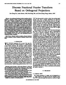
Initially results of applying this approach to synthetic FM signals in noise are presented. Fig 1 illustrates the process of forming the ppCFT for a synthetic LFM signal in Gaussian white noise. Horizontal lines through this plot represent individual CFTs for different chirp-rates. The central line, a chirp-rate of zero, corresponds to the classical FT. It can be seen that along this line the signal energy is not concentrated, but smeared across many frequency bins. Whereas along the line corresponding to the signal’s true chirp rate (60 Hz/s) the energy in the representation is concentrated and a strong peak; the ppCFT extracts this single line as the output spectrum. Fig 2 shows spectrograms based on the FT and ppCFT for a synthetic signal, consisting of a quadratically frequency modulated sinusoid embedded in Gaussian white noise. The largest value occurring in the FT spectrogram occurs when the signal is approximately tonal at t = 0.5 s; with the level of the spectrogram falling progressively as the chirp rate departs from zero. The ppCFT is more robust to these phenomena; the level of the representation is almost constant over the

defines the rate of frequency modulation of the basis functions. Equivalently, one can define an angle ϕ = πα/2 which can be regarded as angle of rotation of the time-frequency plane. Z 2 2 X α (u) =A x(t)eiπ(t cot ϕ−2ut csc ϕ+u cot ϕ) dt p A = 1 − i cot ϕ

(2)

This work concentrates on the problem of signal detection based on the (squared) magnitude of the FrFT and therefore one can use an intuitively appealing and efficient transform, referred to the as the Chirp Fourier transform (CFT) [9] (3). The CFT consists of pre-multiplying the input signal by a synthetic LFM signal of the form exp(−2πiat2 ), prior to taking a FT. To illustrate, consider a LFM signal with known chirp-rate, if it is multiplied by a chirp whose rate is the negative of that in the signal, then the resultant signal is sinusoidal and suited to detection using the FT. Z 2 Xc,a (f ) = x(t)e−2πi(f t+at ) dt (3) It is important to note that the multiplying chirp, exp(−2πiat2 ), should have a mean frequency of zero, which is the case assuming that the data is evaluated on a centred interval, [−T /2, T /2]. The zero mean frequency condition ensures that in forming the product, the frequency the signal being analysed is not altered. It can be shown [8], [10] that the CFT and FrFT can be related in the following manner 2

Xα (u) =Aeiπu cot(ϕ) Xc,a (u csc(ϕ)) |Xc,a (u csc(ϕ))|2 |Xα (u)|2 = | sin(ϕ)|

(4) (5)

Fig. 1. Image of the CFTs using the full range of chirp rates, for the signal exp (2πi(30t2 + 130t)) in Gaussian white noise.

signal’s duration. Further the width of the line representing the signal is considerably narrower in this representation, i.e. the signal’s the energy is concentrated in a few frequency bins. This example demonstrates that the ppCFT also alters the appearance of the background noise compared to the FT, in particular the noise becomes textured in a manner that reflects the direction of the chirp in the signal.

of a detector is achieved by computing receiver operating characteristics (ROC) curves. The computation of a ROC curve is not well suited to performance comparisons employing measured data sets. Consequently in this study, wherein it is desired to draw conclusions regarding the two methods using measured data sets of cetacean vocalisations, an alternative metric is employed. The approach taken is to first identify a detection threshold which corresponds to a predetermined false alarm rate. The ratio (computed as a difference in levels expressed in dB) between the peak level of the signal and this threshold is then evaluated. This ratio defines the attenuation the signal could have undergone before detection would not have occurred. Using this approach a correction factor can be defined when comparing two methods. This correction factor is the ratio between the two thresholds, expressed in dB, for the two methods at the selected false alarm rate. By subtracting this correction factor from the results of the appropriate method a fair comparison can be undertaken. In order to determine the detection thresholds, and hence the correction factors, the statistics of the methods for noise only data need to be evaluated. This can be achieved for the case of Gaussian white noise; which, then imposes the need for a pre-whitening step in the analysis of the measured data sets. A. Threshold for the FT The statistics of the FT of Gaussian white noise are known to conform to an exponential distribution [13], [14], [15], [3], specifically, the threshold, Λf a , expressed in dB, that realises a false alarm rate, Pf a , can be shown to be Λf a = 10 log10 (−σ 2 ln(Pf a ))

(6)

B. Threshold for the ppCFT

Fig. 2. A comparison between the FT spectrogram and the ppCFT for the signal exp (2πi(−2048t3 + 3072t2 )) in Gaussian white noise (fs = 4096 Hz). The spectrograms are computed using a Hanning window of length 512 .points and overlapped by 87.5%

V. M ETHOD OF E VALUATION The results from the preceding section suggest that the ppCFT may be well suited to the detection of FM signals. Specifically the concentration of energy in such signal to a few frequency bins, even when the chirp rate is high, means that such bins should be prominent relative to the noise floor. In order to determine whether such an apparent performance advantage can be realised in a practical system a suitable measure of performance needs to be selected and evaluated. Probably the most complete evaluation of the performance

Unlike the FT, the statistics of the ppCFT for Gaussian white noise inputs have not been previously been detailed. This section evaluates those statistics through Mont´e-Carlo simulations. The individual CFTs for a fixed chirp rate have exactly the same distribution as the FT, i.e. an exponential distribution. However, the statistics of the ppCFT of Gaussian white noise differ significantly from the individual CFTs. This is a consequence of the peak-picking process which selects the value of a generating the largest single value from a set of N + 1 CFTs computed with different a’s. Consequently, by definition, the selected CFT necessarily includes, at least, one unusually large value. Fig 3 has been obtained through Mont´e-Carlo simulation. The plot illustrates the probability of false alarm against spectral level for the ppCFT for different window lengths. Therefore for the ppCFT, assuming unit variance white noise, the thresholds for false alarm rates of 10−4 and 10−5 are now dependent on block size, but for 1024 points the thresholds are 11.44 dB and 12.11 dB respectively. The difference between this level and the level associated with the FT is the correction factor that needs to be applied to equalise the false alarm rates

trum using the method described in [16], and filtering using an inverse filter. Then a period containing a suitable narrowband FM component is identified. That period is analysed using the spectrogram and short-time ppCFT methods, with the optimised window size. For the ppCFT the correction values in Table I are applied. TABLE II P ERFORMANCE SUMMARY

Signal

Fig. 3.

Probability of False Alarm for the ppCFT

. of the two methods and so render the comparison fair. For 1024 points the correction factors for false alarm rates of 10−4 and 10−5 are 1.8 dB and 1.5 dB respectively. Table I summarises these correction factors for a range of block sizes. TABLE I C ORRECTION FACTORS FOR THE PP CFT FOR A VARIETY OF BLOCK - SIZES

Block-size (N ) 256 512 1024 2048 4096 8192

Correction Factor (dB) Pf a = 10−4 Pf a = 10−5 1.1 1.0 1.4 1.2 1.8 1.5 2.0 1.7 2.2 1.9 2.3 2.0

VI. R ESULTS The ppCFT and FT are compared mainly on the basis of a number of recordings from various cetacean species which utilise narrow-band FM vocalisations. It should be noted that there are a large number of cetacean species that produce narrow-band vocalisations and that some of the species have diverse vocal repertoires. Consequently the data set analysed here only aims to capture a few typical examples. The comparison between the ppCFT and FT spectrograms allows for the fact that the performance of each method depends upon the chosen window size. A fair comparison for each data sample should allow the methods to optimise this window length independently. To this end both methods analyse the data using a range of window sizes with the spectrograms being normalised so that the thresholds are independent of the different of window size. The spectrogram that yields the largest value is then selected as the best for that method, for that data. The analysis of the cetacean recordings starts by prewhitening the data, i.e. estimating the background noise spec-

Synthetic Tonal LFM Odontocetes Atl. Whitesided Dolphin (Lagenorhynchus acutus) Bottlenose Dolphin (Tursiops truncatus) a b Dusky Dolphin (Lageno. obscurus) a b Pantropical Spotted Dolphin (Stenella attenuata) a b c Killer Whale (Orcinus orca) Mysticetes Fin Whale (Balaenoptera physalus)

Chirp Rate (kHz/s)

Best FT Size

Best ppCFT Size

ppCFT Gain (dB)

0 4

8192 1024

8192 8192

-2.0 6.3

-36.6

2048

4096

2.2

54.3 -10.4

512 1024

4096 4096

2.1 3.1

-10.7 14.3

1024 1024

4096 2048

2.6 1.0

15.3 8.4 35.9

2048 1024 2048

2048 4096 4096

-1.0 -0.5 1.2

9.74

2048

4096

0.8

-0.003

512

512

-1.2

Table II details the performance gain (in dB) of the ppCFT over the FT for a probability of false alarm of 10−5 . Negative values relate to a degradation in detectability, i.e. a performance loss when using the ppCFT. The synthetic data provides results that one might expect: the FT offers the best performance for a tonal signal, whereas for a LFM signal it is the ppCFT which achieves best performance. For the recorded data, the benefit of using the ppCFT is dependent on how well the vocalisations conforms to the LFM model. In general the detectibilty for the cetacean data is significantly less than that for the synthetic synthetic data, reflecting the fact that these vocalisations are not exactly modelled as LFM signals. For the signals considered the improvement in detectability ranges from -1.2 to 3.1 dB. The best improvement is generally associated with the whistles with the fastest chirp-rates, as one might anticipate. The optimal window length of the ppCFT is never smaller than the FT window length and in most cases is significantly longer. Some of the variability can be explained by considering the character of the signals. In particular the whistles of the pantropical spotted dolphin contain short sections where the chirp rate is close to zero and the performance advantage of the ppCFT over the FT is compromised. The dusky dolphin data is recorded at a relatively low SNR and in reverberant environment, this, to a lesser extent, also compromises the

ppCFT. The fin whale call, which has a relatively low chirp rate, is poorly suited to analysis with the ppCFT. VII. C ONCLUSION The results show that for cetacean tonal vocalisations, the theoretical performance of the FrFT is difficult to realise primarily because a real signal will not precisely obey a linear frequency law. However for these signals the FrFT can offer modest gain of up to about 3 dB, the method also produces an estimate of signal chirp rate within the spectrogram data block. Future work will aim to exploit this feature to produce a frequency line tracking scheme based on measurements of instantaneous frequency and chirp rate. It is believed that this approach will mitigate some of the track seduction effects commonly seen in tracking algorithms. A successful tracking solution will allow the extraction of FM tonal features from the spectrogram, these features can be used to characterise or classify the sound source and determine whether the source is man-made or biological. VIII. ACKNOWLEDGMENT The Authors would like to thank Jennie Johnson of Dstl Naval Systems and Paul Thomas and Steve Benn of the University Defence Research Centre on signal processing for their support and advice. c

British Crown copyright - DSTL 2010 - published with the permission of the Crontroller of Her Majesty’s Stationery Office R EFERENCES [1] J. N. Oswald, S. Rankin, J. Barlow, and M. O. Lammers, “A tool for real-time acoustic species identification of delphinid whistles,” The Journal of the Acoustical Society of America, vol. 122, no. 1, pp. 587– 595, 2007. [Online]. Available: http://link.aip.org/link/?JAS/122/587/1 [2] S. Datta and C. Sturtivant, “Dolphin whistle classification for determining group identities,” Signal Process., vol. 82, no. 2, pp. 251–258, 2002. [3] H. van Trees, Detection estimation, and modulation theory, Pat 1. Wiley & Son, 2002. [4] R. Nielson, Sonar Signal Processing. Artech House, 1991. [5] L. Cohen, “Time-frequency distributions-a review,” Proceedings of the IEEE, vol. 77, no. 7, pp. 941 –981, jul 1989.

[6] J. Hammond and P. White, “The analysis of non-stationary signals using time-frequency methods,” Journal of Sound and Vibration, vol. 190, no. 3, pp. 419–447, FEB 29 1996. [7] C. Capus and K. Brown, “Short-time fractional fourier methods for the time-frequency representation of chirp signals,” J. Acoust. Soc. Am., vol. 113, pp. 3253 –3263, 2003. [8] A. Zayed, “On the relationship between the fourier and fractional fourier transforms,” Signal Processing Letters, IEEE, vol. 3, no. 12, pp. 310 – 311, dec 1996. [9] J. Locke, “Detection performance of the chirp-fft (fractional fourier transform) for marine mammal vocalisations,” Master’s thesis, ISVR, University of Southampton, 2009. [10] L. Almeida, “The fractional fourier transform and time-frequency representations,” IEEE Trans. Signal Process, vol. 42, pp. 3084–3091, 1994. [11] C. Capus, “Time-frequency methods based on the fractional fourier transform,” Ph.D. dissertation, Dept of Computing and Electrical Engineering, Heriot-Watt University., 2002. [12] I. Stevenson, P. Nicholson, L. Linnett, and S. Morrison, “A method for the analysis of chirp signals insonifying layered media for sub-bottom profiling,” MTS/IEEE Oceans, pp. 2608–2615, 2001. [13] A. Whalen, Detection of signals in noise. London, UK: Academic, 1971. [14] G. Brethorst, Bayesian spectrum analysis and parameter estimation. Springer-Verlag, 1988. [15] A. Papoulis and S. Pillai, Probability, random variables and stochastic processes (4th Ed). McGraw-Hill, 2002. [16] T.-T. Leung and P. White, Mathematics in Signal Processing IV. Clarendon Press, 1998, ch. Robust estimation of oceanic background noise spectrum, pp. 369–382.