The two leading approaches for detecting multiple instances of an object class in an image are sliding ... the most notable is the cascaded evaluation [1,6] where each stage employs a ... Let P(Ck) be the prior on class Ck which can be estimated ... ing the Eye in a frontal human face is a natural part, yet people wear glasses.
The Semi-explicit Shape Model for Multi-object Detection and Classification� Simon Polak and Amnon Shashua School of Computer Science and Engineering The Hebrew University of Jerusalem
Abstract. We propose a model for classification and detection of object classes where the number of classes may be large and where multiple instances of object classes may be present in an image. The algorithm combines a bottom-up, low-level, procedure of a bag-of-words naive Bayes phase for winnowing out unlikely object classes with a high-level procedure for detection and classification. The high-level process is a hybrid of a voting method where votes are filtered using beliefs computed by a class-specific graphical model. In that sense, shape is both explicit (determining the voting pattern) and implicit (each object part votes independently) — hence the term ”semi-explicit shape model”.
1
Introduction
One of the great challenges facing visual recognition is scalability in the face of large numbers of object classes and detected instances of objects in a single image. The task requires both classification, i.e., determine if there is a class instance in the image, and detection where one is required to localize all the class instances in the image. The scenario of interest is where a class instance occupies a relatively small part of the image surrounded by clutter and other instances (of the same class and other classes), and all of that in the face of a large number of classes, say hundreds or thousands. The two leading approaches for detecting multiple instances of an object class in an image are sliding windows (cf. [1,2,3]), and voting methods (cf. [4,5]), which are based on modeling the probabilities for relative locations of object parts to the object center or more generally to the Hough transform. The sliding-window approach applies the state-of-the-art binary (”one versus many”) classification in a piece-meal fashion systematically over all positions, scale and aspect ratio. The computational complexity of this scheme is unwieldy although various techniques have been proposed to deal with this issue where the most notable is the cascaded evaluation [1,6] where each stage employs a more powerful (and expensive) classifier. Controlling the false positive rate, given the very large number of classification attempts per image, places considerable challenges on the required accuracy of the classifier and is typically dealt by means of post-processing such as non-maximal suppression. �
This work was partially funded by ISF grant 519/09.
K. Daniilidis, P. Maragos, N. Paragios (Eds.): ECCV 2010, Part II, LNCS 6312, pp. 336–349, 2010. c Springer-Verlag Berlin Heidelberg 2010 �
The Semi-explicit Shape Model for Multi-object Detection and Classification
337
In contrast to this, the voting approach parametrizes the object hypothesis (typically, the location of the object center) and lets each local part vote for a point in hypothesize space. These part-based methods combine large numbers of local features in a single model by establishing statistical dependencies between parts and the object hypothesis, i.e., by modeling the probabilities for relative locations of parts to the object center [4]. In some cases, the spatial relationship among the parts are not modeled thereby modeling the object as a ”bag of parts” as in the Implicit Shape Model (ISM) of [4] and in other cases shape is represented by the mutual position of its parts through a joint probability distribution [7,8,9,10]. The ISM approach is efficient and is designed to handle multiple instances of an object class, however, the lack of shape modeling contaminates the voting map with multiple spurious local maxima [5]. The probabilistic models on the other hand require a daunting learning phase of fitting parameters to complex probabilistic models although various techniques have been proposed to deal with the complexity issue such as identifying ”landmark” parts [9,10] or Tree-based part connectivity graphs [8]. Moreover, the probabilistic models lack the natural ability to handle multiple instances in parallel (like ISM does), although in some cases authors [8] propose detecting multiple instances in a sequential manner starting from the ”strongest” detected model after which nearby parts are excluded to find the best remaining instance and so on. Finally, both ISM and the explicit shape models would be challenged with increasing number of object classes as there is no built-in filters for winnowing out the less likely object classes given the image features before the more expensive object-class by object-class procedures are applied. Our proposed model combines a bottom-up ”bag of parts” procedure using a naive Bayes assumption with a top-down probabilistic model (per object class). The probabilistic model, on one hand, represents the shape by interconnection of its parts and uses approximate inference over a loopy graphical model to make inference. However, the inference results are not used explicitly to match a model to an image but implicitly to filter out the spurious votes in the ISM procedure. The voting of parts to object centers are constrained by the marginal probabilities computed from the graphical model representing the object shape. Therefore, spurious parts not supported by neighboring parts according to the shape graph would not vote. Furthermore, the locations of maximal votes are associated with a classification score based on the graphical model rather than by the amount of votes. Because shape is used both explicitly and implicitly in our model we refer to the scheme as ”semi explicit shape model”.
2
The Semi-explicit Shape Model
Let C1 , ..., Cn stand for the n object categories/classes we wish to detect and locate in novel images. Let P (Ck ) be the prior on class Ck which can be estimated from the training set (number of images we have from Ck divided by the size of the training set). We assume that for each class we have a set of training images where the object is marked by a surrounding bounding box. We describe
338
S. Polak and A. Shashua
below the training phase which consists of creating a code-book of features, defining object ”parts” and their probabilistic relation to code words, and the construction of Part connectivity graph per object class. Following the training phase we describe in Section 2.2 the details of our classification and detection algorithm. 2.1
The Training Phase
We start the training phase by constructing a ”code book” W by clustering all the descriptors gathered around all interest-points from all the training images. From the training images of the k’th object class we perform the following preparations: (i) delineate the Parts of the object each consisting of a 2D Gaussian model and the collection of interest points and their descriptors associated with the Part, (ii) a Part neighborhood graph which would serve during the visual recognition phase as a graphical model for enforcing global spatial consistency among the various Parts of the object, and (iii) construct the probabilistic representation of object Parts by the conditional likelihood P (R | w) for all w ∈ W. We present each step in more details below. The Code Book: all training images are passed through a difference of Gaussians interest point locator and a SIFT [11] shape descriptor vector is generated per interest point and per scale. The area under each bounding box is represented at different scales and recorded with each descriptor. We use an agglomerative clustering algorithm (such as the Average-Link in [12]) to group together descriptors of similar shape and of the same scale. An agglomerative clustering bounds the quantization error (which in turn is bounded by the threshold distance parameter between descriptors) and allows to represent isolated descriptors (such as those generated by object-specific image fragments) as clusters. A K-means clustering approach, although superior computational-wise, would force isolated descriptors to get associated with some larger cluster of common descriptors, thereby increasing the quantization error. The i’th cluster is denoted by wi and consists of the descriptor vectors di1 , ..., dimi and the average descriptor di where mi is the cluster size. Each code word is associated with some scale (as the clustering is performed for each scale separately). The code-book W is the set of ”code words” wi (s), i = 1, ..., M and s is the scale label. Object Parts Delineation: we define an object ”part” by a concentration of interest points, collected over all the training images of the class. We do not require the interest points to share similar descriptors in order to allow for appearance variability within the scope of the Part. For example, the area surrounding the Eye in a frontal human face is a natural part, yet people wear glasses which renders the appearance of that area in the image undergo considerable variation. On the other hand, our working assumption is that concentrations of interest-points undergo only moderate variability. Thus, radically different viewing positions of an object, for example, are not currently included in our model of an ”object class”. The point concentrations are detected and modeled as
The Semi-explicit Shape Model for Multi-object Detection and Classification
339
Fig. 1. Examples of model Parts for some classes of Caltech101 database. Each ellipse depicts a 2D Gaussian associated with a separate Part.
follows. Given all the training images of class Ck , the bounding boxes around the object are scale-aligned and interest point locations are measured relative to the bounding-box center (object center). The collected interest-points over all the training images of Ck are fed into a Gaussian-Mixture-Model (GMM) using the Expectation-Maximization algorithm [13]. The number of Parts (Gaussian models) is determined by a minimum-description-length principle described in [14]. The result is a list of Parts Rjk represented by N (μkj , Σjk ) a 2D Gaussian model, for j = 1, ..., nk where nk is the number of Parts of object class Ck . Note that we have tacitly assumed that scale does not influence the Part structure of the object (number and shape distribution). The assumption holds well in practice under a large range of scales and simplifies the algorithm. Fig. 1 illustrates the Parts found in some of the Caltech101 images. k which consists of the set of We define for each class a ”context” Part RB descriptors from interest points located in the vicinity of the object bounding box and collected over all the training images of Ck . The Context Part will be used in the next section as additional evidence for the likelihood of Ck given a novel image. In addition, let Fjk be the set of descriptors of the interest points which were assigned by the GMM algorithm to Part Rjk . Since GMM provides a probabilistic assignment of interest points to Parts, each interest point can belong to more than one Part. We leave only the strong (above threshold) assignments, i.e., each interest point is associated with the highest probability Parts. Finally, let � F k = j Fjk stand for the set of all descriptors of interest points of class Ck , � and F = k F k the set of all descriptors collected from the training set. Probabilistic Representation of Parts P (Rjk | wi ): we wish to represent the Part Rjk by its conditional probability given a word wi . Such a representation is useful for determining the likelihood of having Rjk in an image given interest points and their SIFT descriptors which in turn can be used to obtain a preliminary classification score based on a naive Bayes model. To compute P (Rjk | wi ), let |Fjk ∩ wi | denote the number of descriptors that are in both the part Rjk and the code word wi . The ratio |Fjk ∩ wi |/|wi | is not a good representation of P (Rjk | wi ) because it makes a tacit assumption that the
340
S. Polak and A. Shashua
prior P (Ck ) is equal to |Fk |/|F | the relative number of descriptors from Ck — an assumption that is obviously wrong. � We expand P (Rjk | wi ) while noting that P (Rjk | Ck ) = 0 when k � �= k: P (Rjk | wi ) = P (Rjk | Ck , wi )P (Ck | wi ) = P (Rjk | Ck , wi ) |Fjk ∩ wi | = k |F ∩ wi |
P (wi | Ck )P (Ck ) P (wi )
|F k ∩wi | P (Ck ) |F k |
|wi |/|F |
Note that if we substitute |Fk |/|F | for P (Ck ) we obtain the ratio |Fjk ∩ wi |/|wi |. Following the cancelation of the term |F k ∩ wi | we obtain: P (Rjk | wi ) =
|Fjk ∩ wi | · |F | · P (Ck ) |Fk | · |wi |
(1)
k Note that the definition above applies to P (RB | wi ) as well where Fjk is replaced k by FB the set of descriptors of the Context Part.
Constructing the Part Connectivity Graph: an explicit shape model of class Ck is represented by a connected (undirected) graph G(V k , E k ) whose set of nodes V k correspond to the Parts Rjk , j = 1, ..., nk and whose set of edges E k defines the ”Part neighborhood” to guarantee a global consistency structure among the Parts. The neighborhood relations are determined by a Delaunay triangulation [15] over the Gaussian centers μkj which form the Part centers. 2.2
Detection and Recognition of Object(s) Instances in a Novel Image
The training phase described above has generated (i) a code book W where each word w(s) ∈ W represents a set of image descriptors of similar appearance and scale s, (ii) the j’th object Part Rjk of class Ck represented by a 2D Normal distribution in object-centered coordinates, (iii) a ”bag of words” association between object Parts Rjk and code words wi represented by the scalar P (Rjk | wi ) (eqn. 1), and (iv) a Part connectivity graph. Given a novel image I we wish to detect and recognize instances of the object classes C1 , ..., Ck allowing for multiplicity of objects and multiplicity of instances of each object at different scales. The detection and classification process has two phases: – A low-level, bottom-up, ”bag of words” based classification of object classes. Classification is based on the association P (Rjk | wi ) over all code-words and Parts of each object class. Classification also forms a ranking of the possible object classes thereby allowing the system to focus its high-level resources on the most likely object classes that may be present in the image first.
The Semi-explicit Shape Model for Multi-object Detection and Classification
341
– A high-level classification and detection process: for each of the likely classes Ck , the Part connectivity graph is matched to the image using a TreeReweighted (TRW) approximate inference over a loopy graphical model. Each Part obtains ”beliefs” on its possible locations in the image (allowing for multiple instances). The Part locations with high Belief vote for the respective object-class center. The result is a ”heat map” (like with the ISM method) of possible centers of instances from Ck . Each object-center candidate in the heat-map is associated with a score given by the graphical model inference which serves as a high-level classification score. This high-level process is performed sequentially over each object-class limited to those classes with high likelihood (as determined by the low-level phase). We describe the two phases in detail below. Likelihood of Classes as a Low-Level Process: the low-level classification process is triggered from detected interest points and their associated SIFT descriptors from the novel image. A nearest-neighbor search is performed to match the descriptor of each interest point to a code-word. Because of the relatively high dimension of the SIFT descriptor we use the locally-sensitive-hashing (LSH) method based on random projections [16]. Let wI be the subset of code words present in the input image, then the conditional likelihood P (Rjk | I) of the Part Rjk existing in novel image I is: � P (Rjk | I) = P (Rjk | wi )P (wi | I), wi ∈wI
and the conditional log-likelihood log P (Ck | I) of the class Ck given the novel image is determined by a Naive Bayes approach: log P (Ck | I) =
nk �
k log P (Rjk | I) + log P (RB | I),
(2)
j=1 k where RB is the Context part (defined above). The probabilistic representations above are ”bag of words” type of inference where the likelihoods of Parts and object classes depend only on the existence of features (code words) and not through their spatial interconnection. The inference of log P (Ck | I) follows from a Naive-Bayes assumption on a co-occurrence relation between objects and parts. This ”weak” form of inference is efficient and allows us to perform a preliminary classification which also serves as a ranking of the possible classes by means of log P (Ck | I). A similar approach of using nearest-neighbors with a naive-Bayes approach (but without a code book and other details of Parts and their probabilistic relation to code words) was introduced by [17].
High-level Classification and Detection: this phase is performed on each object class Ck whose classification score log P (Ck | I) was above threshold, i.e., the high-level process focuses its resources on the most likely object classes first. We
342
S. Polak and A. Shashua
construct an inference problem defined by a joint probability P (xk1 , ..., xknk ) using the connectivity graph G(V k , E k ) for defining direct interactions among the variables. The variable xkj is defined over a finite set of values representing the possible locations of the Part Rjk in the image. The marginal probability distribution P (xkj ) represents the probability (”belief”) P (xkj = r) for Rjk to be found in location r in the image. Each possible location r votes to Ck ’s object center if P (xkj = r) is above threshold. The result of the voting process is a ”heat-map” for instances of Ck in the image. The value of P (xk1 = r1 , ..., xknk = rnk ) provides a classification score of an instance of Ck at a specific location in the image where, unlike the low-level phase where the score was based on a ”bag-of-words” setting, the score is based on satisfying the connectivity constraints among object parts. We therefore have both detection (via the heat-map) and classification achieved simultaneously. We present the scheme in more details as follows. Let I = I1 , ..., IM be the set of interest points and their associated descriptors located in the novel image and let w1 , ..., wM the corresponding codewords (found using LHS nearest-neighbor approximation). Let Ijk ∈ I be the subset of interest points for which their corresponding code-words wi satisfy P (Rjk | wi ) > � for some threshold �. In other words, the set Ijk are the interest points in the novel image that are likely to belong to the Part Rjk . We perform agglomerative clustering on Ijk where the similarity measure is the Mahalanobis distance with zero mean and covariance matrix of Rjk (recall that each Part is associated with a Normal distribution) for each pair arising from the same scale and infinity otherwise. Since each code word has an associated scale, interest points arising from different scales will not be clustered together. Let nkj be the number of clusters found and γ1 , ..., γnkj are the clusters of the respective code words associated with Ijk and l1 , ..., lnkj are the geometric centers of the clusters.
Let xkj ∈ {1, ..., nkj } be a random variable associated with the possible locations of the Part Rjk (where each location is a cluster of interest points of scale s for which P (Rjk | wi (s)) > � ). The joint probability distribution over the variables xkj , j = 1, ..., nk has the form: nk � 1 � φj (xkj ) ψi,j (xki , xkj ), (3) P (xk1 , ..., xknk ) = Z j=1 k (i,j)∈E
where φj (xkj ) represents the ”local evidence”, i.e., φj (xkj = r) is the probability that Rjk is located at location r from local evidence alone: φj (xkj = r) = 1 −
� � wi ∈γr
� 1 − P (Rjk | wi ) ,
and ψi,j (xki , xkj ) are the pairwise ”potential” functions on pairs of Parts that are incident in the connectivity graph. The value of ψi,j (xki = r, xkj = q) represents the likelihood that the two Parts are located in positions r, q (and scale s) respectively:
The Semi-explicit Shape Model for Multi-object Detection and Classification
343
Fig. 2. Each image shows a Part Rjk (Red Ellipse) with the set of candidate locations xkj . Locations with high belief are those who vote and are drawn with an arrow pointing to the object center. The beliefs generated by the graphical model form a strong constraint on the voting pattern of Part candidates so that only those locations who have global shape support end up voting. The images contain multiple instances thus the belief pattern of P (xkj ) is multi-modal. Candidate locations from both object instances end up voting.
ψi,j (xki = r, xkj = q) = N (lr − lq ; μij , Σij ), where μij , Σij is the scaled difference Normal distribution where μij = (μki −μkj )s and Σij = (Σik + Σjk )s2 . We set ψ() = 0 in case positions r, q are associated with different scales. The marginal probabilities P (xkj ) hold the likely Part locations, i.e., if P (xkj = r) is above threshold then we have a certain ”belief” that lr (the geometric center of γr the r’th cluster) is where the Part Rjk is centered. Because we may have multiple instances of Ck in the image, P (xkj = r) may have a multi-modal profile where more than a single Part location is supported by the connectivity graph. Computing the marginal probabilities is computationally infeasible and instead we resort to ”approximate inference”. Since the connected graph has loops, the sum-product Belief-Propagation (BP) algorithm is not guaranteed to converge. Moreover, regardless of convergence, the BP algorithm tends to settle on single-modal beliefs, i.e., P (xkj ) will come out single-modal even when multiple instances of Ck exist in the image. We used the Tree-reweighted (TRW) convexfree-energy variational approximation which is both guaranteed to converge and is not limited to single-modal solutions. Specifically, we used the sum-TRBP [18] implementation (even though convergence is not guaranteed). Convergence guaranteed TRW algorithms (and general convex-free-energy) can be found in [19]. The marginal probabilities P (xkj ) play two roles in the high-level detection and classification process. First is to ”clean up” the voting of Part candidates to object centers, and second to obtain a high-level (shape-based) classification score for each detected instance of Ck in the image. Those are detailed below. Voting: once the (approximate) marginal probabilities P (xkj ) are estimated we perform a voting procedure: For each Part Rjk , the candidate Part centers lr will vote to the respective object center if P (xkj = r) is above threshold. Fig. 2 illustrate the constrained voting procedure: in each image a Part is shown marked by an Ellipse and all candidate locations for the Part are marked by circles. Only
344
S. Polak and A. Shashua
Fig. 3. From heat-map to classification score: the middle column shows the heat map generated by ISM (i.e., without our high-level filtering using beliefs generated from sum-TRBP). The third column shows the heat-map generated by our algorithm. It is evident that most of the voting contamination has been removed. The centers of maximal votes found by Mean-Shift are marked on the heat-maps. The righthand column shows the classification score (generated by the joint probability distribution) associated with each of the heat map centers. The top and bottom rows show the cases where the class is the correct one and one can see that the true heat map center has the (significantly) highest classification score (No. 5 in top, and 5,6 in bottom). The middle row shows a case where the class is not found in the image. In that case all classification scores are close to zero (the scale is 10−3 ).
those locations which received high belief make a vote and are displayed with an arrow towards the object center. It is evident than only a small fraction of the possible locations eventually make a vote and that the procedure is able to concentrate on both instances simultaneously due to the usage of the sum-TRBP algorithm. In other words, the voting process is a ”filtered” version of the ISM method. Rather than having all Part candidates vote for their respective object center, only those candidates with high Belief perform the voting. This ”high-level filter” has a dramatic effect on reducing the ”clutter” formed by spurious votes on the resulting object-centers ”heat map” (see Fig. 3). High-level Classification: the voting process creates a heat-map where locations having many votes are likely to form centers of instances of Ck , thus the ”strength” of a candidate instance can be directly tied to the number of votes the center has received — this is the underlying premise of ISM. However, we can do better and obtain a classification measure by evaluating P (xk1 , ..., xknk ) for every instance candidate (a center receiving sufficient votes), as follows. Consider a candidate center c and the set of locations Lc which have voted to it. Each location is associated with a Part Rjk and with a value of its corresponding position label xkj . Let Lc (j, k) ⊂ Lc be the locations corresponding to Rjk and let r1 , ..., rb be the values of xkj corresponding to the locations Lc (j, k). Normally b = 1, i.e., there is only one location for Rjk and the value of xkj is set accordingly
The Semi-explicit Shape Model for Multi-object Detection and Classification
345
(to r1 ). In case b > 1, then xkj = argmaxq P (xkj = rq ). In case Lc (j, k) = ∅, i.e., Part Rjk did not vote to center c, then xkj is set to the label with maximal belief. Once xk1 , ..., xknk are set to their value, we evaluate P (xk1 , ..., xknk ) according to eqn. 3. The value of the joint probability measure both local fit of Parts and global consistency among parts and therefore serves as our classification score of the candidate instance of Ck at center c. The difference between the Naivebayes score P (Ck | I) (eqn. 2) and the high-level classification score is dramatic at time boosting accuracy of recognition by significant amounts. Fig. 3 shows examples of heat-maps with the maximal centers (estimated using mean-shift procedure) together with the classification scores associated with those centers. It is evident that true center candidates have a much higher classification score than spurious centers (despite them having a similarly large number of votes). In images where the object class is not present, all candidate centers have a low classification score.
3
Experiments
We have tested our model on two standard datasets, Clatech101 [20] and Pascal VOC 2006 [21]. The Caltech101 dataset contains images containing a single dominant object from 101 classes including cars, faces, airplanes, motorbikes among other classes. The instances from those classes appear approximately at similar scale and pose in all images. Each object class is found in between 100 to 800 images. The Pascal dataset is more challenging as it contains 5000 images, split evenly to training and testing subsets, of ten object classes with varying scale and viewpoint where each image may contain multiple instances of object classes. As a result objects are less dominant in the image compared to Caltech101 thereby making the task of detection and classification challenging. Fig. 4 shows the Parts detected in test images by taking the locations of highest belief for each part of the object class in question. One can see the detected Parts agree with their true locations on the test images. With the Calctech101 dataset we performed the object versus other objects categorization experiment, where the goal is to classify an image to one of the 101 object classes. We have removed the F aces easy class, since the objects is this class are identical to the objects in the class F aces, so the number of classes in our experiments was 100. In this test we selected a training set of 15 images per class and a test set of 15 images per class. We collected around 750, 000 features for each object scale (we have used 5 scales) and clustered them into a code book of sizes ranging from 60, 000 to 80, 000 and the number of Parts per object varied between 8 to 15. During the testing phase, each image produced between 100 − 1000 interest points and each part had between 10 − 30 possible locations. Mean running time for a test image was under 5 seconds on a standard 3GHZ CPU. We ran both classifiers: our low-level naive Bayes classifier P (Ck | I) and the high-level detection and classification( in this case the categorization is performed by selecting the class with highest detection score). Table 1 shows comparison of our results to other methods on the Caltech101 dataset.
346
S. Polak and A. Shashua
Fig. 4. Examples of correct detections of classes ’face’, ’car’, ’motorbikes’ and ’airplanes’ from Caltech101 dataset. Each circle in the images represent most probable location of a different Part of the object’s shape model. The Red dots inside the circles are the interest points belonging to this Part. Table 1. Categorization performance comparison our approach and other methods on the Caltech101 dataset Naive Bayes High-Level [17] [22] [23] [24] [25] 51.70% 68.80% 65.00% 59.30% 59.10% 52.00% 56.40%
With the Pascal VOC 2006 dataset, we used the provided training set (of 2500 images) to create a model for each of the four view points of each object and tested our algorithm in both categorization and detection tasks. From the training images of the Pascal database we extracted more then 2,500,000 SIFT features, which resulted in around 100,000 code words for each scale. During the model creation we have used the view information available in the dataset to construct separate models for each of the existing four views (left, right, rear and frontal) in a similar manner to that used for Caltech101. For the classification test, the classification score is computed (by taking the center with the highest classification score from the heat map) per object class. Since an image can contain a number of object classes, an ROC curve is constructed and the area under the curve is taken for the performance measure. Table 2 shows the classification performance of our algorithm for all the ten classes, compared to the low-level naive Bayes phase of our algorithm. In most classes the shape model boosts the performance but in some case, such as with the class of Pedestrians, the performance actually decreases. The reason for that is that Pedestrians instances are sometimes at a very small scale and the system does not detect a sufficient number of interest points to enable the graphical model to perform as expected. On the other hand, those images often contain multiple Pedestrians thus the ”bag of code words” underlying the naive Bayes procedure collects evidence from the multiple instances. For the detection task, performance is measured by the overlap between bounding boxes. Fig. 5 shows some detection results on a sample of test images
The Semi-explicit Shape Model for Multi-object Detection and Classification
347
Table 2. Performance comparison between the high-level classification and the naive Bayes low-level classification on the Pascal VOC 2006 dataset bicycle bus car cat cow dog horse motorbike person sheep High-Level 90% 93% 90.9% 85.4% 88.5% 77.3% 72.4% 86.4% 60% 87.3% Naive Bayes 87.3% 90.7% 89% 82.5% 85.9% 75.7% 68.4% 78.7% 67.7% 82.7%
Fig. 5. Examples of detections from the Pascal VOC 2006 dataset (see discussion in text) Table 3. Performance comparison between the proposed algorithm and published results by other methods (sliding window and voting) on the Pascal VOC 2006 dataset
Our Cambridge ENSMP INRIA Douze INRIA Laptev TUD TKK FeiFei09] Felzenszwalb’09
bicycle 0.36 0.249 0.414 0.44 0.303 0.619
bus 0.184 0.138 0.117 0.169 0.49
car 0.621 0.254 0.398 0.444 0.222 0.310 0.615
cat 0.171 0.151 0.160 0.188
cow 0.39 0.149 0.159 0.212 0.224 0.252 0.407
dog 0.18 0.118 0.113 0.151
horse 0.37 0.091 0.140 0.137 0.392
motorbike 0.55 0.178 0.390 0.318 0.153 0.265 0.576
person 0.33 0.030 0.164 0.114 0.074 0.039 0.363
sheep 0.41 0.131 0.251 0.227 0.404
where we can see the ability of the algorithm to handle occlusions, view and scale variations and multiple instances of an object appearing in the same image. Table 3 summarizes the detection performance of our algorithm in comparison to other methods. As it can be seen from the table our system outperforms many methods on most of the classes except the sliding-window method by [3]. The running time per image in the Pascal dataset is less than 4 seconds compared to much longer running times by other methods.
4
Summary
We described an object detection and classification scheme based on a voting mechanism. Our system starts with a bottom-up Naive-Bayes ”bag of words”
348
S. Polak and A. Shashua
classification for ranking the possible class models present in the image followed by a top-down voting of visual code words (through Parts) to potential object classes. The voting mechanism is filtered by explicit shape models represented by graphical models. The ”beliefs” computed by each of the graphical models leave intact votes from code-words which gain structural support by other code-words in the graph. The system is designed to scale gracefully with the number of classes and achieves comparable, and often superior, detection and classification accuracies than other systems which have a considerably higher run-time.
References 1. Viola, P., Jones, M.: Rapid object detection using a boosted cascade of simple features. In: Proceedings of the IEEE Conference on Computer Vision and Pattern Recognition, pp. 511–518 (2001) 2. Dalal, N., Triggs, B.: Histograms of oriented gradients for human detection. In: Proceedings of the IEEE Conference on Computer Vision and Pattern Recognition, pp. 886–893 (2005) 3. Felzenszwalb, P., McAllester, D., Ramanan, D.: A discriminantly trained, multiscale, deformable part model. In: Proceedings of the IEEE Conference on Computer Vision and Pattern Recognition (2008) 4. Leibe, B., Leonardis, A., Schiele, B.: Combined object detection and segmentation with an implicit shape model. In: ECCV 2004 Workshop on Statistical Learning in Computer Vision (2004) 5. Ommer, B., Malik, J.: Multi-scale object detection by clustering lines. In: Proceedings of the International Conference on Computer Vision (2009) 6. Vedaldi, A., Gulshan, V., Varma, M., Zisserman, A.: Multiple kernels for object detection. In: Proceedings of the International Conference on Computer Vision (2009) 7. Fergus, R., Perona, P., Zisserman, A.: Object class recognition by unsupervised scale-invariant learning. In: Proceedings of the IEEE Conference on Computer Vision and Pattern Recognition (2003) 8. Felzenszwalb, P., Huttenlocher, D.: Pictorial structures for object recognition. International Journal of Computer Vision 61, 55–79 (2005) 9. Fergus, R., Perona, P., Zisserman, A.: A sparse object category model for efficient learning and exhaustive recognition. In: Proceedings of the IEEE Conference on Computer Vision and Pattern Recognition (2005) 10. Crandall, D., Felzenszwalb, P., Huttenlocher, D.: Spatial priors for part-based recognition using statistical models. In: Proceedings of the IEEE Conference on Computer Vision and Pattern Recognition (2005) 11. Lowe, D.G.: Distinctive image features from scale-invariant keypoints. International Journal of Computer Vision 60, 91–110 (2004) 12. Leibe, B., Mikolajczyk, K., Schiele, B.: Efficient clustering and matching for object class recognition. In: British Machine Vision Conference, BMVC 2006 (2006) 13. Dempster, A., Laird, N., Rubin, D.: Maximum likelihood from incomplete data via the em algorithm. Journal of the Royal Stat. Soc., Series B 39, 1–38 (1977) 14. Wallace, C.S., Freeman, P.R.: Estimation and inference by compact coding. Journal of the Royal Statistical Society. Series B (Methodological) 49, 240–265 (1987) 15. Cignoni, P., Montani, C., Scopigno, R.: Dewall: A fast divide and conquer delaunay triangulation algorithm in ed . Computer-Aided Design 5, 333–341 (1998)
The Semi-explicit Shape Model for Multi-object Detection and Classification
349
16. Gionis, A., Indyk, P., Motwani, R.: Similarity Search in High Dimensions via Hashing. In: Proceedings of the 25th Very Large Database (VLDB) Conference (1999) 17. Boiman, O., Shechtman, E., Irani, M.: In defense of nearest-neighbor based image classification. In: CVPR (2008) 18. Wainwright, M., Jaakkola, T., Willsky, A.: A new class of upper bounds on the log partition function. IEEE Transactions on Information Theory 51, 2313–2335 (2005) 19. Hazan, T., Shashua, A.: Convergent message-passing algorithms for inference over general graphs with convex free energies. In: Conference on Uncertainty in Artifical Intelligence (UAI), Helsinki, Finland (2008) 20. Fei-Fei, L., Fergus, R., Perona, P.: Learning generative visual models from few training examples: an incremental bayesian approach tested on 101 object categories. In: CVPR (2004) 21. Everingham, M., Zisserman, A., Williams, C.K.I., Van Gool, L.: The PASCAL Visual Object Classes Challenge 2006 (VOC2006) Results (2006), http://www.pascal-network.org/challenges/VOC/voc2006/results.pdf 22. Varma, M., Ray, D.: Learning the discriminative power-invariance trade-off. In: Proceedings of the International Conference on Computer Vision (2007) 23. Zhang, H., Berg, A., Maire, M., Malik, J.: Svm-knn: Discriminative nearest neighbor classification for visual category recognition. In: Proceedings of the IEEE Conference on Computer Vision and Pattern Recognition (2006) 24. Berg, A.: Shape matching and object recognition (2005) 25. Lazebnik, S., Schmid, C., Ponce, J.: Beyond bags of features: Spatial pyramid matching for recognizing natural scene categories. In: Proceedings of the IEEE Conference on Computer Vision and Pattern Recognition, pp. 2169–2178 (2006)