The size distribution, scaling properties and spatial organization of ...

The size distribution, scaling properties and spatial organization of urban clusters: a global and regional perspective Till Fluschnik, Steffen Kriewald, Anselmo Garc´ıa Cant´ u Ros, Bin Zhou, Dominik E. Reusser, J¨ urgen P. Kropp, Diego Rybski

arXiv:1404.0353v1 [physics.soc-ph] 31 Mar 2014

Potsdam Institute for Climate Impact Research (PIK)∗ Human development has far-reaching impacts on the surface of the globe. The transformation of natural land cover occurs in different forms and urban growth is one of the most eminent transformative processes. We analyze global land cover data and extract cities as defined by maximally connected urban clusters. The analysis of the city size distribution for all cities on the globe confirms Zipf’s law. Moreover, by investigating the percolation properties of the clustering of urban areas we assess the closeness to criticality for various countries. At the critical thresholds, the urban land cover of the countries undergoes a transition from separated clusters to a gigantic component on the country scale. We study the Zipf-exponents as a function of the closeness to percolation and find a systematic decrease with increasing scale, which could be the reason for deviating exponents reported in literature. Moreover, we investigate the average size of the clusters as a function of the proximity to percolation and find country specific behavior. By relating the standard deviation and the average of cluster sizes – analogous to Taylor’s law – we suggest an alternative way to identify the percolation transition. We calculate spatial correlations of the urban land cover and find long-range correlations. Finally, by relating the areas of cities with population figures we address the global aspect of the allometry of cities, finding an exponent δ ≈ 0.85, i.e. large cities have lower densities. PACS numbers: 89.90.+n,89.75.Da,64.60.ah,89.65.-s Keywords: Zipf’s law, City clusters, Percolation, Taylor’s Law

I.

INTRODUCTION

In the beginning of the last century, F. Auerbach [2] claimed ”The law of population concentration”. In various phases [26], the seemingly scale-invariant character of city size distributions is most often described in terms of a power-law p(X) ∼ X −ζ ,

(1)

where p denotes the probability density of observing within a scoped region a city sample of size X. For this expression empirical estimations of the exponent ζ closely deviate around 2 – so called Zipf ’s law for cities, after G.K. Zipf’s [40]. While several city growth models have been proven successful in reconstructing power-law city size distributions [16, 19, 27, 30], statistical tests have also assigned a great plausibility to alternative functional forms, as in the case of log-normal distributions [13]. In this work we estimate the global city size distribution, based on both, urban land cover and population. For this purpose we apply an orthodromic version of the recently proposed City Clustering Algorithm (CCA) [24], to account for a more accurate estimation of the areas of all urban settlements of the world (approximately 250, 000). We find that Zipf’s law approximately holds to a great extent for city areas and to a lesser extent for urban population.

∗ Electronic

address: [email protected]

As a matter of fact, characterization of the spatial organization and scaling properties of urban clusters depends on the definition of a city boundary. In particular, defining a city boundary by means of the CCA requires to specifying a distance below which adjacent urban areas are considered to be part of the same cluster. The variation of this parameter involves a problem similar to percolation transition; beyond a critical clustering distance value, a giant cluster component emerges. We explore further the influence of the choice of the clustering parameter on the spatial organization and scaling properties of urban land cover clusters, for several European countries. This paper is organized as follows: In Sec. II we provide a brief description of the CCA algorithm and of the land cover and population databases. Section III reports on the global city size distribution for city area and population. In Sec. IV we present the country scale results; Sec. IV A addresses the CCA percolation transition; Sec. IV B elaborates on the connection between the scaling properties of city size distributions and the CCA percolation transition; in Sec. IV C we discuss the scaling of the average size of city clusters, approaching the percolation transition; in Sec. IV D we show that the variability of city cluster sizes also exhibits scaling, in the form of the so called Taylor’s law; regarding the spatial organization of city clusters, in Sec. IV E we present results on the scaling of spatial correlations. Finally, in Sec. V we explore the global aspect of the city allometry relationship, i.e., the power-law relation between population and area for approximately 70,000 cities under scope. The main results of this work are summarized and discussed in Sec. VI.

2 II.

CITY CLUSTERING AND LAND COVER DATA

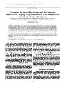
Since a city might include natural gaps, such as the River Thames in London or other topographic obstacles, it is convenient to define cities as connected clusters of neighboring populated sites. This idea has been recently implemented in the so called City Clustering Algorithm (CCA) [24], which is an adapted version of the more general Burning Algorithm [34]. Basically, CCA identifies any pair of adjacent urban spatial units (either by population or land cover) as belonging to the same urban cluster if these are located within a distance l from each other. Thus, when applied to an entire region, CCA provides a mean to determine the areas and boundaries of the cities contained within, according to the parameter l, which represents a degree of coarse-graining. At the global scale, data on the spatial distribution of population is only available for administrative boundaries or as raster data with a rather coarse resolution. Therefore, we opted for determining the area of cities a remote sensing based classification of land cover data, as provided by the GlobCover 2009 land cover map [15] at a grid resolution of approx. 0.308 km (at the Equator). From the 23 land cover classes, we selected and aggregated those corresponding to urban land use. For the sake of illustration, Fig. 1 exhibits the application of the CCA to the land cover data for Paris and its surroundings. A satellite image of the region is displayed in Fig. 1(a), the corresponding aggregated land cover classes in Fig. 1(b), and the urban clusters identified after application of the CCA in panel Fig. 1(c). Since the raster cell size decreases from the Equator to the poles, the use of the Euclidian metric is not suitable for the application of CCA at the global scale. Accordingly, orthodromic distances were considered in a new implementation of the CCA in order to provide a more accurate representation of distances and areas across different latitudes on a sphere. In the orthodromic representation, a distance determined in terms of the latitude yi and longitude xi coordinates is given by di,j = REarth cos−1 (ψi,j ) where ψi,j = (sin(xi ) sin(xj ) + cos(xi ) cos(xj ) cos(yi − yj )) with the radius of the terrestrial sphere REarth ≈ 6.371 × 103 km.

III.

GLOBAL CITY SIZE DISTRIBUTION

With the aim of addressing the global city size distribution, we applied CCA with a clustering distance of l = 0.4km to the entire global land cover database referred to in Sec. II, from which we extracted 249, 512 urban clusters. The resulting area probability density p(A) is shown in Fig. 2(a). Besides deviations for small sizes – which are mainly due to the discreteness of the grid cells – we find a fair power-law relation in agreement with Eq. (1), with X = A and ζA ≈ 1.93 for A ≥ 1 km2 .

In terms of population, the global probability density, was obtained using population data from the Global Rural Urban Mapping Project (GRUMP) [10], which comprises coordinates, names, and population figures of 67, 935 administrative units (estimated data for the year 2000). From this sample we found 16, 908 urban settlement points which are located inside an urban cluster or within a distance of l = 0.4 km (following a similar approach as in [25]). Figure 2(b) shows the population probability density p(S). Since, the number of small clusters which could be assigned to a cluster and accordingly to a number of inhabitants is small, we observe in Fig. 2(b) deviation from the power law distribution Eq. (1) at the lower end. Therefore, the power law fitting is carried out for urban clusters above 104 inhabitants, resulting in an exponent ζS = 1.85. Accordingly, we observe that Zipf’s law approximately holds for the cities on the global scale, whereas the actual exponent is smaller than 2. We explore also l = 4 km and similar power-law size distributions, however with a different exponent in the case of the areas (Fig. 2(a)). Studies of global population city size distributions were reported in [4, 38], for a reduced subset of cities, e.g. the 2, 700 largest clusters in the case of the former. Distributions of city size in terms of area has been considered previously, e.g. in [1, 17, 19, 25, 29] at the regional and country scale. More recently, a global analysis has positively tested Zipf’s law by considering temporally stable night lights as a proxy indicator for human habitation and anthropogenic land use [31].

IV. PERCOLATION TRANSITION AND SIZE DISTRIBUTION ON THE COUNTRY SCALE A.

Percolation transition

It is worth noting that when the clustering parameter l is set to a very small value the CCA does not take any effect, in the sense that the urban clusters thereby identified correspond trivially to those observed from the input land cover map. On the other hand, in the opposite limit of very large l, most of the urban area under scope are assigned to a same giant cluster component. Accordingly, when applied to a large area, for intermediate values of l it is expectable to observe a percolation transition of the urban clusters. As it turns out, it becomes natural to inquire into this possibility and to eventually address the spatial properties drawn from application of the CCA in the light of concepts and methods stemming from percolation theory [9, 34]. At the country scale, let us address the possible percolation transition that may occur at the level of the urban patch clustering when changing the parameter l in a typical application of the CCA – which, more in general, constitutes a problem inherent to the ambiguous character of the definition of city boundaries [1, 6, 24]. It is in order to mention that the scale defined by the clustering

3 parameter l determines the type of percolation transition under scope – for small l, the transition resembles the one occurring in site percolation on a square lattice, while for large l it can be further assimilated to the one observed in continuum percolation problems [9]. Here, we are interested in the value lc at which the giant cluster component spans within a country territory. The critical value lc is analogous to the critical occupation probability Pc , which constitutes the control parameter in most of lattice percolation formulations [9]. Both quantities are approximately related by P ∼ lβ with β ≈ 2. In real world data, however, it can be difficult to identify such an lc percolation threshold. We find that the average cluster size excluding the largest cluster, hAi∗ , constitutes a sensitive indicator of the transition. In infinite systems, hAi∗ diverges at Pc [9] – in case of finite systems a (finite) peak occurs. Similarly, one can in principle detect the presence of a peak in hAi∗ around a value lc when applying CCA to the urban land cover of different countries. Since in the limit of small l the urban clusters identified by the CCA approximate the cells of urban land cover, we conjecture that a small lc value constitutes a proxy indicator of the percolation threshold of the urban land cover. For illustrative purposes, let us consider the case of Austria. Figure 3(a) depicts the plot of hAi∗ vs. l. As it can be observed, for l < lc the average cluster size increases strongly with l, yet gradually, and it drops sharply for l > lc . In the case of Austria we find that the peak occurs at lc = 15 km. In a model based on correlated percolation [19, 20] the urban/non-urban structure is formed from spatial correlations, i.e. the probabilities of two sites being urban/non-urban are more similar the closer they are. Furthermore, a radial decay of density around the city center is assumed. A similar approach has been recently applied to reproduce the scaling properties observed in urban land parcels [8]. The dynamics and characteristics of the percolation transition of the urban land cover has been investigated also by means of diffusion limited [21] and gravity based [27] stochastic aggregation models of city growth.

B.

City size distribution

Let us now consider the influence of the coarse-graining used in defining a city cluster, i.e. parameter l in the CCA, on the scaling of the city size distributions. At this stage, we stress the fact that for many countries lc cannot be identified unambiguously (see e.g. inset of Fig.5(b)), as for instance in the presence of multiple peaks – often a signature of large clusters being disconnected by vastly extended topographic heterogeneities. Therefore, we focus on a selected set of countries exhibiting (i) a clear percolation threshold and (ii) a large number of urban areas. For a given l value we extract all city cluster areas Ai

and estimate the corresponding exponent ζA by applying the method proposed in [11] and testing power-law against log-normal. Thus, we first quantify the pointwise log-likelihood ratios between the fitted power-law and fitted log-normal distributions and then apply the Voung test for non-nested models [36]. This test essentially consists in testing the hypothesis that both distributions are equally far away from the true distribution, against the two alternative cases where either of each distributions is closer to the true distribution than the other one. Consequently, we account only for those cases where the fitted ζA -values results in positive Voung test and where the associated one-sided p-value exceeded 0.9 (which corresponds to a significance level of 10%). For this procedure we used the corresponding R code (available at http:// tuvalu.santafe.edu/~aaronc/powerlaws/). We vary l and repeat the procedure to obtain ζ(l). Figure 3(b) shows the probability density p(A), as obtained for the same country as in Fig. 3(a) for two different values of l (for illustrative purposes, normalized histograms with logarithmic binning are shown). The fitting results in ζA = 1.71 and ζA = 1.27, for l = 5 km and l = 10 km, respectively. Similar decreases in ζ are also found for other countries (see Fig. 3(c)). From these fndings, we conjecture an approximately logarithmic dependence on the ratio l/lc , with ζA ≈ 2 for l  lc and ζA ≈ 3/2 . . . 1 for l → lc . We cannot determine the exact value for l → lc , since the sample sizes become small and the estimated ζ unreliable. Note that the curves in Fig. 3(c) do not fully collapse, in the sense of [33], i.e. the curves do not fall on the identical line, from which we learn that there must be other influences beyond our analysis, such as heterogeneities in the urban land cover. Another possible explanation for this could be measurement errors in the estimation of ζA and lc . We stress the fact that the size distributions of urban land cover clusters appear to agree with the functional form in Eq. (1), independently of the distance to the percolation threshold lc – in contrast to the case of uncorrelated percolation where a power-law size distribution of clusters emerges only in the close vicinity of the transition threshold [9]. Decreasing ζ with increasing l has also been reported for the USA [25]. Moreover, a recent study of a “gravity” based urban growth model [27] has shown that ζ(P ) ≈ a + b ln(P ) + c ln(1 − P ), where P represents the site occupation probability. Depending on the values of a, b, and c, this expression leads to a similar decay as in Fig. 3(c). This similarity suggests a generic influence of the proximity to the percolation threshold on the powerlaw size distribution of urban land cover.

C.

Average size scaling

According to percolation theory, the average cluster size of finite clusters, hAi∗ , i.e. disregarding the largest cluster, scales with the proximity of the occupation probability to the critical probability, hAi∗ ∼ |P − Pc |−γ ,

4 where the exponent γ is universal and only depends on the dimension [9]. It is of our interest to explore whether the percolation of the urban land cover clustering exhibits a similar scaling. Since in our analysis only few clusters remain above the percolation transition, we omit the case l > lc and study hAi∗ as a function of (lc − l). Figure 4 shows the results for Austria and Denmark. Due to the finite size of the countries, hAi∗ does not diverge for (lc − l) → 0 and we see a plateau. In the other limit, hAi∗ → 1 for large l → 1. In between we find a regime approximately following a power-law hAi∗ ∼ (lc − l)−γ .

(2)

In general, we did not find a universal behavior as in random percolation, in the sense that the values obtained for γ can strongly differ among countries. For instance, for Austria, least squares fitting provides γ ≈ 2 and for Denmark γ ≈ 1.25. Such a variability in the γ values can result from measurement errors in the identification of lc (as discussed in Sec. IV A) or due to systematic structural influences occurring at larger scale, such as the presence of spatial correlations or an accidented topography. Moreover, in some countries the plot of hAi∗ vs. l does not exhibit a clear power law relation. On one hand, the log-log plot of hAi∗ vs l can appear as composed by many linear segments, or, furthermore, the presence of a power-law-like segment cannot even be adequately prescribed over a substantial range of l-values.

D.

Taylor’s law for city size distribution

Beyond the behavior of the average size with l, characterizing the scaling properties of urban clusters requires also to attend to statistical regularities occurring at the level of the variability of the cluster sizes. For this purpose we elaborate on an empirical relation first established in the context of ecology, the so called Taylor’s law [32, 35]. In systems satisfying Taylor’s law, the standard deviation and the average of a quantity are related by a power-law. Both quantities are either temporal or over ensembles. According to [12], in the case of temporal variability it follows either a linear or square-root scaling. For a recent review on this topic we refer to [14]. In the case of cities, we consider the standard devia∗ tions and average of cluster sizes for a given l, i.e. σA (l) ∗ and hAi (l), whereas we omit the largest cluster (this is necessary since at least for l > lc it is an outlier). By varying l, the ensemble of cluster sizes and the hypothesized power-law can be investigated. ∗ σA ∼ (hAi∗ )α

(3)

In Fig. 5 we show the results for two example countries ∗ (Austria and Spain). While the major panels display σA ∗ vs. hAi , the corresponding l can be inferred from the color-coded insets. For Austria (Fig. 5(a)), a power-law regime is found for small l, i.e. l ≤ 10 km with α ≈ 0.79.

The slope seems to hold up to l ≈ 15 km but separated by jumps in the standard deviation. In contrast, for Spain (Fig. 5(b)), two different power-law regimes can be seen, the first up to l ≈ 4 km with α1 ≈ 1.63 and the second one up to l ≈ 16 km with α2 ≈ 0.76. For other countries we obtained similar results. We conclude that Taylor’s law holds to some extent for city sizes but there is no unique exponent and the scaling regimes are country specific. Nevertheless, we ∗ observe a characteristic maximum in the plot of σA vs. ∗ hAi . In the case of Austria, this maximum matches with the percolation threshold lc . In the case of Spain, the maximum standard deviation is located at the similar position as a small peak in the representation of hAi∗ vs. l (inset of Fig. 5(b)). This suggests a relation between the percolation threshold lc and Taylor’s law, where the presence of a maximum of the latter could constitute a mean to identify the former. E.

Spatial correlations

In the context of the analysis of the scaling properties of city clusters, it is worth stressing the role dynamic processes underlying city growth play. As shown in [19, 20], city cluster size distributions are influenced by the presence of spatial correlations. The above mentioned gravity based model of urban growth [27] has illustrated the relation between the degree of compactness of urban clusters and the exponent ζ of the cluster size distribution Eq. (1). With the aim of addressing the spatial organization of real urban clusters we calculate the auto-covariance function C(d) = h(xi − hxi)(xj − hxi)|dii,j ,

(4)

Here, xi , xj represent the land cover of sites i, j, respectively, i.e. x = 1 for urban and x = 0 otherwise. The indices i, j run over all land cells and the average (denoted by brackets) is taken on those cells lying within a distance d, which is predefined by logarithmic bins. In Fig. 6 we show C(d) for Austria and the Netherlands as illustrative cases. As can be observed, C(d) remains positive for scales at least up 100 km and it decays with distance, approximately following a power-law C(d) ∼ d−ξ .

(5)

Note however that at large distances, the decay exhibits a cut-off where C(d) drops considerably. In order to take the cut-off into account, we elaborate further on the fit C(d) ∼ e−λd d−ξ

0

(6)

as used e.g. by [11] in different contexts. We fit Eq. (5) to the approximately linear regime of ln C vs. ln d by means of least squares and Eq. (6) by employing non-linear curve-fitting applying the GaussNewton-Algorithm (cf. [3]). While both approaches,

5 Eq. (5) and Eq. (6), lead to different exponents ξ and ξ 0 , these are both lower than 2, thereby indicating the presence of long-range correlations. Regarding the relation between the correlation decay and the percolation threshold, it has been shown that long-range correlations can influence the percolation properties [37]. However, according with [23], the influence of correlations on the threshold value is only minor. For instance, for site percolation on a square lattice [23], the site occupation probability threshold has been shown to vary slightly between Pc ' 0.593 for the case of no long-range correlation effect (ξ = 2 in Eq. (5)) and Pc → ≈ 0.5 for the case of strong long-range correlations (ξ = 0 in Eq. (5)). As mentioned in Sec. IV B, spatial inhomogeneities can hinder unambiguous identification of the clustering threshold lc . Since long-range spatial correlations can entail spatial inhomogeneities, quantification the weak influence of correlations on the value of lc cannot be achieved in many cases.

V.

CITY ALLOMETRY – RELATING AREA AND POPULATION

An important aspect in the analysis of cities is their allometry properties, i.e. the relation between the city sizes (e.g. given by population) and their socio-economic “functions” [7] and structure. Of particular interest in this context is the relation between city size and area [5]. Thus, we last address the relation between urban cluster population and area. For this purpose, we combine urban land cover data, as provided by GlobCover, with the pointwise population numbers of the 67, 935 administrative cities included in the GRUMP database. We match population and area of clusters by summing up for each cluster those population numbers, that are located within the distance l to the considered cluster (similar to the procedure followed in [25]). Figure 7(a) depicts the obtained relation between area and population. Most clusters are spread around S ∼ Aδ , except clusters with small population which exhibit discreteness (stemming from the land cover resolution) and deviate from the power-law. In order to overcome this difficulty, we remove a fraction q of clusters for both, S and A low values, as indicated by blue lines in Fig. 7(a). It is also necessary to consider that a direct fitting of log(A) vs. log(S) and log(S) vs. log(A) statistically leads to different results. Therefore, we assimilate δ to the slope of the longitudinal principal axis of rotation of the cloud of points in the log(A) vs. log(S) plot, as obtained from the eigenvector analysis of the corresponding tensor of “inertia”. In order to address the dependency of the correlations between area and population on the observational scale, i.e. on the clustering parameter, in Fig. 7(b) we plot for q = 0.2 the Pearson correlation values as a function of l and consistently find values above 0.85 with a maximum of approx. 0.88 at approx. 5 km. Figure 7(b) also shows

the values of δ. For very small l, highest values are found between δ ≈ 0.85 for q = 0.2 and δ ≈ 0.93 for q = 0.4. For other values of l, the slope fluctuates but generally δ is roughly within 0.82 and 0.87. As it turns out, the results show a sublinear population to area relation, i.e. δ < 1. In other words, we find that for a given increase in population, the associated increase in area is greater for large cities than for small ones. While [5] suggests an evolution of δ, i.e. that estimations of δ are decreasing since the 1940s, our results indicate an l-dependence of δ, i.e. that the value depends on the observational scale, but generally in the lower range of those listed in [5]. This is a relevant fact, since, as before mentioned, allometry could be responsible for the scaling of socio-economic quantities with the population of cities, including urban CO2 -emissions [22, 28].

VI.

SUMMARY AND DISCUSSION

In this paper we have elaborated on the influence exerted by the degree of coarsening resolution that is inherent to the definition of city boundaries, on a set of indicators of the scaling, spatial organization, and allometry aspects of urban clusters. For this purpose we implemented a version of the City Clustering Algorithm that takes the curvature of the globe into account and apply it to global satellite based information on the global urban land cover, in combination with pointwise information of populated units worldwide. Our results show that, at the global scale, Zipf’s law is found to approximately hold to a great extent for the areas of urban clusters and to a lesser extent for the corresponding population. A shortcoming is the error introduced by automatized identification of urban areas from satellite imagines as inherent in the land cover data used in this study. As a matter of fact, the climatological, vegetational and structural variety of urban clusters on the globe can hinder their classification, e.g. in GlobCover data Kabul city is not classified as urban. For a recent alternative analysis of size distributions of city clusters on the global scale we refer to [18]. At the country scale, we addressed the percolation transition that may occur, at the level of the urban cluster definition, when coarsening the resolution considered to identify urban clusters. This information is relevant as a proxy indicator for detecting the proximity to the percolation transition occurring eventually on the real land cover of large urbanized areas – which in turn could exert influence on important factors of the sustainability, such as Urban Heat Island effect (see e.g. [39]), landscape fragmentation, water surface run-off and floods control, among others. As a matter, identifying an urban clustering percolation threshold can become a cumbersome task, due, for instance, to spatial inhomogeneities in the distribution of urban clusters at the large country scale. In this work we used as an indicator the behavior of the average cluster size, excluding the largest one, which

6 itself provides a suitable characterization of urban clusters, for different levels of coarsening-resolution. This analysis was applied to selected country cases, for which we addressed the linkage between the scaling of urban cluster sizes and the degree of resolution used for their definition. Our results appear to be at a certain degree consistent with recent results obtained numerically in a simple gravity-based urban growth model. Beyond the scaling and average size, characterization of urban clusters requires addressing the scaling of deviations of cluster sizes around the average. In particular, for the selected country cases, we illustrate the validity of Taylor’s law between average urban cluster sizes and their standard deviations. Moreover, we show that strong deviations from Taylor’s law can be readily used to identify threshold values in proxy indicators of the percolation transition of urban clustering, in cases where the average cluster size fails. Regarding the spatial organization of urban clusters in selected country cases, we find the presence of long-range correlations decaying as a power law with exponential cut-off. However, for densely urbanized areas we find that a power-law decay is further significative, as compared to

the fitting of a power-law with exponential cut off. Finally, our results on the relation of area to population indicate that for a given increase in population, the associated increase in area is greater for large cities than for small ones. A shortcoming in our analysis of city allometry is the minor time period discrepancy between the population and land cover databases – that actually represent the most updated and accurate publicly available global databases.

[1] Arcaute, E., Hatna, E., Ferguson, P., Youn, H., Johansson, A., Batty, M., 2013. City boundaries and the universality of scaling laws. URL http://arxiv.org/abs/1301.1674 [2] Auerbach, F., 1913. Das gesetz der bev¨ olkerungskonzentration. Petermanns Geogr. Mitteilungen 59 (74), 73–76. [3] Bates, D. M., DebRoy, S., ???? R-Documentation: Nonlinear Least Squares. URL http://stat.ethz.ch/R-manual/R-patched/ library/stats/html/nls.html [4] Batty, M., 2008. The size, scale, and shape of cities. Science 319 (5864), 769–771. [5] Batty, M., 2011. Defining city size. Environ. Plan. BPlan. Des. 38 (5), 753–756. [6] Berry, B. J. L., Okulicz-Kozaryn, A., 2012. The city size distribution debate: Resolution for US urban regions and megalopolitan areas. Cities 29 (SI1), S17–S23. [7] Bettencourt, L., West, G., 2010. A unified theory of urban living. Nature 467 (7318), 912–913. [8] Bitner, A., Holyst, R., Fialkowski, M., 2009. From complex structures to complex processes: Percolation theory applied to the formation of a city. Phys. Rev. E 80 (3), 037102. [9] Bunde, A., Havlin, S. (Eds.), 1991. Fractals and Disordered Systems. Springer-Verlag, New York. [10] Center for International Earth Science Information Network (CIESIN), Columbia University; International Food Policy Research Institute (IFPRI), The World Bank; and Centro Internacional de Agricultura Tropical (CIAT), 2011. Global rural-urban mapping project, version 1 (grumpv1): Settlement points. Website, available at http://sedac.ciesin.columbia.edu/data/ dataset/grump-v1-settlement-points. Date of down-

load: 26.11.2011. [11] Clauset, A., Shalizi, C. R., Newman, M. E. J., 2009. Power-law distributions in empirical data. SIAM Rev. 51 (4), 661–703. [12] de Menezes, M. A., Barabasi, A. L., 2004. Fluctuations in network dynamics. Phys. Rev. Lett. 92 (2), 028701. [13] Eeckhout, J., 2004. Gibrat’s law for (all) cities. Am. Econ. Rev. 94 (5), 1429–1451. [14] Eisler, Z., Bartos, I., Kert´esz, J., 2008. Fluctuation scaling in complex systems: Taylor’s law and beyond. Adv. Phys. 57 (1), 89–142. [15] ESA (European Space Agency) 2010 The Ionia GlobCover project, ???? Globcover land cover 2009 v2.3. Website, available online at http://ionia1.esrin.esa. int; last accessed 21 August 2011. [16] Gibrat, R., 1931. Les in´egalit´es ´economiques. Libraire du Recueil Sierey, Paris. [17] Kinoshita, T., Kato, E., Iwao, K., Yamagata, Y., 2008. Investigating the rank-size relationship of urban areas using land cover maps. Geophys. Res. Lett. 35 (17), L17405. [18] Makse, H., ???? in preparation. [19] Makse, H. A., Andrade, J. S., Batty, M., Havlin, S., Stanley, H. E., 1998. Modeling urban growth patterns with correlated percolation. Phys. Rev. E 58 (6), 7054–7062. [20] Makse, H. A., S., H., Stanley, H. E., 1995. Modeling urban-growth patterns. Nature 377 (6550), 608–612. [21] Murcio, R., Sosa-Herrera, A., Rodriguez-Romo, S., 2013. Second-order metropolitan urban phase transitions. Chaos Solitons Fractals 48, 22–31. [22] Newman, P., Kenworthy, J. R., 1990. Cities and automobile dependence: an international sourcebook. Gower Publishing Company, Brookfield, VT, USA. [23] Prakash, S., Havlin, S., Schwartz, M., Stanley, H. E., 1992. Structural and dynamic properties of long-range

Acknowledgments

D. Rybski acknowledges E. Arcaute and A.P. Paolo Masucci for useful discussions. This work has been funded by the Federal Ministry of Education and Research (BMBF) through the program ”Spitzenforschung und Innovation in den Neuen L¨anden” (contract ”Potsdam Research Cluster for Georisk Analysis, Environmental Change and Sustainability” D.1.1) and partly by the RAMSES project of the European Commission under the 7th Framework Programme.

7

[24]

[25]

[26] [27]

[28]

[29]

[30] [31]

correlated percolation. Phys. Rev. A 46 (4), R1724– R1727. Rozenfeld, H. D., Rybski, D., Andrade Jr., J. S., Batty, M., Stanley, H. E., Makse, H. A., 2008. Laws of population growth. Proc. Nat. Acad. Sci. U.S.A. 105 (48), 18702–18707. Rozenfeld, H. D., Rybski, D., Gabaix, X., Makse, H. A., 2011. The area and population of cities: New insights from a different perspective on cities. Am. Econ. Rev. 101 (5), 2205–2225. Rybski, D., 2013. Auerbach’s legacy. Environ. Plan. A 45 (6), 1266–1268. Rybski, D., Garcia Cantu Ros, A., Kropp, J. P., 2013. Distance weighted city growth. Phys. Rev. E 87 (4), 042114. Rybski, D., Sterzel, T., Reusser, D. E., Fichtner, C., Kropp, J. P., 2013. Cities as nuclei of sustainability? online-arXiv arXiv:1304.4406 [physics.soc-ph]. Schweitzer, F., Steinbrink, J., 1998. Estimation of megacity growth – simple rules versus complex phenomena. Applied Geography 18 (1), 69–81. Simon, H. A., 1955. On a class of skew distribution functions. Biometrika 42 (3/4), 425–440. Small, C., Elvidge, C. D., Balk, D., Montgomery, M., 2011. Spatial scaling of stable night lights. Remote Sens. Environ. 115 (2), 269–280.

[32] Smith, H. F., 1938. An empirical law describing heterogeneity in the yields of agricultural crops, part: 1. J. Agric. Sci. 28, 1–23. [33] Stanley, H. E., 1999. Scaling, universality, and renormalization: Three pillars of modern critical phenomena. Rev. Mod. Phys. 71 (2), S358–S366. [34] Stauffer, D., Aharony, A., 1994. Introduction To Percolation Theory. Taylor & Francis, London, Philadelphia. [35] Taylor, L. R., 1961. Aggregation, variance and mean. Nature 189 (476), 732–735. [36] Vuong, Q. H., 1989. Likelihood ratio tests for model selection and non-nested hypotheses. Econometrica 57 (2), 307–333. [37] Weinrib, A., 1984. Long-range correlated percolation. Phys. Rev. B 29 (1), 387–395. [38] Zanette, D. H., Manrubia, S. C., 1997. Role of intermittency in urban development: A model of large-scale city formation. Phys. Rev. Lett. 79 (3), 523–526. [39] Zhou, B., Rybski, D., Kropp, J. P., 2013. On the statistics of urban heat island intensity. Geophys. Res. Lett. 40 (20), 5486–5491. [40] Zipf, G. K., 2012. Human Behavior and the Principle of Least Effort: An Introduction to Human Ecology (Reprint of 1949 Edition). Martino Publishing, Manfield Centre, CT.

8

100

FIG. 1: Application of city clustering to urban land cover data. The following panels illustrate different aspects of the city of Paris and its surroundings: (a) Remote sensing image as extracted from the ArcGIS 10 component ArcMap. (b) Urban land cover data as obtained from the GlobCover 2009 land cover map. The colors indicate urban (red, class 190), water bodies (blue, class 210), forests and grasslands (green, classes 20-110), and rainfield croplands (yellow, class 14). (c) From the urban land cover and by taking l = 4 km, the identified clusters are color coded according to the logarithm of their size: from small (light blue) via medium (green) to large (red). The cutout has the approximate area of (215 km)2 .

(a)

10−2

● ●

●

(b)

● ●

● ● ● ●

●

●

10−4

● ●

● ●

●●

●

● ●

●

●

P 10−6

● ●

●

●● ●

● ●

●

●● ● ●

●

●

●

● ●

●

●

●

●

●

●

10−8

●

● ●

●

●

● ●

10−12 10−10

● ●

●

●

●

● ●

●

●

400 m 4 km

10

−1

●

10

0

101 2

A [km ]

2

10

3

10

10

0

400 m 4 km

10

1

● ●

●

10

2

3

10

10 S

4

10

5

6

10

7

10

FIG. 2: Probability density of city size in terms of area and population. (a) Cluster area distribution p(A), as obtained by applying the City Clustering Algorithm (CCA) to global land cover data and extracting all urban clusters on the globe. For A > 0.1 km2 we estimate ζA ≈ 1.93 for l = 0.4 km (249,512 clusters) and ζA ≈ 1.75 for l = 4 km (46,754 clusters). (b) Cluster population distribution p(S), as obtained from associating population settlement points with the urban clusters identified by means of CCA. For S > 104 we estimate ζS ≈ 1.85 for l = 0.4 km and ζS ≈ 1.75 for l = 4 km. In both panels: l = 0.4 km (circles), l = 4 km (squares). The solid grey lines have slope −2.

100

9 (b)

0

10−8

5

* [km2] 10 15

p(A) [arb. units] 10−6 10−4 10−2

20

(a)

0

5

10

15

20 25 l [km]

30

35

10−2

40

●

10−1

100 101 A [km2]

102

103

2.5

●

(c) ● ● ●

● ●

● ● ● ●

● ● ● ● ● ● ● ● ● ● ● ●● ● ● ● ● ● ● ● ● ● ● ●●● ● ● ● ●● ● ● ● ● ● ●● ● ● ● ● ●● ● ● ●● ● ● ●● ● ● ● ● ● ●● ● ● ● ● ●● ● ● ● ● ● ●●●●● ● ●●●● ● ●● ● ●● ● ●● ●●●● ● ●● ●● ●● ● ● ● ● ● ● ● ●●● ●● ● ● ● ● ● ●●● ● ● ● ● ●● ●● ● ● ●●●● ● ● ● ● ● ● ●●● ●● ● ●● ●● ● ● ●● ● ● ● ● ● ● ● ●●●● ● ●● ● ● ●● ● ●● ● ● ● ● ●● ● ●● ●● ● ●● ● ● ●●●● ● ● ● ● ● ●● ● ●●● ●●● ●●●●●● ● ●● ●●● ●●● ●● ● ● ● ● ● ● ●● ● ● ●● ● ● ●● ● ● ● ●●● ●●●● ●● ●● ● ● ●● ●● ●● ● ● ●● ● ●● ● ● ● ● ● ● ●●● ● ● ●●● ●● ● ● ●●● ●● ● ● ● ● ● ● ●●● ● ● ● ●● ● ●● ● ●● ●●●●● ● ● ● ●● ● ● ●●● ● ●●● ● ●● ● ● ●● ● ● ● ● ● ● ● ● ●● ●● ●● ● ● ●● ● ●● ● ● ● ● ● ●● ● ●● ● ● ●● ● ● ●●● ● ● ● ● ● ● ● ● ● ● ● ● ● ●●● ● ● ● ●● ●● ●● ● ● ● ● ● ●● ● ● ●●● ●● ●● ● ● ● ● ● ● ● ● ● ● ● ● ● ●● ● ● ●● ●

● ● ● ● ●

● ●●

● ●

●

●

●

●

●

●

● ●

● ●

1

ζ 1.5

2

Austria Poland Belgium Denmark Finland Portugal France Romania Spain Netherlands Switzerland Italia

●

0.5

●

10−4

10−3

10−2

l lic

10−1

100

101

FIG. 3: Percolation and Zipf’s law. (a) Average cluster size excluding the largest component hAi∗ as a function of the clustering parameter l for Austria. The maximum is located at the percolation transition, which in this example is lc ' 15 km. (b) Probability density of cluster areas p(A) for Austria and for l ' 13 lc (370 clusters, green triangles) as well as l ' 32 lc (87 clusters, brown squares). The dotted grey lines have the slopes −1.71 and −1.27. (c) Estimated power-law distribution exponent ζA as a function of the rescaled clustering parameter l/lc for various countries as indicated by colored dots. Since we found out that the method proposed in [11] has a significant deviation from the real value for input with less than 100 entries, we estimated the power-law distribution exponents for each country just for those l with at least 100 clusters remaining. The open circles represent averages in logarithmic bins and their error bars the corresponding standard deviations. The exponent decreases with increasing l/lc and takes values between ζA ≈ 2 for l/lc  1 and ζA ≈ 3/2 . . . 1 for l/lc → 1.

(a) ● ● ●

* [km2] 100

●

●●●●●● ● ● ●● ●● ●● ●●● ●● ● ● ● ● ● ● ● ● ● ● ● ● ● ● ● ● ● ● ● ● ● ● ● ● ● ● ● ● ● ● ● ● ● ● ● ● ● ● ● ● ● ● ● ● ● ● ● ● ●

10−1

●

●

●

● ● ● ● ● ● ● ● ●●●

●

101

●

(b)

● ●● ●● ● ●● ●● ● ●● ●● ● ● ● ● ● ● ● ● ● ● ● ● ● ● ● ● ● ● ● ● ● ● ● ● ● ● ● ● ● ● ● ● ● ● ● ● ● ● ● ● ●

100

●

101

●

102

102

10

●

10−1

10−2

●

10−1

100

101

lc − l [km]

102 10−1

100

lc − l [km]

101

102

102

101

FIG. 4: Fitting of the average size scaling for Austria (a) and Denmark (b). In both cases we have a unique clear peak in the curve of hAi∗ against l. The red lines represent the fittings of the function f (x) = c · xa on the green highlighted parts. Fittings yields the parameter a ≈ −1.9674 for Austria and a = −1.2519 for Denmark.

(b) ●

●● ●● ● ●●● ●●● ● ●● ●● ●● ●● ● ● ● ● ● ● ● ● ●● ● ● ● ●● ● ●● ● ● ●●●●●● ●● ●●● ● ● ● ● ● ●● ● ● ●● ● ● ●● ● ● ●●● ●● ●●● ● ●● ● ● ●●● ●● ● ● ● ● ● ● ● ●● ● ● ● ● ● ● ● ● ● ● ● ● ● ● ● ● ● ● ● ● ● ● ● ● ● ● ● ● ● ● ● ● ● ● ● ● ● ● ● ● ● ● ● ● ● ● ● ● ● ● ● ● ● ● ● ● ● ● ● ● ● ● ● ● ● ● ● ● ● ● ● ● ● ● ● ● ● ● ● ● ● ● ● ● ● ● ● ● ● ● ● ● ● ● ● ● ● ● ● ● ● ● ● ● ● ● ● ● ● ● ● ● ● ● ● ● ● ● ● ● ● ● ● ● ● ● ● ● ● ● ● ● ● ● ● ● ● ● ● ● ● ● ● ● ● ● ● ● ● ●

●● ●●●● ●

σ* 100

●

● ● ●

10

10−1

● ● ● ● ● ● ● ● ● ● ● ● ● ● ● ● ● ● ● ● ● ● ● ● ● ● ● ● ● ● ● ● ● ● ● ● ● ● ● ● ● ● ● ● ● ● ● ● ● ● ● ● ● ● ● ● ● ● ● ● ● ● ● ● ● ● ● ●

0

● ● ●

−1

●

● ● ● ●

0

* [km2]

● ● ● ● ●

10 20 l [km]

10

1

● ● ●

● ● ● ● ● ● ● ● ● ● ● ● ● ● ● ● ● ● ● ● ● ● ● ● ● ● ● ● ● ● ● ● ● ● ● ● ● ● ● ● ● ● ● ● ● ● ● ● ● ● ● ● ● ● ● ● ● ● ● ● ● ● ● ● ● ● ● ● ● ● ● ● ● ●

0

● ●

0

●● ●● ●● ●● ●● ●● ●● ●● ● ●● ●● ● ● ● ●● ●● ● ● ● ●● ● ● ● ● ●

5

* [km2] 10 15 20

●

●●

10

120

● ● ● ● ● ● ●● ● ● ●●

101

●

30

● ● ● ● ● ● ● ● ● ● ● ● ● ● ● ● ● ● ● ● ● ● ● ● ● ● ● ● ● ● ●● ● ● ● ● ● ● ● ● ● ● ● ● ● ●●● ● ● ● ● ● ● ● ● ● ● ● ● ● ● ● ● ● ● ● ● ● ● ● ● ● ● ● ● ● ● ● ● ● ● ● ● ● ● ● ● ●

0 2

10

10

−1

0

10

1

100

● ● ● ● ●

● ●●●

10 * [km2]

20

40 60 l [km]

10

2

80

10−1

●● ●

● ●

* [km2] 40 80

(a)

103

FIG. 5: Taylor’s law for city sizes. The standard deviation ∗ of cluster sizes disregarding the largest cluster is plotted as σA a function of hAi∗ for various values of l. The panels show the results for (a) Austria and (b) Spain. The insets depict the corresponding curve of hAi∗ against l (see also Fig. 3(a)). In the panels and insets corresponding coloring is used in order to enable comparison. For Austria, the standard deviation ∗ σA reaches its maximum at l = 15 km (light-blue) and for Spain it is located at l = 13.6 km (yellow). In the former case this maximum corresponds to the percolation point. In the latter case the maximum corresponds to the first peak one can identify in the curve of hAi∗ against l.

●

(a)

● ● ● ● ● ●

● ● ● ● ●

(b)

● ●

● ● ● ●

●

● ● ● ●

● ●

● ●

● ●

● ●

● ● ● ● ● ●

● ●

● ●

● ●

● ●

10−3

● ●

● ● ● ●

● ●

● ●

● ●

● ● ● ●

● ●

● ● ● ●

C(d)

10−1

● ●

10−2

10−2

11

● ● ● ●

● ●

● ●

● ●

● ● ● ●

● ●

10−3

10−4

● ● ● ● ● ●

● ●

● ●

●

10

10

3

4

d [m]

10

10−4

10−5

● ●

2

5

10

10

2

10

3

4

d [m]

105

10

●

δ (q=0.2) C (q=0.2)

● ●

0.95

●

●

δ (q=0.3) δ (q=0.4)

0.90

(b)

(a)

2

3

FIG. 6: Spatial correlation computations for Austria (a) and Netherlands (b). The fitted curve (red) on the greenhighlighted points which follows the function f (x) := c · xa · exp(b · x) (power-law with exponential cut-off) has the values for Austria (a, b, c) ≈ (−0.177, −1.866 ∗ 10−4 , 0.013) and for the Netherlands (a, b, c) ≈ (−0.647, −1.052 × 10−5 , 2.021). The grey lines (fitted on the corresponding points below the displayed part) has slopes ≈ −0.4615 for Austria and ≈ −0.7331 for the Netherlands. Above the shown range, C(d) fluctuates around zero.

● ● ● ●●

● ●

●

●

−3

0.70

−2

0.75

0.80

●

●●●●● ●●●●● ● ●● ●● ●●●●●●● ●●●●● ●●●●●●●● ● ● ●● ●● ● ●●●● ● ●●●● ●●●●●●● ● ●● ●●●●●●●● ●●● ●● ● ●●●●● ●●●●●●●●●●●●●● ● ●● ●● ●●● ●● ●●●● ●●●●●●●●● ● ● ● ●●● ●●●● ●●●●● ● ●● ●● ● ●●● ●● ● ●●●●●●●● ●

●

0.85

log(S) − log(SCM) −1 0 1

●

−2

−1 0 1 2 log(A) − log(ACM) [log(km2)]

0

5 l [km]

10

FIG. 7: Correlations between area and population. (a) log(S) vs. log(A) for l = 0.4 km and of all land cover clusters that could be matched with population figures (grey dots). The blue vertical and horizontal lines truncate the fraction q = 0.2 along both axis in order to avoid the discreteness at small A. The green solid line corresponds to the main axis around which the momentum of inertia of the truncated cloud is minimal. In this case, 8786 out of 12321 clusters remain. It’s slope δ is smaller than the diagonal (black dashed line, background). (b) Slope δ (circles) and Pearson correlation coefficients C (squares) vs. clustering parameter l for the cut-off q = 0.2 (green, red), q = 0.3 (magenta), q = 0.4 (orange). The exponent δ is found roughly between 0.82 and 0.87 except for small l where δ up to 0.87 and 0.93 are achieved but always below 1. For q = 0.2 the correlations exhibit a maximum around 5 km.