programs. There is a software tool under development based on gnu g++ compiler ... complexity of the data used and the complexity of data handling into ...
MATHEMATICAL i$iLPR MODELLING PERGAMON
Mathematical
and
Computer
Modelling
38 (2003)
815-827 www.elsevier.com/locate/mcm
The Structured Complexity of Object-Oriented Programs A. F~THI, J. NY~KY-GAIZLERAND
Z. PORKOLAB
Department Pazmany
of General Computer Science E6tv6s Lor&nd University Peter set&y l/D., H-1117 Budapest, Hungary Bludens.elte.hu
Abstract-There are several methods measuring the complexity of object-oriented programs. Most of them are based on some special object-oriented feature: number of methods/classes, cohesion of classes, inheritance, etc. In practice, however, object-oriented programs are constructed with the help of the same control structures as traditional ones. Moreover, recent ideas of multiparadigm programming (i.e., emerging use of generic programming and aspect-oriented programming) has the effect that in modern programs-and even in class libraries-object-orientation is only one (however major) construction tool among others. An adequate measure therefore should not be based on special features of one paradigm, but on basic language elements and construction rules which could be applied to many different paradigms. In our model discussed here, the complexity of a program is the sum of three components: the complexity of its control structure, the complexity of data types used, and the complexity of the data handling (i.e., the complexity of the connection between the control structure and the data types). We suggest a new complexity measure. First, we show that this measure works well on procedural programs, and then we extend it to object-oriented programs. There is a software tool under development based on gnu g++ compiler which computes our new measure. We can apply this tool to C and C++ sources to gain a number of quantitative results with our measure. @ 2003 Elsevier Ltd. All rights reserved.
Keywords-Software
metrics,
Object-oriented
programming,
Complexity
1. INTRODUCTION There are several methods of measuring program complexity. The complexity of programs depends on the number of operators and operands (the software science measure) and on the number of predicates (cyclomatic complexity). However, these measures do not characterize sufficiently the nature of complexity, since n nested loops or n nested if statements are undoubtedly more complex than the sequence of n loops, or the sequence of n decisions. The complexity of (procedural) programs was so far mostly measured either on the basis of its control structure or on the data they used [l]. Nowadays, one of the most frequently used ‘Lwords” in the literature of programming methodology is the ‘object-oriented’ one. While constructing great systems the questions of reusability and extendibility became of key importance. The simpler a program is, the easier it is to understand, later to modify or reuse some parts of it in the case of the construction of other similar
0895-7177/03/$ - see front doi: 10.1016/S0895-7177(03)00283-8
matter
@ 2003
Elsevier
Ltd.
All rights
reserved.
Typeset,
by &@-TEX
816
A. F~THI
et al
programs. Followers of object-oriented methodology state that professional software production becomes notably simplified using this new technique, which results in enormous cost decrease. Measuring object-oriented software is often based on special object-oriented notions. However, modern programming languages implement facilities not only for the object-oriented paradigm. These languages still have very strong procedural parts. Also, new emerging techniques, most cases orthogonal to object orientation, are used in cooperation with object theory. The C++ language is one of the most frequently used modern languages in Europe--uses generic programming techniques: templates, traits, iterators with cooperation of classes, inheritance, etc. [2]. SUN plans to invent templates for the Java language, too. Aspect-oriented programming [3] is another important technique from XEROX Palo Alto Research Center. Aspects are applied to object-oriented Java programs to reduce complexity, eliminating cross-cutting code segments. These paradigms are heavily mixed in recent programs [4,5]. Inheritance from a template class, generic algorithms receiving template parameters are everyday practices in C++, including the standard library. It seems illogical to measure such programs or libraries only from the point of one paradigm. An adequate measure, therefore, should not be based on special features of one paradigm, but on basic language elements and construction rules applied to different paradigms. Based on the previous works of Piwowarski [6], Harrison and Magel [7,8], and Howatt and Baker [9], we introduce a new measure of complexity. Our main proposal is that when counting the complexity of a program, we should take the complexity of the data used and the complexity of data handling into consideration; we should see the decreasing of complexity through hiding techniques. Accordingly, the complexity of a program depends on three components: (i) the complexity of its control structure, (ii) the complexity of data types used, and (iii) the complexity of the data handling (i.e., the complexity control structure and the data types).
of the connection
between the
We suggest a new measure of complexity of a program or (class) library. First, we show this measure working well on procedural programs. Then, we extend the measure to object-oriented programs in the following steps. (1) We define the complexity of class. Class is defined as a set of data (attributes) and control structures (member functions, methods) working on the attributes. We define the complexity of class as a sum of the complexity of attributes and the complexity of member functions. The definition reflects the common experience that good objectoriented programs have very strong bindings between the attributes and the methods inside the class and have weak connections between different classes. The measure is also examined on special cases, such as member functions calling other member functions, and classes with no attributes (old-style libraries), etc. (2) We examine the complexity issues of the connection of classes. Inheritance and aggregate relationships between classes can increase global complexity of the program. However, every time we use the same class we can see the benefit of these constructions. In some classical examples, we show how complexity depends on binding between classes.
2. PRELIMINARY
DEFINITIONS
AND
NOTIONS
a
We shall define the new measure on the basis of the definitions given to the complexity of nested control structures. The definitions connected to this come from the “rigorous” description of [9]. DEFINITION 1. A directed graph G = (N, E) consists of a set of nodes N and a set of edges E. An edge is an ordered pair of nodes (x, y) . If (CC,y) 1s . an edge then node x is an immediate predecessor
The Structured
817
Complexity
of node y and y js an immediate successor of node x. The set of all immediate predecessors of a node y is denoted IP(y) and the set of all immediate successors of a node x is denoted IS(x). A node has indegree n if E contains exactly n edges of the form (w, 2). Similarly, a node has outdegree m if E contains exactly m edges of the form (z, 20). DEFINITION
where Vi[l
2. A path P in a directed graph G = (N, E) is a sequence of edges
< i < lc] 3 (cc~,z~+I) E E. In this case, P is a path from ~1 to IIJ~.
3. A flowgraph G = (N, E, s, t) is a directed graph with a finite; nonempty nodes N, a finite, nonempty set of edges E, s E N is the start node, t E N is the terminal For any Aowgraph G, the s start node is the unique node with indegree zero; the t terminal is the unique node with outdegree zero, and each node x E N lies on some path in G from Let N’ denote the set N - {s, t}.
DEFINITION
Howatt
set of node. node s to t.
and Baker define the notion of the basic block for modeling control flow as follows.
4. A basic block is a sequential block of code with maximal length, where a sequential block of code in a source program P is a sequence of tokens in P that is executed starting only with the first token in the sequence, all the tokens in the sequence are always executed sequentially, and the sequence is always exited at the end. Namely, it does not contain any loops or if statements.
DEFINITION
DEFINITION
5. Every node n E N of a Aowgraph G = (N, E, s, t), which has outdegree greater
than one, is a predicate node. Let Q denote the set of predicate nodes in G. The well-known measure of McCabe (cyclomatic complexity) is based only on the number of predicates in a program: V(G) = p + 1. The inadequacy of the measure becomes clear, if we realize that the complexity depends basically on the nesting level of the predicate nodes. The measures proposed in [6-81, proven to be equivalent in principle (see [9]), take this lack into account. 6. Given a Aowgraph G = (N, E, s, t), and p, q E N, node p dominates node q in G if p lies on every path from s to q. Node p properly dominates node q in G if p dominates q and p # q. Let r E N, node p is the immediate dominator of node q if DEFINITION
(i) p properly dominates q, and (ii) if r properly dominates q, then r dominates p. The formal definition
of the scope number is based on the work of Harrison
and Magel.
7. Given a flowgraph G = (N, E, s, t), and p, q E N, the set offirst occurrence paths from p to q, FOP@, q) is the set of all paths from p to q such that node q occurs exactly once on each path.
DEFINITION
8. Given a Aowgraph G = (N, E, s, t), and nodes p, q E N, the set of nodes that are on any path in FOP(p,q) is denoted by MP(p,q),
DEFINITION
MP(p, q) = {II 13 P [P E FOP(p, q) A v E P]}. DEFINITION
9. In a Aowgraph G = (N, E, s, t), the set of lower bounds of a predicate node p E N
iS
LB(p) = {u 1VT-VP [r E IS(p) A P E FOP(r,
t)
+ u E PI>-
10. Given a Aowgraph G = (N, E, s, t), and a predicate node p E N the greatest lower bound ofp in G is
DEFINITION
GWP)
= {q I q E LB(P) Av’r 1~ E V(P)
\ Cq)) + T E LB(q)11
818
A. F~THI
DEFINITION 11. Given a flowgraph nodes predicated by node p is
et al
G = (N, E, s, t), and a predicate node p E N, the set of
Scope(p) = {n I 3 q [q E IS(P) A n E MJYq, GWp))l)
\ {GLWJ)I.
DEFINITION 12. Given a flowgraph G = (N, E, s, t), the set of nodes that predicate a node x E N is Pred(x) = {p 1 x E Scope(p)}. DEFINITION 13. The nesting depth of a node x E N, in a Aowgraph G = (N, E, s, t), is
rid(z) = IPred(x)l. Thus, the total nesting depth of a flowgraph
G was counted as
ND(G) = c
rid(n).
7lEN’
The measure of program complexity given by Harrison and Magel [7] is the sum of the adjusted complexity values of the nodes. This value can be given (as proved by Howatt [9]) as the scope number of a flowgraph. DEFINITION 14. The scope number, SN(G), of a flowgraph
G = (N, E, s, t) is
SN(G) = IN’1 + ND(G). The main concept behind this definition is that the complexity of understanding a node depends on its nesting depth-on the number of predicates dominating it. This measure was proved by Howatt and Baker [9] to be equivalent to the ones proposed by Piwowarski [6] or Dunsmore and Gannon [lo].
3. PROPOSAL
FOR A NEW
MEASURE
As we can see from Section 2, the software complexity measures did not yet take the role of procedures into consideration, while the complexity of data used was completely out of the question. Our first suggestion is directed towards the introduction of the notion of procedure. The complexity of programs, decomposed to suitable procedures, is decreasing. We need a measure which expresses this observation. Let us represent a program consisting of procedures not with a flowgraph, but with the help of a set offlowgruphs. Let us define the complexity of a program as the sum of the complexities of its component flowgraphs. DEFINITION 15. A programgraph P = {G ( G = (N, E, s, t) flowgraph} is a set of flowgraphs, in which each start node is labeled with the name of the flowgraph. These labels are unique. There is a marked flowgraph in the set, called the main flowgraph, and to each label except the main one there is at least one flowgraph in the set which contains a reference to its start node. DEFINITION 16. The complexity numbers of its subgraphs
of a programgraph C(P) = c
will be measured by the sum of the scope SN(G).
GEP
This definition shall reflect properly our experience. For example, if we take a component out of the graph which does not contain a predicate node to form a procedure (i.e., a basic block, or
The
Structured
819
Complexity
a part of it-this means a single node), then we increase the complexity of the whole program according to our definition. This is a direct consequence of the fact that, in our measures so far, we contracted the statement sequences that are reasonable according to this view of complexity. If we create procedures from sequences, the program becomes more difficult to follow. Since we cannot read the program linearly, we have to “jump” from the procedures back and forth. The reason for this is that a sequence of statements can always be viewed as a single transformation. This could, of course, be refined by counting the different transformations as being of different weight, but this approach would transgress the competence of the model used. The model mirrors these considerations since if we form a procedure from a subgraph containing no predicate nodes, then the complexity increases according to the complexity of the new procedure subgraph (i.e.. On the other hand, if the procedure does contain predicate node(s), then, by modularization, we decrease the complexity of the whole program depending on the nesting level of the outlifted procedure. If we take a procedure out of the flowgraph, creating a new subgraph out of it, the measure of its complexity becomes independent of its nesting level. On the place of the call, we may consider it as an elementary statement (as a basic block, or part of it). See Figures 1 and 2 as an example. It is evident that even in such a simple case the complexity of the whole program decreases if we take an embedded part of the program out as a procedure. One can readily see the complexity of the program shown on Figure 1 SN(G) = 19, while the complexity of the second version shown on Figure 2 C(P) = CGEP SN(G) = 18. This model reflects well the experience of programmers that the complexity of a program can be decreased by the help of modularization not only when the procedure is called from several points of the program, but a well-developed procedure alone, in the case of a single call, can also decrease the complexity of the whole program. Certainly, when a procedure is called more than once, the decrease of complexity is greater.
i-rl, s main
Figure
1.
(_r_! s main
Figure
2
820
ti.
F~THI
et al.
It is also trivial that if we form a procedure from the whole program, then we also increase the complexity. Now, we are reaching the point where it is inevitable, not only from the point of view of handling procedure calls but also in connection with the whole program, to deal with the question of data. The complexity of a program depends not only on the complexity of the transformation but also on the subject of this transformation-the data to be processed. We extend the definitions that we have used so far. Let the set of nodes of our flowgraphs be extended by a new kind of node to denote the data. Let us denote by a small triangle (A) the data nodes in the program. Data nodes and control nodes are connected by special edges, called data reference edges. A data reference edge is directed; the direction reflects the f-low of information between the data and the control node. DEFINITION 17. Let N and D be two finite, nonempty sets of control structures and data nodes, respectively. A data reference edge is a pair (x1,x2) where either x1 E N and 52 E D or x1 E D andx2EN. Let us redefine the notion of a flowgraph as follows. DEFINITION 18. A data flowgraph Q = (N,& , s, ?) is a directed graph with a finite, nonempty set of nodes N = N U D, where N represents the nodes belonging to the control structure of the program and D represents the nodes belonging to the data used in the program (both of them are nonempty), with a finite, nonempty set of edges & = E U R, where E represents the edges belonging to the control structure of the program, and R represents the set of its data reference edges. s E N is the start node, t E N is the terminal node. The s start node is always the unique node with indegree zero for all the data Aowgraphs 9; the t terminal node is the unique node with outdegree zero, and each node x E N lies on some path in E from s to t. Let N’ denote the set N - {s, t}. Here pl and p2 predicate nodes read dl and dq data nodes. a writes dz, b reads d3, and c reads and writes d3. The latter fact is reflected in the two edges between c and d3, and therefore the c - d3 connection should be taken into account twice. A very precise notation would replace d3 with ds,. and dsw nodes to distinguish the read and write operations. For the sake of notational simplicity, in this article we use the d3 notation for both. At the first moment, it seems unnecessary to distinguish between read and write access. However, to create a really fine-grain measure, this kind of difference is important. In the Cff example in Figure 3, we call function f with parameter d. The complexity of the call depends on the declaration of f.
int d; !I .I. f( 4;
void f( int d);
void f( int 8cd);
Figure
3.
The
Structured
Complexity
821
In the first case, the parameter is passed by value; the communication between d and the function goes one way. In the second case, the parameter is passed by reference, so the function can also modify d. Therefore, the second call is more complex than the first one-independently from the code of function f. This is also a good example for Weyuker’s sixth axiom [ll], code occurring after different but equally complex prologues (here, the different definition of parameter passing to .f) may be differently affected by the distinct prologues. The complexity of the program will be computed from the set of graphs obtained this way in accordance with the previous definitions depending on the number of nodes and predicates dominating them. We call attention to the fact that if we take the role of data in the program into consideration, then the number of those nodes which have an outdegree greater than one increases, and we have to determine the Scope also for those nodes, where there is a reference to data. As an example, let us have a look at the program represented by the graph in Figure 4. The complexity counted this way can be obtained. Scope(pl) = {dl,a,d2,p2,dq,c,d3,d3,b) Scope(p2) = {a,+,p2,Q} Scope(a) = (d2) Scope(b) = {dg} Scope(c) Pred(pl)
= {dg,dg} = 0
Pred(p2) = {PI*P21 PredCa) = {pl,p2} Pred(b) = {pi} Pred(c) = {pi} Pred(dl) = {pi}
0
S main
Figure
4
822
A.
Pred(d2)
= {PI
P-d(+)
=
{p1,pl,b,c,c)
P-d(Q)
=
{PI,P~)
,p2
F&xl
et al.
,a}
Thus, ND(G) = 17 and SN(G) = 26. This way, the complexity will also be influenced by the data and the extent data makes a program more complicated is determined by the decisions preceding the reference to it. This graph and its complexity measure defined this way express that the complexity of a program depends also on the data used, and on the references to these data. As we have seen so far, the complexity may be decreased by the appropriate modularization of the program. Similarly, if we take out a subgraph which contains one or more data with all of the data reference edges leading to this data, we will decrease the complexity. For example, if there is a single reference to a data at some transformation, and we take this transformation in order to create a procedure, where this data will be a local variable--the complexity of the program decreases. The substantial moment in this activity is that we hide a variable from the view of the whole program, we make it invisible (local), and thus, we essentially decrease the additive factor to the complexity at this point. As an example, see Figure 5 constructed from the graph shown in Figure 4. The complexity of this program will be 23 opposed to the value 26 obtained for the program in Figure 4. The reduction of the complexity value is the result partly of hiding the predicate node pl, and partly making data nodes dl and da “local” to procedure e.
il
S main
Figure
5.
The occurrences are of course, in general, not so simple because there can be several references to the same data. How could we decrease the complexity of the program? One fundamental tool is the decreasing of the number of small triangles, the number of data used. One possibility for this is that we draw certain data into one structure, creating data structures from our data. For example, when we have to work with a complex number, then we decrease the complexity of the program if instead of storing its real and imaginary part separately in the variables a and b, we draw these to a complex number z which has operations treating the real and imaginary part appropriately. The reduction (the decreasing of data nodes) occurs of course only when we hide the components in the following from the outerworld, since if we do not do this, this would mean, on the level of the program graph, that we did not merge two data nodes into one, but created a third one in addition to the previous two. As a matter of fact, we can decrease the complexity of a program in connection with data In this case, the references to data if we build abstract data types hiding the representation. elements will always be references to data since data can only be handled through its operations.
The Structured
823
Complexity
While computing the complexity of the whole program, we have to take into account not. only the decreasing of the complexity, but also its increase by the added complexity determined by the implementation of the abstract data type. Nevertheless, this will only be an additive factor instead of the previous nested factor. That is the most important complexity-decreasing consequence of the object-oriented view of programming: the class hides its representation (both data structure and algorithm) from the predicates (decisions) supervising the use of the object of class.
4. THE
COMPLEXITY
OF CLASSES
We can naturally extend our model to object-oriented programs. In the centre of the objectoriented paradigm t’here is the class. Therefore, we should first describe how we measure the complexity of a class. On the basis of the previous sections, we can see the class definition as a set of (local) data and a set of methods. 19. A class graph 0 = {G ) G data Aowgraph} is a finite set of data flowgraphs (the member graphs). The set of nodes n/ = N U D, where N represents the nodes belonging the control structure of one of the member graphs and D represents the data nodes used by the member graphs. We can also call D the set of attributes of the class. The set of edges E = E U R represents the E edges belonging to the control structure of one of the member graphs and R as the data reference edges of the attributes. As the control nodes (nodes belonging to the control structure of one of the member graphs) are unique: there is no path from one member graph to another one. However, there could be attributes (data nodes) which are used by more than one member graph. These attributes have data reference edges to different member graphs. DEFINITION
This is a natural model of the class. It reflects the fact that a class is a coherent set of attributes (data) and the methods working on the attributes. Here, the methods (member functions) are procedures represented by individual data flowgraphs (the member graphs). Every member graph has his own start node and terminal node, as they are individually callable functions. What makes this set of procedures more than an ordinary library is the common set of attributes used by the member procedures. Here, the attributes are not local to one procedure but local to the object, and can be accessed by several procedures. At the same time, it is still possible to use local data for one procedure. This is a data node, which has reference edges to only one procedure. In our model there is no complexity difference whether a data node is local to a method or it* is a private attribute accessed by only that method. 20. The complex@/ of a class can be computed plexity of the program, DEFINITION
in a very similar way to the
COOT)-
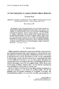
C(0) = IN’1 + 1 ND(G). BE0 The complexity is depending on both attributes and control nodes (the ones involved in the control structure of a member) and the predicates dominating them. As in the definition of the complexity of a program, we sum the total nesting depth of each method, and add the number of nodes of the object (both data and control nodes). When we define the Red(z) set of an attribute x, we involve the nodes from all the member graphs which predicate .z. The number of control nodes in the object graph is the sum of the number of control nodes of the member graphs. At the same time, each attribute node is counted only once. The definition reflects the common experience that good object-oriented programs have very strong bindings between the attributes and the methods inside the class and have very weak connections between different classes. The complexity of an individual member function does not depend on whether it works on global data or in a class attribute. However, the whole program can decrease its complexity if it uses member functions for accessing local data hidden in a class. See Figure 6 as an example. Here, we show a (simplified) date class. The class is represented by three
824
et-next-day I
Figure
6.
data members: day, month, and year denoted by dl, dz, and ds on Figure 6. We implemented two methods on the class: set-ne&month and set-next-day. We coded the predicate nodes as p1 ::= month == 12 p2 ::= p3 ::= p4 ::=
month == I or month == 3 or . ..or day == 31 day == 30
month == 12
and the other nodes as a 1s month := 1 b c e f
:= := := :=
g
:=
year := year+1 month := month+1 day := 1 set-next-month day := day+1
(For the sake of simplicity we ignored February and the leap-year problem.) the class can be computed based on Definition 20. Scope(pl) = {d2,d2,a,b9d3,d3,c) Scope(a) = (d2) Scope(b) = (d3 ,d3} Scope(c) = {d2,d2) Scope(p2) = {d2,p3,di,di,e,f,Pqlg} Scope(p3) = {di,dl,e,f,g) ScopeCpq) = {dl ,di ,e,f,g) Scope(e) = {dl} Scope(f) = 0 Scope(g) = {di,di) Pred(pi) = 0 PredCa) = {PI} PredCb) = {PI} PredCc) = {PI} Pred(p2) = 0 Pred(p3) = (P2) Pred(pq) = (P2) Pred(e) = {p2,p3,p4)
The complexity of
The Structured Complexity Pred(f)
= {I’2 ,I’3 ,l’4) P-d(g) = (~2 ,p3 ,~4) Pred(dl)=(p2,p2,p3,p3,P4,P4,e,g,g) Pred(d2)={pi,pl,p2,a,c,c) Pred(dg)={pl ,pi ,b,b) Thus, IN’1 = 13, ND(G) = 33, and C(O) = 46. REMARK 1. In a real object-oriented language when we implement a class, member functions often call another member function (from the same or from a different class). In Figure 6, member function set-next-day calls setnext_month, another member function of the same class. AS we have seen in the procedural programs, we can represent the called procedure in the caller as an elementary node. The called procedure should be represented as a member graph in the same or in a different object. As with the complexity of the program, such constructions regularly decrease the complexity of the caller function and the class. REMARK 2. It is possible that a class has only data and has no member function. This is a kind of grouping data. However, this is not a supported technique; it is syntactically correct to write in C-t-i-: class
date
//
public : int year,
example
month,
4. I.
day;
1; In our model, we can still compute the complexity of this class, which is the number of the attributes. This is in harmony with common sense. Similarly, if a class has no attributes at all, its complexity is the sum of the individual members. This “class” is an ordinary function libmry. REMARK 3. The model we introduced does not make a distinction between public and private data and method. The access right of a member does not influence the complexity of the class itself. Let us see the two C++ class definitions below. class
date
//
example
4.2.
public : void setnext_monthO { if ( month == 12 ) { month = I; else { month = month + I; } int
year,
month,
year = year + I;
}
day ;
1; class
date
//
example 4.3.
public: void set-next-month0 { if ( month == 12 > ( month = 1; year = year + 1; } else { month = month + 1; } private : int year,
month,
day;
Can an ordinary C++ programmer see the differences in complexity between the two definitions? We can hardly say yes. However, there could be differences in the complexity of the client code,
826
A.
F~)THI
et al
which uses the class. If the client accesses the attributes of function, we can replace its subgraph in the client code in the complexity of the client code. If the client accesses the this. Using Example 4.2, the client programmer can choose Example 4.3, he is forced to choose the better one.
the class via the setnextrmonth the known way. This decreases attributes directly, we cannot do whichever way; with the code in
It is easy to see that our measure fulfills all the axioms proposed in 1111. However, it was shown by Cherniavsky and Smith [12] that Weyuker’s properties do not guarantee the correctness of a measure. We still believe that those axioms are minimal requirements, and a good measure should comply with them.
5. CLASS
RELATIONSHIPS
A data member of a class is marked with a single data node regardless of its internal complexity. If it represents a complex data type, its definition should be included in the program and its complexity is counted there. Up to the point where we handle this data as an atomic entity, its effect to the complexity of the handler code does not differ from the effect of the most simple (built-in) types. In a C++ program a correctly written date class implements the assign (=), the less-than (x
=
y;
Here, we use the member functions of date, the calls of which have constant complexity regardless of its implementation. However, if we break the encapsulation of class date (i.e., we directly access its components), the data reference edges connect the handler code to the internal representation and increment its complexity. Once again, we stress this fact has to do with the private or public members only in an indirect way: as far as we use the methods to handle data, it does not matter whether the components are public or private. Of course, the compiler supports this strategy only when we made our components private. Inheritance is handled in a similar way. Code of the derived class in most cases (but not necessary) refers to the methods and/or data members of the base class(es). These references (method calls or data accesses) are described in the very same way as we did in the case of procedural programs. The motivation here is again to derive complexity from the basic, paradigmindependent program elements. class
diary
{ public : string
: public
date
event;
1; Here, we used inheritance to extend the interface of date. There is no communication between the basic class and the new attribute(s) and methods (not shown here). In this case, the increase of complexity is the complexity of the new attributes and methods of the derived class. In the case where derived class has a stronger binding to the base class(es), we use the known notations. Base class attributes accessed by derived methods are expressed by data reference edges; base class methods called by derived methods are represented by their nodes in the control graph of the caller method. It is easy to see that the less the data reference edge crosses the border of the classes, the lower the complexity number we achieve. We stress again; this is rather a result of the specially organized code and not the basis of our definition.
The
Structured
Complexity
827
6. CONCLUSIONS The complexity measure studied here expresses the structural complexity of the program. We investigated the complexity measures given in [6-g], and found them suffering from a common problem-that they, while computing the complexity of a given program, did not take the role of either the modularization or the data used into account. On the basis of the previous efforts of Howatt and Baker [9], we suggested a new measure of program complexity, which reflects our psychological feeling that the main concepts of object-oriented programming methodology help us to decrease the total complexity of a program. The notion of inheritance allows us actually to hide a class internal representation, further decreasing the sum of complexity, of course adding to the complexity of the inheritance hierarchy. Our measure is based on paradigm-independent notions. This makes it possible to use this method in a mixed-paradigm environment-a growing claim in modern programming languages today. Well-designed, fully implemented class interfaces, strong bindings inside a class, and weak bindings between a class and its environment, as well as good inheritance hierarchy are still major components to decrease complexity, yet they are not the base points to define our measure but a result of a specially organized code. There is a gnu g++ software tool under development implementing our new measure. We can apply this tool to C and C++ sources to gain a number of quantitative results with our measure.
REFERENCES 1. S. Henry and D. Kafura, Software structure metrics based on information flow, IEEE tins. So&are En& neering 7, 510-518, (1981). 2. B. Stroustrup, The C++ Programming Language, Addison-Wesley, (1997). 3. G. Kiczales, Aspect-oriented programming (AOP), ACM Computing Surueys 28 (4es). (1996). 4. J.O. Coplien, Multi-Paradigm Design for C++, Addison-Wesley, (1998). 5. K. Czarnecki and U.W. Eisenecker, Generative Programming, Addison-Wesley, (2000). 6. P. Piwowarski, A nesting level complexity measure, ACM Sigplan Notices 17 (Q), 44-50, (1982). 7. W.A. Harrison and K.I. Magel, A complexity measure based on nesting level, ACM Sigplan Notices 16 (3), 63-74, (1981). 8. W.A. Harrison and K.I. Magel, A topological analysis of the complexity of computer programs with less than three binary branches, ACM Sigplan Notices 16 (4), 51-63, (1981). 9. J.W. Howatt and A.L. Baker, Rigorous definition and analysis of program complexity measures. An example using nesting, The Journal of Systems and Software 10, 139-150, (1989). 10. Dunsmore and Gannon. 11. E.J. Weyuker, Evaluating software complexity measures, IEEE pans. Software Engineering 14, 1357-1365, (1988). 12. J.C. Cherniavsky and C.H. Smith, On Weyuker’s axioms for software complexity measures, IEEE Tbns. Software Engineering 17, 1357-1365, (1991). 13. E.W. Dijkstra, A Discipline of Programming, Prentice-Hall, Englewood Cliffs, NJ, (1976) 14. A. F6thi and J. Nyeky-Gaizler, A theoretical approach of objects and types, In Proceedings of the Second Symposium on Programming Languages and Software Tools, Pirkkala, Finland, August 21-23, 1991, (Edited by K. Koskimies and K.-J. Raiha), Report A-1991-5, (August 1991). 15. T.J. McCabe, A complexity measure, IEEE Trans. Software Engineering 2 (4), 308-320, (1976). 16. B. Meyer, Object-Oriented Software Construction, Prentice-Hall, New York, (1988). 17. L. Varga, A new approach to defining software design complexity, In Shijting Paradigms in Software Engineering, (Edited by R. Mittermeier), pp. 198-204, Springer-Verlag, Wien, (1992), 18. J.S. Davis and R.J. LeBlanc, A study of the applicability of complexity measures, IEEE ‘Pmns. So&are Engineenng 14, 1366-1372, (1988). 19. K.B. Lakshmanan, S. Jayaprakash and P.K. Sinha, Properties of control-flow complexity measures, IEEE 7hns. Software Engineering 17, 1289-1295, (1991). 20. J. Tian and M.V. Zelkowitz, Complexity measure evaluation and selection, IEEE hns. Sojtvjare Engineering 21, 641-650, (1995).