Symbolic dynamics and characterization of complexity - Science Direct

Physica D 51 (1991) 161-176 North-Holland

Symbolic dynamics and characterization of complexity Bai-lin H a o 1 Institute for Physical Science and Technology and Department of Physics, University of Maryland, College Park, MD 20742, USA

Symbolic dynamics deals with robust properties of dynamics without digging into numbers. For one-dimensional maps there have been some new results (periodic window theorem, generalized composition rule, construction of median words without using harmonics and antiharmonics, incorporation of discrete symmetry to analyze symmetry breaking and symmetry restoration, etc.) This new understanding has been applied to ordinary differential equations, in particular, the systematics of stable periodic solutions in the Lorenz model has been shown to be given basically by symbolic dynamics of the cubic map. Symbolic dynamics may be used to extract invariant characteristics from time series. Its relation with grammatical complexity will also be commented on.

I. Introduction

Symbolic dynamics provides a rigorous way of looking at "real" dynamics with finite precision. It is a way of coarse-graining or reduction of description. The basic idea is quite simple. One divides the phase space into a finite number of partitions and labels each partition with a symbol (a letter from some alphabet). Instead of representing the trajectories by infinite sequences of n u m b e r s - i t e r a t e s from a discrete map or sampled points along the trajectories of a continuous flow - , one watches the alternation of symbols. In so doing, one loses a great amount of detailed information, but some of the invariant, robust properties of the dynamics may be kept, e.g. periodicity, symmetry, or chaotic nature of an orbit. According to a historical note in ref. [1], the use of symbols dated back to 1857. It was Morse who first recognized the role of symbolic description for dynamics [2]. His 1938 paper with Hedlund [3] was simply entitled "Symbolic Dynamics". Bowen, Ruelle, and Sinai used symbolic dynamics in ergodic theory, see, e.g., the review IOn leave from the Institute of Theoretical Physics, Academia Sinica, Beijing, China.

by Alekseev and Yakobson [4], which, in fact, was an appendix to a collection of Russian translations of Bowen's papers [5]. The applied aspects of symbolic dynamics, which is the main subject of the present survey, has developed since the paper of Metropolis, Stein and Stein [6] (hereafter abbreviated as MSS), produced at the Los Alamos National Laboratory. The kneading theory of Milnor and Thurston [7], the lecture of Guckenheimer [8], and, especially, the paper by Derrida, Gervois and Pomeau [9] (hereafter abbreviated as DGP), contained further results on symbolic dynamics of maps of the interval. The monograph of Collet and Eckmann [10], though written in a fairly mathematical style, summarized what had been known by the end of 1970's. Through the 1980's there has been steady progress in understanding symbolic dynamics of maps with multiple critical points, with discontinuities, and in applying the knowledge to ordinary differential equations and time series. Most of these results are still scattered in the literature; we will try to summarize some of them. The layout of this paper is as follows. In section 2 we first give a very concise yet selfcontained summary of symbolic dynamics of one-dimensional mappings, then discuss a few

0167-2789/91/$03.50 © 1991- Elsevier Science Publishers B.V. (North-Holland)

B.-L. Hao /Symbolic dynamics and complexity

162

recent results related mostly to maps with multiple critical points or discontinuities. A symbolic dynamics analysis of symmetry breakings and restorations will serve as a bridge to the Lorenz model. Section 3 contains a few technical improvements in calculating topological entropy from symbolic sequences and some remarks on characterizing the complexity of symbolic sequences by using the notion of grammatical complexity. In section 4 we will discuss the application of symbolic dynamics to numerical study of ordinary differential equations, both autonomous and periodically driven ones, as well as symbolic dynamics from time series. The last section is devoted to a brief discussion of future developments.

2. Symbolic dynamics of one-dimensional maps Owing to the nice ordering property of the real line, symbolic dynamics of one-dimensional maps may be worked out in great detail. Since a substantial exposition of this subject has a p p e a r e d in a recent m o n o g r a p h [11] and in a comprehensive review [12], we will confine ourselves to a concise summary that threads the main results together.

gets a numerical sequence

Xo,

= f ( x 0 ) , x2 = f ( x l ) . . . . .

x,_~= f(xn_2),x,,=f(x~_l),....

(2)

We juxtapose (2) with a symbolic sequence and call it by the number x0 which has originated the numerical sequence: x0 = ~0~rl~r2... ~,_ vrn . . . .

(3)

where ~r~ stands for one of the symbols Si or Ci, depending on whether x i belongs to the corresponding subinterval or coincides with a turning point. If we want to reverse the sequence (2), expressing x0 through x , , we must be more careful in writing down (2) by indicating which of the monotone branches of f has been used at each iteration. To do so, we attach a subscript ~r to f. Clearly, the symbol ~ is chosen by the argument of f:

Xo, x, =L,,( xo), x2 = L , ( x , ) . . . . . x , =f~,, , ( x , _ , ) . . . . .

(4)

Now we are in a position to reverse (4) and get, e.g.,

2.1. The number-symbol-inverse function correspondence

x 0 = f ; ~ ,, o f ; , o . . . o f ; , -1 ,(Xn).

Consider a nonlinear function f(/z, x), which maps points from an interval I into the same interval:

TO simplify the notation, we will denote each inverse monotone branch f ~ l by its subscript, i.e. we define

Xn+l=f(tz,Xn),

~r(y) =-f¢'(y),

Xn~I,

(1)

w h e r e / x stands for one or more parameters. The function f may have several m o n o t o n e branches, divided by turning points, denoted symbolically by Ci (called also critical points). For smooth maps the derivative d f / d x vanishes at x = C~. The turning points C i and the end points of the interval I divide I into subintervals I i. We label each of I i by a symbol S i. By iterating (1), one

(5)

(6)

where o- is one of the symbols S i. For example, the logistic map

x n + , = t x - x 2, x , ~ ( - 1 , 1 ) ,

/x~(0,2)

(7)

has two inverse branches:

R(y)=~/I.t-y,

L(y)= -gr~-y.

(8)

B.-L. Hao /Symbolic dynamicsand complexity

parametrize a map by its independently changing kneading sequences.

Now eq. (5) reads x0=~0O~lO...O%_l(Xn).

163

(9)

2.3. The word-lifting technique Eqs. (2), (3), and (9) give the n u m b e r - s y m b o l inverse function correspondence.

2.2. The kneading sequence In the unimodal map (7) the iterate of the critical point C = 0 leads to the rightmost point f ( C ) on the interval that one can ever reach by iterating the map from any point on the interval. The point f ( C ) thus starts a special symbolic sequence, called the kneading sequence by Milnor and Thurston [7]. According to our convention (3) the kneading sequence is named f ( C ) and sometimes we denote it by K (for kneading). For instance, at the parameter value/z = 1.85 the map (7) has a kneading sequence

K =f(C) = RLLRLRLRRL ....

Among all possible kneading sequences there are two important and well-understood types, namely, superstable periodic sequences K = (,~CY ° that contain the critical point C (we consider unimodal maps for the time being), and eventually periodic sequences K = p)t~, where ~, p, and A are strings made of R and L. It often happens that, given a concrete map, one wishes to look at a particular case when the map has a given kneading sequence. How could one determine the parameter value? It turns out that for the two above-mentioned types of kneading sequences the answer follows from the number-symbol-inverse function correspondence. A kneading sequence of type (,~C) ® means we have

(10) f(c)

The second iterate of C, i.e. f2(C), gives the leftmost point that one can ever reach by iterating the map twice starting from any point on the interval. All the interesting dynamics takes place on the subinterval [f2(C),f(C)] of I. Once a point is in this subinterval, its iterates can never get out. Therefore, this subinterval defines an invariant dynamical range. In principle, one can choose an initial point outside this subinterval, but after a trivial transient (in fact, a few iterations), it will fall into the invariant dynamical range. For maps with multiple critical points each C i leads to a kneading sequence; one collects the dynamical range of all turning points and finds the overall range of interest dynamics. In what follows we will concentrate on invariant dynamical range only, neglecting trivial transients. With our convention (3) each kneading sequence is represented by a number. This number may be taken as the parameter for the map. This happens to be very convenient for maps with multiple critical points. In other words, one can

= Zczc

....

Using (9) we get an equation

f ( C ) =~Y(C),

(11)

where ,~(y) should be understood as a composite function made of R and L. For an eventually periodic sequence p)t®, similar consideration leads to a pair of equations

f ( c ) =p(v),

v

(12)

where p and A should again be understood as composite functions. For unimodal maps the four-piece chaotic bands merge into two bands when the kneading sequence is K = RLRR(RL) ®. Eq. (12) then reads

f(C)=RoLoRoR(v),

v=RoL(v).

For the logistic map (7) f ( C ) =/z, R ( y ) and L ( y ) are given by (8), one has to solve the following

164

B.-L. Hao /Symbolic dynamics and complexity

pair of iterated equations:

that differ from each other:

Xl=X*o- ....

with any reasonable initial conditions, say, /x 0 = 2.0, u 0 = 1.95, one gets p. = 1.4303576... and u = 1.3248379 . . . . For maps with more than one kneading sequence the word-lifting technique no longer gives numbers, but leads to equations of curves or surfaces in the parameter space. The loci of superstable kneading sequences in the parameter space have been called skeletons [13]. Skeletons have been calculated for the sine-square map [14], the circle map [13, 15, 16], the general cubic map [17-20], the gap map [21] and the "Lorenz type" map [22] (see section 2.12).

2. 4. Ordering of symbolic sequences The ordering of symbolic sequences is based on the natural order of real numbers on the interval, e.g.

L 3,

2-->3,

3-->1+2,

I

leading to the Stefan matrix 0 T= 0 1

0 0 1

1 1 0

I i

(50)

I

I

I

The largest eigenvalue /~max= ~ - of T determines the topological entropy h = 71 log 2. 3.3. Grammatical complexity

It has been pointed out by several authors, see, e.g., ref. [46], that topological entropy is rather a measure of randomness, not complexity. Complexity should have a closer relation with the number of grammatical rules which allow or forbid strings of letters to appear in symbolic sequences, viewed as a certain language made of letters from a finite alphabet. This provides us with a suitable setting to invoke the theory of grammatical complexity as Wolfram [47] first did for cellular automata. Not going into various definitions of complexity, see, e.g. [48-53], we continue with our simple example of Stefan matrix to show the connection. If we take the intervals 1, 2, and 3 in fig. 3 as nodes (states) of a graph, then the Stefan matrix gives the transition function [45] for the finite automaton, which accepts all admissible sequences under K = R L R ~. In fact, this is the type of automaton, used in, e.g. ref. [52]. All kneading sequences of (,~C) ~ and pA~ types can only lead to finite automata, lying at the lowest level of the grammatical complexity ladder (so-called Chomsky hierarchy [45]). In particular, all OA= maps have finite entropy, but zero complexity [52]. In order to look for finite complexity sequences, one has to study limits of either ( Z C ) ~ or OA= type sequences. An example of the first type is the limit of the Fibonacci sequence (23) or the Feigenbaum period-doubling sequence (17).

F.4

F...

~:-- I

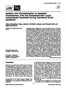
Fig. 4. The structure of Stefan matrix for the period F. word in the Fibonacci sequence. Solid line indicates where the matrix elements are 1; all other elements are zero.

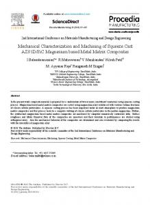
The second type may be represented by the limit of the 2" ~ 2 n - I band-merging points (see section 2.9). The structure of the limiting automata can be seen from the corresponding Stefan matrices. The Stefan matrix for the period F, (the nth Fibonacci number) member in (23) has the structure shown in fig. 4. It consists of four nonzero blocks with the size of the blocks growing with period. The Stefan matrix for the band-merging limit shows a little more structure: there is a growing number of blocks, but the general pattern remains regular. The case of 64 ~ 32 band-merging point is shown in fig. 5. For the 2 n ~ 2 n - 1 merging point the structure of the Stefan matrix is given by the

Fig. 5. The structure of Stefan matrix for the 2 n----~2 n - I band-merging point (shown the n = 6 case).

B.-L. Hao /Symbolic dynamics and complexity

174

following equality: 2 n-1 + 1 + 2 n-2 + 3 ( 2 n - 3 + 2~-4 + ... + 2 + 1 ) + 2 = 3 × 2 ~ 1. Some definitions [48, 52] of complexity give an infinite value at the Feigenbaum accumulation point, whereas we know the attractor is only quasiperiodic and symbolic dynamics is quite simple (R *n, n ~ o0). In a sense, both entropy calculation and grammatical approach start from the same Stefan matrix; different numerical characteristics come essentially from different definitions of the interested quantities. Anyway, the Stefan matrix, which is fairly easy to derive from the symbolic sequences, may serve as a convenient tool.

4. Application to ODE's and time series

In dissipative systems with only one positive Lyapunov exponent, i.e. one locally stretching direction, phase volume contraction may result in one-dimension like objects in certain sections. Although complicated foldings may give rise to a Cantor set structure in other directions, there is good hope to compare the dynamics with that of one-dimensional maps, especially when one confines oneself to periodic solutions of short periods. The systematics of periodic solutions alone, if found, may tell something about the nature of the chaotic regime even without going through the hard work of characterizing the chaotic attractors. For the time being, this is still a sort of experimental mathematics, based on numerical evidence. Indeed, we have accumulated some experience on ordinary differential equations, both autonomous and periodically forced systems.

4.1. Periodically driven planar systems In periodically driven systems the period of the external force serves as a natural unit to measure

all other periods in the dynamics and stroboscopic sampling at multiples of the forcing period allows for very high frequency resolution. If the external force is given as an infinite train of 6-functions (the Dirac comb) and the unforced system has analytical solutions, then the system may be transformed exactly into two-dimensional maps which may save computing time considerably. One may assign letters to the numerically observed orbits and then compare them with the systematics of periods in known maps. Perhaps the most detailed studied system is so-called forced Brusselator (for a recent review see section 5.7 in ref. [11]). O t h e r examples include a few limit cycle oscillators [54, 55], the forced van der Pol equation [56], etc. In all these cases the systematics of periodic solutions were given by symbolic dynamics of two letters, either that of the MSS sequence or that of the Farey sequences. The transition between these two types of symbolic sequences has not been understood fully yet (see, however, a recent p a p e r [57]).

4.2. The Lorenz model The celebrated Lorenz model [58] is an autonomous system of three ordinary differential equations. It is invariant under the discrete transformations x ~ - x , y~-y, which make it closer to the antisymmetric cubic m a p (25) rather than the H f n o n map. This cubic nature may be seen clearly in the (Xi+l,Xi) o r (Yi+l, Yi ) first return maps, recalculated from the Poincar6 maps (xi, Yi). We have assigned three letters to the numerically observed periodic orbits and 47 out from 53 primitive periods along the most studied direction in the p a r a m e t e r space ( g = 10, b = ~8, r varies from 25 to 350) fit into the order of the cubic map [59]. A by-product of this painstaking work is now we have an absolute nomenclature of periods for the Lorenz system, which coincides with the results of a frequency calibration curve, obtained earlier by extensive power spectrum analysis of the Lorenz equations [60].

B.-L. Hao / Symbolic dynamics and complexity 4.3. Symbolic dynamics from time series In contradistinction from model study of maps and differential equations where one deals with families of dynamical systems, the study of time series usually involves single orbits and the job consists in characterization or comparison of orbits. To generate a symbolic sequence from a numerical time series requires an understanding of the dynamics, obtained by, say, reconstructing the phase portrait in some embedding space. Experimental data from the BelousovZhabotinsky reaction have been analyzed by using symbolic dynamics [61]. In principle, one can estimate topological entropy by simply counting the occurrence of symbolic strings of various lengths (this was applied to model series in ref. [62]), and a more detailed counting of the frequency of occurrence of these strings would give an estimate of metric entropy. A further task consists in deriving the grammatical rules from the symbolic sequences. T h e r e has been some progress on time series from models [48].

5. Discussion We hope that the foregoing review has shown that symbolic dynamics is no longer an abstract chapter of mathematics. It has become a practical tool to study dynamics. The empirical use of symbolic dynamics to differential equations and time series remains to be justified and its limitations to be clarified. We would like to list briefly a few topics awaiting further elaboration. The first challenge is how to extend symbolic dynamics to higher dimensional systems. The basic idea of coarse-graining works, of course, in any dimension, the problem being the lack of good generating partitions and natural ordering. There has been some progress with the H6non map [63, 64], and with the Lozi m a p [64, 65]. The application of symbolic dynamics to Hamiltonian systems is also a long-standing problem. As regards the experimental application of symbolic dynamics to differential equations, the

175

whole approach is still in its beginning stage. We have to accumulate more results on various systems and to automatize the time-consuming numerical work before, say, any general classification scheme based on symbolic dynamics may be worked out. The same may be said about time series. Grammatical complexity may provide a better way of comparing symbolic sequences, but even the very definition of grammatical complexity requires refinement. At least, one has to go beyond quasiperiodic attractors and to distinguish really chaotic attractors in their complexity. The Chomsky hierarchy may not be the most suitable scale for dynamics.

Acknowledgements The author thanks the Aspen Center for Physics and the Center for Nonlinear Studies at Los Alamos National Laboratory where the final manuscript of this p a p e r was written. We thank Drs. Auerbach, R. Badii and J.P. Crutchfield for sending their papers prior to publication. Collaboration with Dr. Weimou Zheng has significantly deepened my understanding of symbolic dynamics. Discussions with Drs. L.P. H u r d and Wentian Li on grammatical complexity was also very instructive for me.

References [1] I. Procaccia, S. Thomae and C. Tresser, Phys. Rev. A 35 (1987) 1884. [2] M. Morse, Trans. Am. Math. Soc. 22 (1921) 84. [3] M. Morse and G.A. Hedlund, Am. J. Math. 60 (1938) 815; reprinted in Collected Papers of M. Morse, Vol. 2 (World Scientific, Singapore, 1986). [4] V.M. Alekseev and M.V. Yakobson, Phys. Rep. 75 (1981) 287. [5] R. Bowen, Methods of Symbolic Dynamics, a collection of Bowen's papers in Russian translation, ed. V.M. Alekseev (Mir, Moscow, 1979). [6] N. Metropolis, M.L. Stein and P.R. Stein, J. Combinat. Theory A 15 (1973) 25.

176

B.-L. Hao /Symbolic dynamics and complexity

[7] J. Milnor and W. Thurston, preprint (1977); in: Lecture Notes in Mathematics, Vol. 1342 (Springer, Berlin, 1988) p. 465. [8] J. Guckenheimer, J. Moser and S.E. Newhouse, Dynamical Systems, C.I.M.E. Lectures, Progress in Mathematics 8 (Birkh/iuser, Basel, 1980). [9] B. Derrida, A. Gervois and Y. Pomeau, Ann. Inst. Henri Poincar~ 29A (1978) 305. [10] P. Collet and J.-P. Eckmann, Iterated Maps on the Interval as Dynamical Systems (Birkhiiuser, Boston, 1980). [11] B.-L. Hao, Elementary Symbolic Dynamics and Chaos in Dissipative Systems (World Scientific, Singapore, 1989). [12] W.-M. Zheng and B.-L. Hao, in: Experimental Study and Characterization of Chaos, Vol. 3 of Directions in Chaos, ed. Hao Bai-lin (World Scientific, Singapore, 1990). [13] J. B~lair and L. Glass, Physica D 16 (1985) 143. [14] H.-J. Zhang, J.-H. Dai, P.-Y. Wang, C.-D. Jin and B.-L. Hao, Chin. Phys. Lett. 2 (1985) 5; Commun. Theor. Phys. 8 (1987) 281. [15] R.S. MacKay and C. Tresser, Physica D 19 (1986) 206; 29 (1988) 427. [16] W.-Z. Zeng and L. Glass, Physica D 40 (1989) 218. [17] R.S. MacKay and C. Tresser, Physica D 27 (1987) 412; J. London Math. Soc. 37 (1988) 164. [18] R.S. MacKay and J.B.J. van Zeits, Nonlinearity 1 (1988) 253. [19] J. Ringland and M. Schell, Phys. Lett. A 136 (1989) 379. [20] J. Ringland and M. Schell, Universal geometry in the parameter plane of maps of the interval, preprint (1989); Genealogy and bifurcation skeleton for periodic orbits of the iterated two-extremum map of the interval, preprint (1989), submitted to SIAM J. Math. Anal. [21] W.-M. Zheng and L.-S. Lu, Chaos boundary of the gap map, preprint (1990). [22] W.-M. Zheng, Phys. Rev. A 42 (1990) 2076. [23] W.-Z. Zeng, M.-Z. Ding and J.-N. Li, Commun. Theor. Phys. 9 (1988) 141. [24] W.-M. Zheng, J. Phys. A 22 (1989) 3307. [25] W.-Z. Zeng, B.-L. Hao, G.-R. Wang and S.-G. Chen, Commun. Theor. Phys. 3 (1984) 283. [26] G.-R. Wang and S.-G. Chen, Acta Phys. Sinica 35 (1986) 58 [in Chinese]. [27] N.J. Fine, Illinois J. Math. 2 (1958) 285. [28] E.N. Gilbert and J. Riodan, Illinois J. Math. 5 (1961) 657. [29] W.-Z. Zeng, Commun. Theor. Phys. 8 (1987) 273. [30] W.-Z. Zeng, Chinese Phys. Lett. 2 (1985) 429. [31] B.-L. Hao and W.-Z. Zeng, in XV Int. Colloq. on Group Theoretical Methods in Physics, ed. R. Gilmore (World Scientific, Singapore, 1987) p. 199. [32] D. D'Humieres, M.R. Beasley, B.A. Huberman and A. Libchaber, Phys. Rev. A 26 (1982) 3483. [33] K. Kumar, A.K. Agarwal, J.K. Bhattacharjee and K. Banerjee, Phys. Rev. A 35 (1987) 2339. [34] J.W. Swift and K. Wiesenfeld, Phys. Rev. Lett. 52 (1984) 705. [35] K. Weisenfeld, E. Knobloch, K.F. Miracky and J. Clarke, Phys. Rev. A 29 (1984) 2102.

[36] W.-M. Zheng and B.-L. Hao, Int. J. Mod. Phys. B 3 (1989) 1183. [37] P. Chossat and M. Golubitsky, Physica D 32 (1988) 423. [38] K.G. Szabo and T. T~l, J. Stat. Phys. 54 (1989) 925. [39] M.C. de Sousa Vieira, E. Laso and C. Tsallis, Phys. Rev. A 35 (1987) 945. [40] W.-M. Zheng, Phys. Rev. A 39 (1989) 6608. [41] Lu Lisha, Symbolic dynamics of the one-dimensional gap map, Master Thesis, Institute of Theoretical Physics (Beijing, 1989), unpublished. [42] C.S. Hsu and M.C. Kim, Phys. Rev. A 31 (1985) 3253. [43] P. Collet, J.P. Crutchfield and J.-P. Eckmann, Commun. Math. Phys. 88 (1983) 257. [44] J.P. Crutchfield and N.H. Packard, Physica D 7 (1983) 201. [45] J.E. Hopcroft and J.D. Ullman, Introduction to Automata Theory, Languages, and Computation (AddisonWesley, Reading, MA, 1979). [46] P. Grassberger, Int. J. Theor. Phys. 25 (1986) 907. [47] S. Wolfram, Commun. Math. Phys. 96 (1984) 15. [48] P. Grassberger, Z. Naturfosch. 43a (1988) 671. [49] J.P. Crutchfield and K. Young, Phys. Rev. kett. 63 (1989) 105. [50] J.P. Crutchfield and K. Young, Computation at the onset of chaos, preprint. [51] G. D'Alessandro and A. Politi, Phys. Rev. Lett. 64 (1990) 1609. [52] D. Auerbach and I. Procaccia, Phys. Rev. A 41 (1990) 6602. [53] R. Badii, Quantitative characterization of complexity and predictability, preprint. [54] E.-J. Ding, Phys. Rev. A 34 (1986) 3547; 35 (1987) 2669; 36 (1987) 1488. [55] D.L. Gonzalez and O. Piro, Phys. Rev. Lett. 50 (1983) 870. [56] E.-J. Ding, Phys. Scripta 38 (1988) 9. [57] J. Ringland, N. Issa and M. Schell, Phys. Rev. A 41 (1990) 4223. [58] E.N. Lorenz, J. Atmosph. Sci. 20 (1963) 130. [59] M.-Z. Ding and B.-L. Hao, Commun. Theor. Phys. 9 (1988) 375. [60} M.-Z. Ding, B.-L. Hao and X. Hao, Chinese Phys. Lett. 2 (1985) 1. [61] R.H. Simoyi, A. Wolf and H.L. Swinney, Phys. Rev. Lett. 49 (1982) 245; K. Coffman, W.D. McCormick and H.L. Swinney, Phys. Rev. Lett. 56 (1986) 999. [62] C. Kahlert and O.E. R6ssler, Z. Naturforsch. 39a (1984) 1200. [63] P. Grassberger and H. Kantz, Phys. Lett. A 113 (1985) 235. [64] P. Cvitanovic, G.H. Gunaratne and I. Procaccia, Phys. Rev. A 38 (1988) 1503. [65] W.-M. Zheng, Symbolic dynamics of the Lozi map, in: Chaos, Solitons and Fractals (1991), in press.