The Subspace Model: Shape-based Compilation ... - Semantic Scholar

The Subspace Model: Shape-based Compilation for Parallel Systems by

Kathleen B. Knobe

B.S., Colorado State University (1972) M.A., Boston University (1980) Submitted to the Department of Electrical Engineering and Computer Science in partial ful llment of the requirements for the degree of Doctor of Philosophy at the MASSACHUSETTS INSTITUTE OF TECHNOLOGY January 1997

c Massachusetts Institute of Technology 1997 The author hereby grants to MIT permission to reproduce and to distribute copies of this thesis document in whole or in part. Signature of Author Department of Electrical Engineering and Computer Science January 10, 1996 :::::::::::::::::::::::::::::::::::::::::::::::

Certi ed by

::::::::::::::::::::::::::::::::::::::::::::::::::::::::

Accepted by

William J. Dally Arti cial Intelligence Laboratory Thesis Supervisor

:::::::::::::::::::::::::::::::::::::::::::::::::::::::

Arthur C. Smith Chairman, Departmental Committee on Graduate Students

2

The Subspace Model: Shape-based Compilation for Parallel Systems

by Kathleen B. Knobe Submitted to the Department of Electrical Engineering and Computer Science on January 10, 1997 in partial ful llment of the requirements for the Degree of Doctor of Philosophy in Computer Science.

Abstract

Subspace analysis is a target independent parallel compilation technique. It applies to a wide range of parallel architectures including vector, SIMD, distributed memory MIMD, shared memory MIMD, symmetric multiprocessors and VLIW systems. The focus of the subspace analysis is shape. The shape of an object is a subset of the iteration indices. Each index represents an axis of the object. The concept of shape is a hidden but crucial theme underlying the work in parallelism detection algorithms, many architecture speci c optimizations and many strategies for compiling to parallel programs. Parallelization is shape-based. So are a variety of optimizations (e.g., privatization), strategies (e.g., the replication of scalars in SPMD systems) and language issues (e.g., conformance in Fortran 90). Shape is of critical importance in parallel systems since a shape that is too small (has too few axes) can result in unnecessary serialization whereas a shape that is too large (has too many axes) can result in unnecessary computation and communication. Our goal is to unify and generalize existing shape-based analyses and strategies by attacking shape directly, instead of incorporating shape in dierent ways into a variety of distinct analyses. We present an algorithm that determines the natural shape of data objects and operations. There are two bene ts to this approach: The compiler for a given target is simpler, and a more signi cant portion of the compiler is independent of the parallel target architecture. If the input is explicitly parallel, subspace analysis performs shape-based optimizations, possibly increasing parallelism in the process. If the input is scalar, subspace analysis also acts as the parallelization phase. Thesis Supervisor: William J. Dally Title: Professor of Electrical Engineering and Computer Science

3

4

Acknowledgments

I owe thanks to many in this endeavor. 

My advisor, Bill Dally Your encouragement has been critical. Your advise on technical issues and career issues has been invaluable. But your most important contribution was the constant refrain: \Is that really necessary?" I've enjoyed working with you. Thank you Bill.



My friends from Compass To those who encouraged me to \go for it" when I was starting to think about returning to school, thanks for the great advice. To Joan Lukas for constant support and encouragement. Thank you for being there at every turn, major and minor. To Pat Timpanaro for listening. You never seem to tire of my stories of stress. Thanks. To Je Ives for providing me with parking in Cambridge. Those who have ever tried to park in Cambridge know what a valuable contribution that is! You saved me many long walks in hot, humid summers and the icy, windy winters. I imagine you also saved me from several bouts of the u.



My fellow grad students To the gang on the sixth oor, especially Fred Chong, Don Yeung, John Kubiatowicz, Ellen Spertus and Rich Lethin, for all the standard fellow grad student stu: commiseration, advise, constructive criticism, support, junk food and humor. To David Shoemaker for enlivening the lunch time political discussions by consistently providing the minority opinion. Lunch will never be the same. A second thanks to Fred Chong. Without your timely advise about the MIT bureaucracy and the job search, I'd still be in NE43. 5



My friends outside the computing community I seem to have taken a long but unintentional leave of absence. I'm happy to be back. I hope you still remember me.



To Digital's Cambridge Research Lab Thanks for giving me both a great reason to nish and the time to do so.



My family Thanks to my son, Joshua. Its been great fun cheering each other on. Congratulations on getting to the nish line rst. Must be because I'm the better cheerleader (smile). Thanks to my husband, Bruce, not only for the usual support and encouragement, which you provided in abundance, but for helping me get to the point where I could consider embarking on this endeavor in the rst place.

6

Contents 1 Overview

1.1 The Problem: The Current State-of-the-Art : : : : : : 1.2 The Solution: The Subspace Model : : : : : : : : : : : 1.2.1 Natural Subspaces : : : : : : : : : : : : : : : : 1.2.2 Operational Subspaces : : : : : : : : : : : : : : 1.2.3 Expansions : : : : : : : : : : : : : : : : : : : : 1.3 Subspace Analysis in the Context of Full Compilation : 1.4 Contributions : : : : : : : : : : : : : : : : : : : : : : : 1.5 Organization : : : : : : : : : : : : : : : : : : : : : : :

2 Natural Subspaces

2.1 Input : : : : : : : : : : : : : : : : : : : : : : : : 2.2 Core Natural Subspace Algorithm : : : : : : : : 2.2.1 Core Language Restrictions : : : : : : : 2.2.2 Core Concepts and Terminology : : : : : 2.2.3 Core Algorithm: High level Description : 2.2.4 Core Algorithm : : : : : : : : : : : : : : 2.2.5 Core Algorithm: Analysis : : : : : : : : 2.3 Relaxing the Language Restrictions : : : : : : : 2.3.1 Array Subscripts : : : : : : : : : : : : : 2.3.2 I/O : : : : : : : : : : : : : : : : : : : : : 2.3.3 Explicit parallelism : : : : : : : : : : : : 2.3.4 Intrinsics : : : : : : : : : : : : : : : : : : 7

: : : : : : : : : : : :

: : : : : : : : : : : :

: : : : : : : : : : : :

: : : : : : : : : : : :

: : : : : : : : : : : : : : : : : : : :

: : : : : : : : : : : : : : : : : : : :

: : : : : : : : : : : : : : : : : : : :

: : : : : : : : : : : : : : : : : : : :

: : : : : : : : : : : : : : : : : : : :

: : : : : : : : : : : : : : : : : : : :

: : : : : : : : : : : : : : : : : : : :

: : : : : : : : : : : : : : : : : : : :

15 17 21 21 23 23 27 31 33

37 38 39 39 40 44 50 51 55 55 61 62 62

2.3.5 Alternate looping constructs : : : 2.3.6 Conditional Execution : : : : : : 2.3.7 Calling with Accurate Arguments 2.3.8 Returning Modi ed Arguments : 2.4 Summary : : : : : : : : : : : : : : : : :

3 Natural Expansions

3.1 Concepts and Terminology : : : : : 3.1.1 Cyclic Expansions : : : : : : 3.1.2 LHS and RHS References : 3.1.3 Loop Nests : : : : : : : : : 3.2 The Algorithm : : : : : : : : : : : 3.3 Relaxing the Language Restrictions 3.3.1 Predicates : : : : : : : : : : 3.3.2 I/O : : : : : : : : : : : : : : 3.4 Phase Integration : : : : : : : : : : 3.5 Summary : : : : : : : : : : : : : :

4 Intermediates

: : : : : : : : : :

: : : : : : : : : :

: : : : : : : : : :

: : : : : : : : : : : : : : :

: : : : : : : : : : : : : : :

: : : : : : : : : : : : : : :

: : : : : : : : : : : : : : :

: : : : : : : : : : : : : : :

: : : : : : : : : : : : : : :

Natural Subspace of Intermediates : : : : : : : : : : Operational Subspace of Intermediates : : : : : : : Implicitly Distributed Objects : : : : : : : : : : : : Expansions of Intermediates : : : : : : : : : : : : : Incorporating Predicates : : : : : : : : : : : : : : : Fragmentation : : : : : : : : : : : : : : : : : : : : : 4.6.1 Inconsistent Subspaces : : : : : : : : : : : : 4.6.2 Inconsistent Expansions : : : : : : : : : : : 4.6.3 A Distinction Between these Inconsistencies 4.7 Algorithm for Processing Intermediates : : : : : : : 4.8 Summary : : : : : : : : : : : : : : : : : : : : : : :

4.1 4.2 4.3 4.4 4.5 4.6

8

: : : : : : : : : : : : : : : : : : : : : : : : : :

: : : : : : : : : : : : : : : : : : : : : : : : : :

: : : : : : : : : : : : : : : : : : : : : : : : : :

: : : : : : : : : : : : : : : : : : : : : : : : : :

: : : : : : : : : : : : : : : : : : : : : : : : : :

: : : : : : : : : : : : : : : : : : : : : : : : : :

: : : : : : : : : : : : : : : : : : : : : : : : : :

: : : : : : : : : : : : : : : : : : : : : : : : : :

: : : : : : : : : : : : : : : : : : : : : : : : : :

: : : : : : : : : : : : : : : : : : : : : : : : : :

64 66 72 73 73

75 76 78 81 83 84 85 86 86 87 88

89

90 91 93 95 96 98 98 99 100 101 101

5 Restructure

5.1 Subspace Information : : : : 5.2 Subspace Normal Form : : : 5.3 Restructuring : : : : : : : : 5.3.1 The Algorithm : : : 5.3.2 An Example : : : : : 5.3.3 Ordering Fragments 5.4 Summary : : : : : : : : : :

: : : : : : :

: : : : : : :

: : : : : : :

: : : : : : :

: : : : : : :

: : : : : : :

: : : : : : :

: : : : : : :

: : : : : : :

: : : : : : :

: : : : : : :

: : : : : : :

: : : : : : :

6 Optimization

6.1 Redundant Expansion Elimination : : : : : : : : : 6.2 Generalized Common Subexpression Elimination : : 6.3 Optimization via Expression Reordering : : : : : : 6.3.1 Minimizing Subspaces : : : : : : : : : : : : 6.3.2 Minimizing Expansions : : : : : : : : : : : : 6.3.3 Maximizing the Potential for REE : : : : : 6.3.4 Maximizing the Potential for GCSE : : : : : 6.3.5 Integration of the Reordering Optimizations 6.3.6 Maximizing the Reordering Potential : : : : 6.4 Predicates : : : : : : : : : : : : : : : : : : : : : : : 6.5 Summary : : : : : : : : : : : : : : : : : : : : : : :

7 Experiments

7.1 Loop-based Parallelism : : : : : : : : : : : : : : : 7.2 Non-loop Concurrency : : : : : : : : : : : : : : : 7.2.1 Single Serial Expansion : : : : : : : : : : : 7.2.2 Concurrent Serial and Parallel Expansions 7.2.3 Two Concurrent Serial Expansions : : : : 7.3 Subspace Optimizations : : : : : : : : : : : : : :

8 Contributions

: : : : : :

: : : : : : : : : : : : : : : : : : : : : : : :

: : : : : : : : : : : : : : : : : : : : : : : :

: : : : : : : : : : : : : : : : : : : : : : : :

: : : : : : : : : : : : : : : : : : : : : : : :

: : : : : : : : : : : : : : : : : : : : : : : :

: : : : : : : : : : : : : : : : : : : : : : : :

: : : : : : : : : : : : : : : : : : : : : : : :

: : : : : : : : : : : : : : : : : : : : : : : :

: : : : : : : : : : : : : : : : : : : : : : : :

: : : : : : : : : : : : : : : : : : : : : : : :

103 103 105 106 107 108 111 115

117 119 120 121 122 123 123 124 125 130 131 134

135 135 139 141 142 142 144

147 9

8.1 Primary Claim : : : : : : : : : : : : : : : : : : : : 8.1.1 Data-Centric and Operation-Centric Models 8.1.2 Invariant Code Motion : : : : : : : : : : : : 8.1.3 Privatization : : : : : : : : : : : : : : : : : 8.1.4 Owner-Computes : : : : : : : : : : : : : : : 8.1.5 Replication of Scalars : : : : : : : : : : : : : 8.1.6 Conformance : : : : : : : : : : : : : : : : : 8.1.7 Control Flow and Data Flow : : : : : : : : : 8.1.8 Common Subexpression Elimination (CSE) : 8.1.9 Data Layout : : : : : : : : : : : : : : : : : : 8.1.10 Code Layout : : : : : : : : : : : : : : : : : 8.2 Secondary Claim : : : : : : : : : : : : : : : : : : : 8.2.1 Vector Systems : : : : : : : : : : : : : : : : 8.2.2 SIMD Systems : : : : : : : : : : : : : : : : 8.2.3 VLIW Systems : : : : : : : : : : : : : : : : 8.2.4 MIMD Systems : : : : : : : : : : : : : : : : 8.3 Comparison to Speci c Systems : : : : : : : : : : : 8.3.1 Rice University Compiler Technology : : : : 8.3.2 Stanford University Compiler Technology : : 8.3.3 MIT Data ow Technology : : : : : : : : : : 8.3.4 Compass Compiler Technology : : : : : : : : 8.4 Summary : : : : : : : : : : : : : : : : : : : : : : :

9 Futures 9.1 9.2 9.3 9.4 9.5 9.6

Data and Code Layout and VLIW Scheduling Fragment Merging : : : : : : : : : : : : : : : Memory Minimization : : : : : : : : : : : : : Hybrid Targets : : : : : : : : : : : : : : : : : Determining an Appropriate Con guration : : Characterizing Available Parallelism : : : : : 10

: : : : : :

: : : : : :

: : : : : :

: : : : : : : : : : : : : : : : : : : : : : : : : : : :

: : : : : : : : : : : : : : : : : : : : : : : : : : : :

: : : : : : : : : : : : : : : : : : : : : : : : : : : :

: : : : : : : : : : : : : : : : : : : : : : : : : : : :

: : : : : : : : : : : : : : : : : : : : : : : : : : : :

: : : : : : : : : : : : : : : : : : : : : : : : : : : :

: : : : : : : : : : : : : : : : : : : : : : : : : : : :

: : : : : : : : : : : : : : : : : : : : : : : : : : : :

: : : : : : : : : : : : : : : : : : : : : : : : : : : :

: : : : : : : : : : : : : : : : : : : : : : : : : : : :

148 149 150 151 154 157 158 159 162 164 165 165 168 170 170 171 171 171 172 173 173 174

175 175 176 177 177 178 178

10 Conclusions

179

A Summary of Phases

183

B Implementation Status

189

C Phase Integration

191

D Glossary of Terms

199

11

12

List of Figures 1-1 1-2 1-3 1-4

Natural Subspaces : : : : : : : : : : : : : : : : Expansion Categories : : : : : : : : : : : : : : : Transformations based on Expansion Categories Compiler Design : : : : : : : : : : : : : : : : :

: : : :

: : : :

: : : :

: : : :

: : : :

: : : :

: : : :

: : : :

: : : :

: : : :

: : : :

: : : :

22 24 25 35

2-1 2-2 2-3 2-4 2-5 2-6 2-7 2-8

Core Language Example : : : : : : : : : : : : : : : : : : : : Core Language Example with Reference Mappings : : : : : : Main Routine : : : : : : : : : : : : : : : : : : : : : : : : : : Worklist Items : : : : : : : : : : : : : : : : : : : : : : : : : Access Routines : : : : : : : : : : : : : : : : : : : : : : : : : Values of the Predicate: a(i).gt.b(j) : : : : : : : : : : : : Values of the Expression: s + j within the scope of the if : Values of the RHS Reference: x outside the scope of the if :

: : : : : : : :

: : : : : : : :

: : : : : : : :

: : : : : : : :

: : : : : : : :

40 50 51 52 53 69 69 69

3-1 Integration of Expansion and Subspace Analyses : : : : : : : : : : : :

88

4-1 Operational Subspace : : : : : : : : : : : : : : : : : : : : : : : : : : : 4-2 Implicitly Distributed Objects : : : : : : : : : : : : : : : : : : : : : :

92 93

5-1 Subspace Information : : : : : : : : : : : : : : : : : : : : : : : : : : : 105 5-2 Restructuring Algorithm : : : : : : : : : : : : : : : : : : : : : : : : : 108 7-1 Optimizations : : : : : : : : : : : : : : : : : : : : : : : : : : : : : : : 144 8-1 Various Types of Parallelism : : : : : : : : : : : : : : : : : : : : : : : 166 8-2 Types of MIMD Parallelism : : : : : : : : : : : : : : : : : : : : : : : 166 13

A-1 Compiler Design : : : : : : : : : : : : : : : : : : : : : : : : : : : : : 184 B-1 Implementation Status by Phase : : : : : : : : : : : : : : : : : : : : : 190 C-1 Integration of Subspace and Expansion Analyses : : : : : : : : : : : : 197

14

Chapter 1 Overview Subspace analysis is a target independent parallel compilation technique. It applies to a wide range of parallel architectures including vector, SIMD, distributed memory MIMD, shared memory MIMD, symmetric multiprocessors and VLIW systems. The focus of the subspace analysis is shape. The shape of an object is a subset of the iteration indices. Each index represents an axis of the object. The concept of shape is a hidden but crucial theme underlying the work in parallelism detection algorithms, many architecture speci c optimizations and many strategies for compiling to parallel programs. Parallelization is shape-based. So are a variety of optimizations (e.g., privatization), strategies (e.g., the replication of scalars in SPMD systems) and language issues (e.g., conformance in Fortran 90). The problem with the current state-of-the-art is that dierent analyses attack shape in very dierent ways for dierent eects. Invariant code motion, for example, attempts to remove an axis from the shape of an operation in order to decrease computation whereas privatization attempts to add an axis to the shape of a data object in order to increase parallelization. A compilation strategy may determine shape not as the focus of analysis but rather as a side eect. For example, the distribution of iterations to processors determines the shape of operations on shared memory systems and the owner-computes rule determines the shape of operations on data parallel systems. In these cases, shape is determined as a side eect of determining location. 15

Shape is of critical importance in parallel systems since a shape that is too small (has too few axes) can result in unnecessary serialization whereas a shape that is too large (has too many axes) can result in unnecessary computation and communication. Our goal is to unify and generalize existing shape-based analyses and strategies by attacking shape directly, instead of incorporating shape in dierent ways into a variety of distinct analyses. We present an algorithm that determines the natural shape of data objects and operations. There are two bene ts to this approach: The compiler for a given target is simpler, and a more signi cant portion of the compiler is independent of the parallel target architecture. The subspace model is based on a two-part abstraction: shape (subspace) and how the shape is attained (expansion). A subspace compiler analyzes every reference in the program, both named references (e.g., a(i)) and references to the results of intermediate operations (e.g., a(i) + s) with respect to this two-part abstraction.  The subspace of a reference is a subset of loop indices. An index is in the subspace of a reference if, as the value of the index varies, the value of the reference may vary. For example, the subspace of a reference, a(i), within loops on i, j and k is the set fi; j g if the value of a(i) varies through loops i and j but remains the same throughout loop k. An index may be explicit in the reference but not be in its subspace. An index may be in the subspace but not be explicit in the reference.  An expansion is determined for each index in a subspace of a reference. A reference in subspace fi; j g speci es an object that starts empty (a 2-dimensional object of unde ned elements) and ends up full (all elements de ned). During the computation, the de ned portion expands along each axis. Expansion analysis determines for each axis in the subspace of each reference, whether the de nitions may expand along that axis via a serial, parallel or parallel-pre x computation. Notice that expansions are determined for indices in the subspace, not the indices explicit in the reference nor the indices in the iteration space. Based on this two-part abstraction, the source program is transformed so that each 1

1 Parallel-pre x expansions are used, for example, to compute s reduction in logarithmic time.

16

= s + a(i)

by doing a sum

operation is in loops which correspond to its subspace (set of indices) and expansions (parallel, parallel-pre x or serial). Subspace transformations subsume existing optimizations. For example, privatization that adds axes and invariant code motion that removes axes are replaced by a single transformation that nds the correct axes. Subspace transformations also improve over existing strategies. For example, SPMD systems employ the ownercomputes strategy to determine the processors that perform the computations based on the data layout. In this strategy, shape is speci ed as a side eect of location. Subspace transformations reduce computation and communication by determining the right shape explicitly rst and only then determining the location of the correctly shaped object. Also the strategy of scalar replication on those same systems uses the declared shape of the object to determine if it is to be replicated or distributed. Subspace transformations reduce computation and communication by applying this distinction to the determined subspace rather than the declared shape. If the input is explicitly parallel, subspace analysis performs the optimizations just described, possibly increasing parallelism in the process. If the input is scalar, subspace analysis also acts as the parallelization phase.

1.1 The Problem: The Current State-of-the-Art To illustrate the role of shape in the current state-of-the-art, we focus initially on loopbased MIMD systems. There are two main models for loop based MIMD systems: the operation-centric model, exempli ed by the KSR Fortran and PCF Fortran, and the data-centric model, employed by Connection Machine Fortran, Rice University's Fortran-D, High Performance Fortran (HPF) and Vienna Fortran. In both models, we must determine where the data resides and where the operations are performed. In the operation-centric model the primary focus is on the operations; where the data resides follows as a consequence. In the data-centric model the focus is reversed. The operation-centric model groups all the operations within an iteration of a loop, or more likely, some number of consecutive iterations, and assigns them to a 17

processor. Consider do i = 1, imax a(i) = ... ...

= a(i - 1) ...

enddo

Iterations 1 through n might be assigned to processor one, iterations n+1 through 2*n to processor two, etc. The location of the data is a consequence of this decision, since the value of, say, a(10) will exist, at least for some time, on the processor that de nes it, that is, the processor that executes iteration 10. Some communication may be required since iteration n, for example, de nes the value of a(n) which is referenced by iteration n+1 on a dierent processor. One obvious problem with this model becomes clear if we make the left hand side of the second assignment above explicit. do i = 1, imax a(i) = ... x(i-1) = a(i - 1) ... enddo

Here the communication between the iterations may be unnecessary. If we are allowed to determine the location of each statement dierently, we can align the two assignments so that the de nition and the use of any element of a are on the same processor. This eliminates the communication. The apparent problem with the operation-centric model is that the granularity of the placement decision is too coarse. The decision is made for an entire iteration as opposed to a single statement. However, the real problem with this model is more serious. Consider this next example. 18

do i = 1, imax do j = 1, jmax do k = 1, kmax a(i, j, k) = b(i, j, k) + sin(d(j) * c(j)) enddo enddo enddo

Here, if we distribute iterations, each operation is performed imax  jmax  kmax times. But the subexpression sin(d(j) * c(j) depends only on the index j. The shape of the computation is wrong. The * and the sin should be performed once for each value of j, and the result should be distributed across the i and the k axes. This reduces the computation for the subexpression by a factor of imax  kmax and reduces the communication by a factor of two, communicating the one result rather than the two operands. Using the wrong shape for an operation is a more serious problem than using the wrong location. The granularity of the decision process is not the rst order problem. Now we turn to the data-centric model. It distributes the data rst. The locations of the computations are a consequence of the location of the data. Consider again do i = 1, imax a(i) = ... x(i-1) = a(i-1) enddo

Suppose the data is distributed so that x(1:n) and a(1:n) are on processor one, x(n+1:2*n) and a(n+1:2*n) are on processor two, etc. In the data-centric Single Program Multiple Data model (SPMD) [12] used by High Performance Fortran (HPF), the processor that performs the computations is determined by the ownercomputes rule. This rule states that the processor that holds the data being modi ed by the assignment executes all the operations in the assignment. Notice that this solves the granularity problem of the operation-centric approach. The location of the 19

two statements above may now be dierent. Detractors of this approach often point to examples such as do i = 1, imax a(i + 1) = b(i) * c(i) enddo

Here if the data layout is a straightforward one, then the operands of b(i) * c(i) are aligned on one processor but a(i + 1) may be on a distinct processor. Performing the * locally on the processor holding its operands and communicating the result, would cut the communication cost in half. Again it appears that the granularity of the decision is still too large. We would do better to focus decision making at the expression level. But again the real problem with this model is more serious. Consider this next example. do i = 1, imax do j = 1, jmax d(i) = e(i) + f(i, j) ... ...

= d(i)

enddo enddo

Here, during distinct iterations of the j loop, we are rewriting the same location d(i). This means that we must de ne and use this value for one iteration of the j loop before we rewrite it in the next iteration. Reuse of the same location for multiple values is unnecessarily inhibiting the parallel execution of the j loop. The shape of the data is too small. The object, d, has only imax distinct locations to hold imax  jmax distinct values. If the shape of the data is too small, parallelism may be unnecessarily inhibited. Again the granularity of the decision process is not the rst order problem. In the operation-centric model, an operation in a shape that is too large may 20

result in too much computation and too much communication. In the data-centric model, data in a shape that is too small may inhibit parallelism. In this section we have illustrated the key role of shape in parallel systems. Now we will present our new shape-based approach.

1.2 The Solution: The Subspace Model Instead of determining the location of the data rst and then the operations or determining the location of the operations rst and then the data, the subspace model takes a dierent approach. First it determines the shapes of both the data and the operations. Only after it gets the shapes right does it determine the location of the data and the operations. In other words, it gets the big picture right across the board before addressing details.

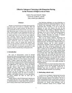
1.2.1 Natural Subspaces Within a 3-dimensional iteration space with axes, i, j and k, each reference and each operation has a natural subspace which is a subspace of this iteration space. A subspace is a subset of the set of indices in the iteration space. An index in the iteration space, say i, is in the natural subspace of a reference or an expression if, for dierent values of i, the value of the expression or reference may vary. As shown in Figure 1-1 there are eight distinct subspaces for a 3-dimensional iteration space, fi; j; k g. They are fg, fig, fj g, fk g, fi; j g, fi; k g, fj; k g and fi; j; k g. Consider the following loop nest. do i = 1, imax do j = 1, jmax do k = 1, kmax a(...)

= b(k) + c(i)

enddo enddo enddo

21

{i,k}

{j}

{j,k}

{k}

{}

{i} {i, j}

Figure 1-1: Natural Subspaces In this example, assume the subspace of the reference b(k) is fkg and the subspace of c(i) is fig. Then the subspace of the operation b(k) + c(i) is fi; kg. The natural subspace of the right hand side of this assignment is fi; kg regardless of whether the left hand side is a, a(i), a(i, k) or a(j, k). Natural subspace analysis will determine this. If the left hand side is not consistent with the natural subspace of the RHS, subspace analysis may alter this object (and the reference). For example, if this left hand side reference is a(i), the subspace compiler will convert it to a(i, k). The subspace algorithm determines a mapping from each reference in the source program to a reference in a new program. Given a set of dimensions in the source program, the subspace compiler may add a dimension that was not in the source (as in this example), it may remove a source dimension, or it may simply maintain a dimension from the source to the target. The algorithm for determining subspaces propagates information from one reference to another. For a avor of the propagation algorithm we reexamine the example above. As we have seen, the fact that k belongs to the subspace of the reference to b(k) on the RHS is propagated to the LHS, and means that k belongs to the subspace of the reference on the LHS. Suppose the reference on the LHS were a(j, k). If k 22

belongs to the subspace of this reference, this tells us that the second dimension of a is one that we should not remove in the transformed code. The fact that we should not remove the second dimension of a in this LHS reference is then propagated to RHS uses of a, indicating that we should not remove the second dimension of those references. This, in turn, helps in determining indices that belong to the subspace of each RHS reference. Then the propagation continues. This algorithm determines the subspace of each reference to a named variable. It also determines how each reference is transformed into a reference in the generated program.

1.2.2 Operational Subspaces Given the subspaces of all the named variables in an expression tree, the subspace of an intermediate result is simply the union of the subspaces of its operands, since if any of the operands vary as some index varies, then the result of the operation varies with that index as well. This is how we determined that the natural subspace of b(k) + c(i) was fi; k g in the example above. If the natural subspace of the + is fi; kg then the operands of the + must be in that subspace for the operation to be performed. b(k) in natural subspace fkg must be expanded across the fig axis, resulting in an object in fi; kg before the addition can take place. Similarly c(i) must be expanded across the k axis. fi; kg is called the operational subspace of these operands because they must be expanded from their natural subspace to this space to perform the operation.

1.2.3 Expansions The subspace abstraction is a two-part abstraction. In addition to the concept of subspace, the abstraction includes the concept of expansions. The expansion concerns how the values of elements of the object in some subspace become available. When an object in a given subspace is allocated storage, the values of the elements are unde ned (empty). Ultimately, the elements become de ned (full). During the computation, 23

Serial

s = func(s)

Parallel prefix

s = s + a(i)

Parallel

s(i) = a(i) + b(i)

Figure 1-2: Expansion Categories the de ned portion expands along each axis. The notion we are attempting to capture here is how (in what order and at what speed) the object lls up with values along each axis. The three possibilities, serial, parallel and parallel-pre x, are called natural expansion categories. They describe how the values expand to ll the object along an axis. A natural expansion category is associated with each index of a subspace. This expansion category Figure 1-2 shows the three potential expansion categories. Consider the object s. In all three cases s in subspace fig, assuming each statement is in a loop on i. Even though s is written as a scalar in some cases, the value varies with the index i in all three examples. In the rst case, the value of s for each value of i depends on the value of s for the previous i. This expansion must occur serially. If the extent of the i loop is imax then this expansion requires O(imax) time. In the second case the values of s depend on earlier values of s but the operation is such that a parallel-pre x expansion is possible. Here the time required is O(log(imax)). In the last example, all values 24

a)

b)

c)

Figure 1-3: Transformations based on Expansion Categories can be computed in parallel, requiring O(1) time. In these examples, the object is 1-dimensional. For multi-dimensional objects, an expansion category is determined for each axis in its natural subspace. A 3dimensional object may, for example, expand along two dimensions in parallel and along the last via a parallel-pre x expansion. Also notice that for serial and parallelpre x expansions, more than one object may be involved in an expansion, if, for example, t(i) is de ned in terms of s(i) which is de ned in terms of t(i) for the previous i. Loop nest a in Figure 1-3 shows two perfectly nested serial loops with six operations within them. The indices are not speci ed. As a result of expansion analysis, loop nest a might be converted to the loop nest b. The rst thing to notice here is that the subspaces of the operations have not been altered. Each operation in nest a is doubly nested. Each operation in b is also doubly nested. Next notice that some computations that were serial along some index in a have some degree of parallelism in b. Also a given serial loop may be converted to several distinct loops, each with 25

possibly dierent expansion categories. Expansion determination uncovers loop level parallelism (both parallel and parallelpre x). The system also uncovers non-loop parallelism. In fact, what the subspace compiler generates is not b but rather c which indicates the partial orderings among fragments of code of various granularities from ne-grain instruction level to coarsegrain task level. In c we see that the two outer level loops from b can run concurrently. Within the rst (left) outer loop, the two inner loops can run concurrently. And nally, within the second (right) loop, the two operations can run concurrently. To summarize, the two aspects of the subspace abstraction are the natural subspace of an object and, for each index in the natural subspace of an object, the natural expansion category of that index. One way to understand this approach is that it distinguishes between two types of communication at the subspace level. 

Expansion to natural subspace Communication is required to determine the value of an element from a previous element in the same object. This is due to a serial or parallel-pre x expansions described above.



Expansion to operational subspace Communication is required when an object in its natural subspace is expanded to its operational subspace. If an object in subspace fig is added to an object in subspace fi; j g the object in fig must be expanded across fj g for the operation to be performed.

The subspace level communications are determined by the subspace compiler. They are inherent in the computation itself. They are not an artifact of the con guration (i. e., the number of processors or the arrangement of the processors) of the target. The subspace level communications are used as input to the data and code layout phase to help determine layout. The layout generated determines actual communication of three types. 26



Expansion to natural subspace An axis with subspace level communication caused by an expansion to natural subspace will require actual communication if it is at least partially distributed across the processors.



Expansion to operational subspace An axis with subspace level communication caused by an expansion to operational subspace will require actual communication if it is at least partially distributed across the processors.



Alignment Actual communication may be required to align two objects within the same subspace. If an object in subspace fi; j g is added to another object in subspace fi; j g, communication may be necessary if, as a result of layout decisions, corresponding elements of these objects do not reside in the same processor. This type of communication is totally outside the realm of subspace analysis and only comes into being as a result of layout.

1.3 Subspace Analysis in the Context of Full Compilation This section addresses how subspace compilation ts in to a heavily optimizing targetspeci c parallel compiler. Such compilers, the Rice Fortran D compiler and the Stanford SUIF compiler for example, are typically divided into a front, middle and back as follows. 

The front handles parsing, semantic analysis, and classical scalar optimizations.



The middle performs target-speci c parallel optimizations. These include interchanging loops to move parallelism inward or outward depending on the target 27

architecture, tiling to maximize locality, data layout, code layout and scheduling. 

The back emits code for individual processors. It either emits scalar source code which is subsequently compiled or it emits machine code directly.

Basically the front is target independent, the middle is based on the type and con guration of parallelism available and the back is based on the processor instruction set. At a high level, all subspace processing (subspace analysis, expansion analysis, optional subspace optimizations, intermediates and restructuring) t between the front and middle. Although this subspace processing assumes a parallel target, it is independent of the type of parallelism. At a lower level, of course, there are a few details. The choice of scalar optimizations is modi ed by the existence of subspace analysis. (See Appendix A for details.) The existence of subspace analysis changes the way we think about the middle of the compiler. 

Some transformations in the middle are no longer required. For example, privatization and parallelization are subsumed by subspace analysis.



Some of the algorithms in the middle may generate better results because the improved input to these algorithms increases their options. For example, axes that were not explicit in the input are now available to data and code layout algorithms for distribution.



Some of the algorithms in the middle can be simpli ed because of the intermediate form subspace analysis emits. Each array and each operation is in is natural subspace. Each operation is within its appropriate expansions. Potential for concurrency is explicit.



Some of the algorithms in the middle can be improved by having them use cost information available as a result of subspace analysis. The distinction among 28

serial, parallel and parallel-pre x computation is now explicit as are expansions to operational subspace. Subspace analysis transforms the code to a form in which each reference is in its natural subspace and its natural expansions. One concern that may arise is that this approach may actually cause ineciency by being overly aggressive in uncovering axes and in distinguishing among fragments. The concern is that we may actually be increasing memory requirements or incurring excessive overhead. But subspace analysis simply uncovers potential. It passes on the transformed code with all the potential exposed to downstream target-speci c analyses. If the potential is not used in some case, the target-speci c compiler is free to undo any transformation performed here. Let's examine the three cases: natural subspaces, operational subspaces and fragmentation. 

Natural Subspaces The concern here is that adding an axis to an object may increase memory requirements. The transformed program may no longer t in the available space or, even if it ts, it may make more references deeper into the memory hierarchy degrading performance. Subspace analysis provides the information that values vary along some axis, possibly one that was missing in the source. Subsequent transformation phases may make use of that information for some target by distributing that axis intelligently. If the downstream analyses determine that the values along that axis are all local to a processor, then there is no reason to actually expand the axis in the generated code. If the axis is partially distributed, for example 128 values per processor across 64 processors, then the axis is partially expanded, one element in each of 64 processor where that one element takes on 128 successive values. The extent of the axis in the generated code is determined by its distribution. The process of eliminating axes that are not useful will occur downstream from the subspace compiler because it depends on the results of target-speci c analyses. This elimination process need not be cognizant of whether an axis was 29

visible in the source or was the result of our analyses. Therefore axis elimination may well eliminate (partially or totally) some axes that were explicit in the original source. In this case, it is even possible that the resulting code may use less memory than the original. 

Operational Subspaces Expansions to operational subspace may raise similar concerns about memory. Consider a distributed memory machine performing the operation b(i) + c(i,j) described above. Assume that after subspace analysis, the layout phases determine that the i axis of c will be distributed but the j axis will be serialized. Actually expanding b to its operational subspace is not only unnecessary, it will require execution time and will increase memory requirements. This expansion, inserted during the subspace analysis, enables the layout phases to accurately account for the time and space required for various layouts. But if the j axis is not distributed, there is no reason to actually perform the expansion. The requirement is that a value of b(i) is available on each processor that uses it. If c is partially distributed across the j axis, say 128 elements to a processor, then b is partially expanded as well requiring one element per processor (not one element per value of j). In fact, this distinction in costs enters into the layout decision.



Fragmentation Another concern may be that this model fragments the code into chunks that are smaller than necessary, resulting in unnecessary ineciency. Again, these transformations are for analysis purposes only. Two distinct fragments can be later combined by target-speci c phases. For example, if subspace analysis generates two distinct fragments because one is in fig and the other is in fi; j g, we may want to combine them if the j axis is serialized (stored within the memory of a given processor as opposed to across processors). Consider two fragments that are distinct because their expansions are independent. If the target-speci c layout decisions in the back-end cannot take advantage of the 30

potential concurrency uncovered between them, it is free to combine them to reduce overhead. In conclusion, where the potential uncovered by the subspace model can not be exploited by the target, the subspace transformations can be reversed. The apparent ineciencies are not actually incurred.

1.4 Contributions This section identi es the two claims concerning the subspace model that we will defend for this thesis. The Primary Claim is: The notion of shape is central to many optimizations, strategies and language concepts for parallel systems. The subspace model uni es, generalizes, simpli es and improves a variety of these shape-related approaches. We will show, for example, that the subspace model 

improves and uni es two parallel models, one that focuses on data distribution and the other that focuses on code distribution.



uni es and generalizes invariant code motion and privatization.



improves the SPMD strategies: owner-computes and the replication of scalars.



provides more exibility to data layout, code layout and VLIW scheduling.

These improvements result in a cleaner and simpler compiler. All the usual software engineering bene ts accrue throughout all phases of the software life-cycle. The Secondary Claim is: The subspace model is an architecture-independent parallelism analysis. Loop parallelism is uncovered by the subspace compiler as a direct result of determining subspaces and expansions. Non-loop parallelism is uncovered by the partial ordering of fragments both within loop bodies and at the top level. 31

Subspace compilation is not directed at any particular architecture. It does not include target-speci c transformations to maximize the type of parallelism handled by a speci c target. Following the subspace compiler, downstream analyses determine how the application's available parallelism can best be mapped to the particular target architecture. For example, the subspace model may determine which loops in a generated loop nest are parallel, parallel-pre x and serial. The target-speci c transformations for SIMD and vector systems will attempt to move the parallel loops inward while the target-speci c transformations for SMPs will attempt to move the parallel loops outward. The discussion under the primary claim focussed on software engineering gains within a given compiler for a single target. For the secondary claim, the improvements accrue between distinct compilers for distinct targets. In the current state-of-the-art, a programmer at an installation of a particular architecture writes a program tailored to that architecture which is then compiled by a compiler that optimizes for that architecture. Meanwhile the programmer's counterpart at an installation with a dierent architecture is working on the same application, but it must be written and compiled with a distinct target in mind. A long term goal of the subspace model is to modify this scenario. A programmer, who is savvy about parallel algorithms and about the application domain, writes a program without considering the distinction among various parallel targets. This program is compiled by a two-part compiler. Part one, the subspace compiler, deals with issues of parallelism in general, ignoring distinctions among dierent parallel targets. Part two, deals with all the issues speci c to the target at hand. A company with a product line that includes a variety of parallel architectures would then use a single subspace compiler with multiple back-ends, one for each target architecture. A user with a major application can implement it once and port it smoothly. Although there may always be certain situations (determined by both application characteristics and performance requirements) that elude these goals, we hope to widen the scope of applications that can be handled in this way, moving us closer to this ideal. 32

1.5 Organization This section presents the organization of both the compiler and the remaining chapters. The overview of the compiler structure is presented in Figure 1-4. In addition to the usual lexing, parsing, semantic analysis, and error detection, the Front-end includes conversion of the code to static single assignment form. The two major analyses in the subspace compiler, subspace analysis and expansion analysis, determine the subspaces and expansions for named references. These are presented in Chapters 2 and 3. These are together in the gure because their interaction is complex. As presented in this thesis the interaction between these two analyses is not strictly linear. But even as presented, the result is more conservative than necessary. A more aggressive solution calls for more complex interaction between these phases as described in Appendix C. The Intermediates phase determines the subspaces and expansions for intermediates from the subspaces and expansions of their operands. This phase breaks up expression trees into fragments that are consistent with respect to subspace and expansions. This allows each fragment to be executed in its appropriate subspace and with the appropriate level of parallelism. This approach also maximizes opportunities for concurrent execution of distinct fragments. Intermediate processing is addressed in Chapter 4. The restructuring phase uses tables built up during analyses to incorporate fragments in loops that correspond to their subspace and natural level of parallelism. Code fragments that form the body of a loop (or the body of the top level of the routine) are partially ordered, uncovering non-loop based parallelism. Chapter 5 describes the information collected by previous phases and shows how that information is used to generate the output of the subspace compiler. These phases, natural subspace analysis, natural expansion analysis, intermediate processing, and restructure, addressed in chapters 2 through 5, constitute the basic subspace compiler. In Chapter 6, we introduce a set of optional optimizations speci c to the subspace 33

abstraction. These are based on the results of the subspace and expansion analyses. If included, they must precede intermediate processing since one eect of these optimizations is to alter the shape of the expression trees. The Back-end might include target-speci c transformations to improve parallelism for a speci c architecture, target-speci c analyses such as data layout, code layout, and VLIW scheduling, and a full code generator. In fact, the goal is a set of Backends for a set of targets. However, for this thesis the Back-end generates Connection Machine Fortran, based on Fortran 90, to run on the CM-5. The subspace compiler does not strictly include the Back-end and nothing relevant to the subspace model occurs there so it will not be discussed further in the thesis. Chapter 7 presents some experimental results. Chapter 8 defends our primary and secondary claims. In defense of the primary claim, this chapter compares the subspace model with a variety of existing techniques. In the process, this chapter constitutes a discussion of related works as well. Chapter 9 addresses future possibilities uncovered by the subspace model. Chapter 10 concludes. Appendix A summarizes the compilation phases presented. Appendix B describes the current status of the implentation. Appendix C explains why the approach presented is overly conservative in some cases and how this could be remedied. Appendix D is a glossary of terms.

34

Front-end

Natural Subspace Analysis

Natural Expansion Analysis

Optimizations [optional] Intermediates Restructure Back-end

Figure 1-4: Compiler Design

35

36

Chapter 2 Natural Subspaces The subspace compiler will determine the natural subspace for every reference in the program. This includes references to user-declared objects and to intermediate computations. This chapter presents a global analysis which determines the natural subspace for references to user-declared objects only. Subspaces for intermediates are addressed in Chapter 4. As a result of natural subspace analysis each reference in the source is converted to a reference in the target. There are three possibilities for conversion at the dimension level. The conversion may maintain a dimension from the source to the target. It may delete a dimension from the source in the target. Or it may add a dimension to the target that was not in the source. A reference mapping is associated with each reference indicating how each reference in the source is mapped to create a target reference. The input to the natural subspace algorithm is described in Section 2.1. The natural subspace algorithm itself is presented in several steps. The core algorithm is presented in Section 2.2. It operates on a very restricted input language called the core language. Section 2.3 shows how relaxing the language restrictions impacts the algorithm. This presentation order allows us to introduce the basic terminology and the fundamental ideas while allowing us to postpone some of the complexities.

37

2.1 Input This section addresses the one restriction in the form of the input to the natural subspace algorithm. The input must be in static single assignment (SSA) form. This means that there is at most one textual assignment to each scalar [18] and to each array. This restriction is ensured by the Front-end. Conversion to SSA form occurs prior to subspace analysis. Multiple assignments are given distinct names. At merge points the names are merged via a phi operator. For example do i = 1, imax do j = 1, jmax if (bool(i,j)) then

RHS1

x(i,j) = else

RHS2

x(i,j) = endif

enddo

enddo

becomes do i = 1, imax do j = 1, jmax if (bool(i,j)) then x1(i,j) =

RHS1

else x2(i,j) = endif

RHS2

enddo

enddo x3(:, :)

= phi(bool(:,:), x1(:,:), x2(:,:))

Here x3 takes on the values of x1 or x2 depending on the associated value of bool. 38

SSA form allows us to trivially identify the single de nition associated with each use.

2.2 Core Natural Subspace Algorithm First we present the basic idea of the subspace determination algorithm. We do this by restricting the input language and presenting only those aspects of the algorithm required for this restricted input. This allows us to delay presenting some of the details until the basics are clear. This section presents the natural subspace algorithm for the core language. Section 2.2.1 speci es the core language. Section 2.2.2 introduces concepts and terminology. Section 2.2.3 describes the basic ow of the core algorithm. Section 2.2.4 presents the details of the core algorithm at a lower level.

2.2.1 Core Language Restrictions The language restrictions for the core algorithm are listed below. 

Assignment statements and do loops are the only statement types considered.



For each reference, its reaching de nition is unique and trivially determined. This is guaranteed by SSA from. Notice that for globals and arguments, the entry to the routine constitutes the single assignment. They are not rede ned within the routine and all references to them within the body of the routine are to their value on entry.



Expressions are composed of constants, scalars and arrays. Function calls are not allowed.



The following array reference restrictions hold.

{ Each subscript of an array reference is a single loop index. { Within a given array reference, a given loop index appears in at most one subscript.

39

s4 : s5 : s6 : s7 : s8 :

do i = imin, imax s = s + 1 do j = 1, jmax do k = 1, kmax a(i, j) = s * e(k) + i ... = a(i, j) ... = a(i, k) enddo ... = a(i, j) enddo enddo

Figure 2-1: Core Language Example The array references a(i), b(j,i) and c(i,k) satisfy these restrictions. The array references a(k+1), b(i+j), c(j,j) and d(i,v(j)) do not satisfy these restrictions. Notice that the question of data types is totally orthogonal to subspace and need not be restricted in any way. Section 2.3 will show how these language restrictions are relaxed.

2.2.2 Core Concepts and Terminology This section introduces the concepts and terminology needed for the core algorithm. The discussion relies heavily on the example in Figure 2-1. Assume e in that example is a global. The term named object denotes any scalar or array that is given a name in the source (s, a, e, i, and kmax). Unnamed objects are the results of computations (the result of the * or the +). An object is either a named or an unnamed object. An index is the variable controlling a loop. For example, i is an index in our example. A de nition is an occurrence of a named object on an LHS. A de nition modi es values. A reference is an occurrence of a named object on either the RHS or the LHS. In compiler literature, the term iteration space is normally assumed to be restricted according to the bounds of the iterations. Here we are not concerned at all 40

with these bounds. The axes are critical but the extents are ignored. Therefore we represent the iteration spaces simply as sets of indices. A subspace is a subset of the iteration space.

De nition 1 An index, say i, belongs to the natural subspace of a reference if the

value of the reference may vary as i varies.

Consider the space Zn with basis vectors fe ; e ; :::eng where each ei is an index in the iteration space. This set has 2n subsets. Each subset is a subspace of the iteration space. For example, objects de ned within loops on i, j and k may be in one of the eight distinct subspaces of the iteration space corresponding geometrically to the origin of the cube (fg), the axes of the cube (fig, fj g, fkg), the faces of the cube (fi; j g, fi; kg, fj; kg) and the whole cube (fi; j; kg). To avoid confusion, let's compare this with several other related concepts. 1

2



The subspace abstraction is distinct from dimensionality in that it distinguishes among, for example, the 3 dierent 2-dimensional planes that have dierent orientations.



The subspace abstraction is also distinct from the notion of a virtual processor. The notion of virtual processors is used in compilers for distributed memory systems before the restriction to the actual number of physical processor is taken into account and before the code or data distribution is analyzed. The notion of virtual processors distinguishes among dierent positions on a given axis via the details of subscript expressions. For example, x(i), x(i+1), x(i*2), x(sin(i)) and x(v(i)) are considered to be in distinct virtual processors, but they are all in subspace fig.



The subspace abstraction as used here is slightly more abstract than the normal de nition of iteration space (or subspace of the iteration space) in that we do not consider an axis to be restricted by an upper or lower bound. The axis is either part of the subspace or not. A subspace is therefore simply a set of indices not a set of points in a multi-dimensional space. 41

The subspace compiler will transform the source code to target code, the architectureindependent output of the subspace compiler. As a result of the natural subspace algorithm, the set of objects in the source will be transformed to a dierent set of objects in the target. The references to these objects will be transformed accordingly. The transformations we allow include only the following three possibilities: 

A dimension of the source may be maintained in the target. The subscript in the target will be identical to that in the source.



A dimension in the source may be deleted.



A dimension not in the source may be added in the target. Such a dimension will be subscripted by a loop index (not a function of a loop index) in the target.

A dimension appearing in the source is a source dimension. Source dimensions are either maintained source dimensions or deleted source dimensions. A dimension not appearing in the source but added to the target is called an added dimension. The reference mapping notation indicates the relationship between a reference in the source and the associated reference in the target. A reference mapping is associated with each reference since the mapping may be dierent for distinct references of the same source object. The form of the reference mapping is < SA > where S and A are sublists of source and added dimensions respectively. Elements of A are enclosed in square brackets to distinguish them from elements of S . An element in S or A indicates the disposition of the associated dimension. Each is a set of indices called potentially contributing indices. In addition, each element in S or A may be attributed as a contributing dimension. These related notions of potentially contributing indices and contributing dimension are discussed below.

De nition 2 An index i belongs to the set of potentially contributing indices of a

dimension, d, of a reference, if modifying the value of i may modify the value of the subscript expression at d.

The potentially contributing indices of a dimension of a reference are those indices in the natural subspace of the subscript expression for that dimension. Notice that 42

in the core language, since a subscript is simply an index, the natural subspace of the subscript is available immediately by inspection. For example, in Figure 2-1, S for the reference to a in statement s6 is < fig; fj g > indicating that the rst dimension potentially contributes i and the second dimension potentially contributes j. If the set of potentially contributing indices is a singleton set it may be represented without the enclosing curly braces. < fig; fj g > may be expressed as < i; j >. Although for the core language, the potentially contributing indices are available by inspection, this will not always the case when the restrictions are relaxed. Consider a reference a(s, k), where s is a scalar but not an index. The potentially contributing indices of the rst dimension cannot be determined by inspection. (See Section 2.3.1.4 for further details.) Each element in the list A is a single index because each added dimension is associated with a single index. For example, in Figure 2-1, A for the LHS reference to a in s5 might be [k] indicating that the reference has an added dimension, k. The indices of A are always ordered in canonical order according to the loop depth of the associated loops. In addition, a dimension (and its associated position in either S or A) may or may not be attributed as a contributing dimension.

De nition 3 A dimension in a reference is a contributing dimension if it contributes to the subspace of the reference.

A dimension contributes to the subspace if changing the value of the subscript in that dimension possibly alters the value of the reference. If i and j are loop indices in a reference x(i, j) with natural subspace fig, the value of the reference varies as i varies but not as j varies. In this case, as we vary the subscript in the rst dimension, say from x(12, 5) to x(13, 5), the value of the reference may change. However, as we vary the subscript in the second dimension, say from x(12, 5) to x(12, 6), the value of the reference does not change. Therefore, the rst dimension is a contributing dimension but the second dimension is not. A contributing dimension 43

is indicated in the reference mapping by underlining. The reference mapping for x is therefore < i; j >. Added dimensions may also be contributing. If s in s4 has a contributing added dimension on i then its reference mapping would be < [i] >.

De nition 4 The contributing indices of a dimension are de ned as follows: 

If d is a contributing dimension, then the contributing indices of d are the potentially contributing indices.



If d is not a contributing dimension, then the contributing indices of d are the empty set, fg.

Consider the reference, x(i, j, 3). The initial reference mappings show the potentially contributing indices would be < i; j; fg >. Suppose the rst and third dimensions are actually contributing. This is indicated in the modi ed reference mapping < i; j; fg >. This results in the contributing indices for each dimension indicated in the reference mappings < i; fg; fg >.

De nition 5 The contributing indices of a reference are the union of the contributing

indices of all the dimensions in S and A.

The contributing indices of a reference with reference mapping < i; j; fg; [k] > are fi; k g. Each contributing dimension of a LHS object will become a dimension of the generated target object.

2.2.3 Core Algorithm: High level Description Now we can introduce the algorithm to determine a subspace for each textual occurrence of a named object when the source is restricted to the core language. Brie y, after an initialization phase, the algorithm propagates indices from the RHS of an assignment to determine the subspace of the LHS. The indices of the subspace of the LHS determine the contributing dimensions of the LHS object, that is, 44

the reference mapping. The contributing dimensions of the LHS object are propagated to determine the subspace of RHS references to that object. This propagation continues until there are no further changes. The algorithm is executed in worklist style. A reference is inserted onto the worklist when its current state changes. A reference is pulled o the worklist to propagate its change. No particular order of processing, such as inner loops rst, is necessary. An index, i, belongs to the natural subspace of a reference if its value may vary as i varies. There are two distinct ways that this may occur. 

Via cyclic expansion: The object is de ned in terms of itself (either directly or indirectly) in a previous iteration of the i loop.



Via propagation: The object is de ned in terms of some reference which has i in its natural subspace.

Indices involved in cyclic expansions are uncovered in the process of discovering the expansion categories (see Chapter 3). Such indices are simply incorporated directly at initialization as we see in section 2.2.3.1. The remainder of this chapter focuses on how we add indices to subspaces via propagation.

2.2.3.1 Initial Information Before we describe how information is propagated, we begin by identifying what is known before propagation begins. 

Constants are in the null subspace since they do not vary with any index. For example, the constant 7 in a RHS expression is in subspace fg.



Loop indices are in their own subspace. Consider the expression a(i) + j, in loops on i and j. The term j is known initially to be in subspace fj g. 45



All potentially contributing indices can be determined by inspection. Note that this is due to the array reference restrictions in force for the core algorithm and is not true in general. In a(i, j) the potentially contributing indices are fig for the rst dimension and fj g for the second dimension. This results in an initial reference mapping for this reference of < i; j >.



For each reference to a global or an argument, all source dimensions are contributing and there are no added dimensions. Based on the core language restrictions (see Section 2.2.1), all references to globals and arguments refer to the object available at routine entry. Based on the conservative assumption that all the elements in the array as declared may have been assigned distinct values by the calling routine, we must assume that all the source dimensions are contributing. According to these restrictions, these objects are not de ned within the routine. Since added dimensions only arise from de nitions within loops, this restriction implies that there are no added dimensions. A reference a(i, j) where a is a global or an argument is given the reference mapping < i; j >.



For each object that is part of a cycle based on index, i, as determined by expansion category analysis (See section 3.1.1), that object has i in its subspace. Consider the examples below. do i = imin, imax

do i = imin, imax

s = s + 1

s = func(s)

...

...

= s ...

enddo

= s ...

enddo

In these examples, the rst assignment de nes s as a function of s on a previous iteration of the loop. This means that it may have a distinct value for each i and therefore has i in its subspace. The reference to s in the second assignment 46

is there simply to indicate that we might want to refer to the interim values, not just the end result. If the cycle were longer, say s is de ned in terms of t which is de ned in terms of s, both s and t would include i in their subspaces. Objects in cycles must be included explicitly at the start of the algorithm. The propagations discussed below will not uncover i as part of the subspace in the examples above, even though they will in the following case: do i = 1, imax s = s + a(i) ...

= s ...

enddo

2.2.3.2 Propagation within Assignments In brief, the subspace of the LHS object is determined by the subspace of the RHS expression. The subspace of the LHS is used to determine which dimensions of the LHS are contributing dimensions. This is explained in more detail below. Subspace: If an index, i, is part of the subspace of one of the references on the RHS of an assignment, then it is part of the subspace of the LHS object. In other words if, as i varies, the value of the RHS may vary then we will ensure that the LHS object will be generated in such a way as to have an axis associated with varying i. In the assignment, c = d(i+1, j) * e(i), if the RHS is in subspace fi; j g, then c is also in subspace fi; j g. These two indices may be propagated to the LHS one at a time in either order. Regardless of whether the LHS in the source were written as c, c(i), c(i,j) or c(i,k), its natural subspace will be fi; j g upon termination. Reference mapping: The reference mapping for an LHS reference speci es the mapping of the LHS source object to a generated subspace object. This mapping is determined by the indices in the subspace of the LHS object. If an index, i, is part of the subspace of the LHS and if i is a potentially contributing index for a dimension then that dimension is a contributing dimension. The core language restriction that 47

within a given array reference, a given loop index appears in at most one subscript implies that there is at most one dimension that potentially contributes i. If i is not a potentially contributing index for any dimension then an added dimension based on i is created. Consider the LHS, a(i, j). The reference mapping begins as < i; j > indicating the potentially contributing indices, no contributing dimensions and no added dimensions. When the index i is added to the subspace of this LHS reference, the rst dimension becomes a contributing dimension and the reference mapping becomes < i; j >. When the index k is added to the subspace, an added dimension is added and the reference mapping becomes < i; j; [k] >. If the algorithm terminates without adding j, the nal subspace for this reference is fi; kg with reference mapping < i; j; [k] >.

2.2.3.3 Propagation across Assignments In brief, the contributing dimensions of the LHS of an assignment propagate through a dependence to determine the contributing dimensions of an RHS reference. The contributing dimensions of an RHS reference determine its natural subspace. This is explained in more detail below. The situation is slightly dierent for source dimensions and for added dimensions so we discuss them separately. 

For each contributing dimension, d, that is a source dimension of an LHS

Reference mapping: If dimension, d, in an LHS reference is contributing, then dimension d contributes in any RHS reference reached via a true dependence.

In our example in Figure 2-1, assume the reference mapping for the LHS of s5 is < i; j; [k] >. When propagating from the LHS to an RHS, for source dimensions, it is the positions of the contributing dimensions that are relevant. We then transfer these contributing dimensions by position through the dependences to the RHS references in both s6 and s7 to indicate that the rst dimension in 48

both of these references is contributing. The third dimension is not a source dimension.

Subspace: If a dimension of a reference is contributing, the potentially con-

tributing indices of that dimension are in the subspace of the reference.

If the rst dimension of the RHS reference in s6 is contributing, the potentially contributing indices in that dimension, i, actually contribute to the subspace. i is therefore in the subspace of the RHS reference in s6. 

For each added dimension of an LHS

Reference mapping: If there is a true dependence from some LHS reference,

L, to an RHS, R, and there is an added dimension on index, i, associated with L, then that added index is transferred to R exactly when R is within the loop i.

The LHS reference to a in s5 has reference mapping < i; j; [k] >, with an added dimension on k. This reference reaches three RHS references, in s6, s7 and s8. The contributing added dimension on k propagates to both s6 and s7. However, since the reference in s8 is not within the loop on k, the added dimension on k cannot be propagated there. The reference mapping for s8 includes an added dimension on [kmax]. Since kmax is a scalar, this dimension has no potentially contributing indices.

Subspace: An added dimension contributes its index to the subspace. The reference mapping,< i; j; [k] >, for the reference to a in s6 indicates that this reference is in subspace fi; kg whereas the reference mapping for the reference in s8 is < i; j; [kmax] > and therefore in subspace fig. Figure 2-2 shows our example program indicating nal reference mappings as they will be determined by this algorithm. 49

s4 : s5 : s6 : s7 : s8 :

do i = imin, imax s = s + 1 = + do j = 1, jmax do k = 1, kmax a(i, j) = s * e(k) + i = * ... = a(i, j) ... = ... = a(i, k) ... = enddo ... = a(i, j)

< [i] >

< [i] >

< i; j; [k] > < [i] > < k > + < i > < i; j; [k] >

< i; k; [k] >

< i; j; [kmax] >

enddo enddo

Figure 2-2: Core Language Example with Reference Mappings

2.2.4 Core Algorithm The high level structure of this core algorithm is found in Figure 2-3. The algorithm is a worklist algorithm. Assertions about what is known are put on the worklist. When these assertions on the worklist are processed further assertions become known. Recall from section 2.2.3 that an index is determined to be part of a subspace in two ways: cyclic expansion and propagation. The code in this gure contains four statements. The rst statement initializes the worklist with assertions known via cyclic expansion. The next two initialize the worklist with assertions known at the start of the propagation algorithm. The last one begins the propagation algorithm. This high level describes the insertion and deletion of assertions in the worklist. The actual eect of these assertions is described in Figure 2-4. The access routines for the program graph and the reference mappings used in these two gures are described in Figure 2-5. One of the two types of assertions corresponds to the propagation from RHS to LHS within a statement. The other corresponds to propagation from LHS to RHS through dependences. These two items are mutually recursive. 50

LHS reference (LHS-ref) that de nes an object that is in a cycle based on an index (i) Add to the worklist:

For each

index-is-in-LHS-subspace(LHS-ref,i)

RHS reference (RHS-ref) to a global dimension (d) in RHS-ref Add to the worklist:

For each For each

dimension-of-RHS-contributes(RHS-ref,d)

RHS reference (RHS-ref) that is an index (i) Add to the worklist:

For each

index-is-in-LHS-subspace(get-LHS-ref(RHS-ref),i)

(worklist is not empty) Remove and execute any item on the worklist Figure 2-3: Main Routine

While

The assertion index-is-in-LHS-subspace is the result of a propagation of an index from the RHS to the LHS of an assignment. The impact of this assertion (the result of processing this item when it is removed from the worklist) is to nd the dimension of the left hand side reference, LHS-ref, that potentially contributes index, i. Given the array reference core language restrictions there is at most one such dimension. If there is no source dimension that potentially contributes i, then an added dimension on i is created. In either case, the result is that a dimension in the LHS-ref is determined to contribute. The assertion dimension-of-RHS-contributes is the result of a propagation of a contributing dimension from the LHS through a true dependence to a RHS. The impact of this assertion (the result of processing this item when it is removed from the worklist) is to determine the index that is contributed by this dimension and asserting that that index is in the subspace of the associated left hand side.

2.2.5 Core Algorithm: Analysis This section addresses complexity and termination of the natural subspace determination algorithm. 51

 index-is-in-LHS-subspace(LHS-ref,i) If i

)

(there is a source dimension (d) of LHS-ref whose subscript is a function of mark-as-contributing(LHS-ref,d) For each RHS-ref get-RHS-ref-list(LHS-ref) If is-contributing?(RHS-ref,d)

RHS reference (

) in

not Add to the worklist:

dimension-of-RHS-contributes(RHS-ref,d)

Endif Else If

not is-added?(LHS-ref,i)

mark-as-contributing( LHS-ref, add-dimension-on-index(LHS-ref,i)) For each RHS-ref get-RHS-ref-list(LHS-ref) If RHS-ref i

RHS reference ( ) in ( is within the scope of the loop) Add to the worklist:

dimension-of-RHS-contributes(RHS-ref,d)

Else add-dimension-on-index(RHS-ref,last(i))) Endif Endif Endif

 dimension-of-RHS-contributes(RHS-ref,d) mark-as-contributing(RHS-ref,d)

Add to the worklist:

index-is-in-LHS-subspace( get-LHS-ref(RHS-ref), find-contributing-indices(RHS-ref,d))

Figure 2-4: Worklist Items

52

 get-LHS-ref(RHS-ref)

This function returns the left hand side reference associated with a particular right hand side reference, RHS-ref.

 get-RHS-ref-list(LHS-ref)

This function returns a list of right hand side references that are reached through a true dependence from LHS-ref.

 find-contributing-indices(RHS-ref,d)

This function nds the contributing indices of a dimension, d, of a right hand side reference, RHS-ref. The array reference language restrictions in the core algorithm imply that this routine returns either the empty set or a singleton set in the core algorithm.

 add-dimension-on-index(ref,i)

This function modi es the reference mapping for ref by adding a dimension on index, i, in canonical order to the list of added indices and returns that dimension.

 is-added?(ref,i)

This boolean function indicates whether there is currently an added dimension based on index i in reference ref.

 mark-as-contributing(ref,d)

This routine modi es the reference mapping for dimension, d, of ref by marking it as contributing.

 is-contributing?(ref,d)

This boolean function indicates whether dimension, d of reference ref is marked as contributing.

 last(i)

This function returns the last iteration of the i loop to be executed. For the core language this is the upper bound speci ed by the do statement. Figure 2-5: Access Routines

53

2.2.5.1 Complexity This algorithm is O(D  L) where D is the number of true dependences and L is the maximum loop depth. Consider the processing of the true dependence on x in the following code within loops on i, j and k s12 : x = ... ...

s13 : ... = ... x Suppose at some point during the propagation, fig is added to the subspace of the LHS reference in s12. If the subspace of x did not already include i then i is propagated through the dependence to the reference in s13. (This corresponds to one instance of the worklist item: dimension-of-RHS-contributes.) At some later time, fj g is added to the subspace of the LHS reference in s12 then j is propagated to the subspace of x on the RHS reference in s13. (This corresponds to a second instance of the worklist item: dimension-of-RHS-contributes.) The dependence may be processed a third time for index k. (This corresponds to a third instance of the worklist item: dimension-of-RHS-contributes.) The dependence is processed for a given index only when that index is rst added to the subspace of the left hand side. Consider the processing of a dependence to include both the propagation required from an LHS to an RHS (one instance of the worklist item: dimension-of-RHS-contributes) and from that RHS to its own LHS (one instance of the worklist item: index-is-in-LHS-subspace). In the worst case each true dependence is processed once for each enclosing loop index. Anti- and outputdependences are ignored.

2.2.5.2 Termination The algorithm is guarenteed to terminate. We add a dimension-of-RHS-contributes to the worklist only if its subspace is modi ed. This can occur only once for each loop enclosing the (single) de nition of the object as in the complexity discussion above. So the number of additions to the worklist is bounded. For each object on 54

the worklist, we propagate the added indices along each true dependence to a RHS by adding one instance of dimension-of-RHS-contributes. At most, this results in adding one instance of index-is-in-LHS-subspace. Termination is guarenteed because the number of dependences processed is bounded and the number of items added to the worklist per dependence is bounded.

2.3 Relaxing the Language Restrictions Section 2.2 addressed the natural subspace analysis with respect to the tiny core language. This section addresses the incorporation of additional language features into the model. These features include more exible array subscripting (Section 2.3.1), I/O (Section 2.3.2), intrinsics (Section 2.3.4), alternate looping constructs (Section 2.3.5) and predicates (Section 2.3.6).

2.3.1 Array Subscripts In the core language, array subscripts are restricted as follows: 

Each subscript of an array reference is a single loop index.



Within a given array reference, a given loop index appears in at most one subscript.

In this section, we show the impact of relaxing these restrictions.

2.3.1.1 Subscript may be a function of a single index and constants In the core algorithm, each subscript was a simple index. Allowing subscripts such as i + 1 and 2 * i + 3 changes nothing in the original algorithm. The function find-contributing-indices can still be performed by inspection locally. Consider a(i+1, j) = i b(j, i+3) = a(2*j, i) ...

The initial reference mappings for this example are 55

< i; j > = fig < j; i > = < j; i > Here the fact that i is in the subspace of the RHS means that the rst dimension of a on the LHS must contribute even though the subscript is i+1 rather than i. If the rst dimension of a contributes in the rst statement then the rst dimension of a contributes in the second statement. This implies that j is in the subspace of the RHS reference to a even though the subscript is 2*j rather than j. If j is in the subspace of the RHS, it is in the subspace of the LHS which implies that the rst dimension of b contributes. The nal reference mappings are

< i; j > = fig < j; i > = < j; i >

2.3.1.2 Subscripts on the RHS may include more than one index Here we allow subscripts such as (i + j) or (2*i + j) in a RHS reference. Such a dimension has multiple potential contributing indices. Consider a(i, j) = fig ...

= a(i + j, k)

The notation on the RHS of the rst assignment simply refers to an arbitrary expression in subspace fig. The initial reference mappings for this example are

< i; j > = fig ... = < fi; j g; k > The rst dimension of the RHS reference has a set of potential contributing indices that contains more than one index. When such a dimension becomes a contributing dimension all potentially contributing indices become contributing indices and must be added to the subspace of the RHS reference. From there they will all propagate 56

to the LHS. The routine find-contributing-indices(RHS-ref,d) may now return multiple indices. The de nition of the worklist item: dimension-of-RHS-contributes(RHS-ref,d)

is modi ed to mark-as-contributing(RHS-ref,d)

index, (i) in find-contributing-indices(RHS-ref,d) Add to the worklist:

For each

index-is-in-LHS-subspace(get-LHS-ref(RHS-ref),i)

The reference mappings that result from the example above are: < i; j > = fig fi, jg = < fi; j g; k > We will maintain the language restriction that for LHS references, at most one index may be involved in a given subscript.

2.3.1.3 A given index may appear in more than one subscript Here we allow a given index to appear in more than one subscript for a given reference. The issues are slightly dierent for the RHS and the LHS. 

For a RHS reference Consider x(i, j) = ... ...

= x(i, i) ...

We will determine the contributing dimensions of the RHS reference to x in the normal way. Assume there are no added dimensions. The contributing dimensions will propagate to an RHS. If the rst dimension of the RHS reference is contributing, then i is in its subspace. If the second dimension is contributing, i is in its subspace. If both are contributing, then the de nition de nes 57

a 2-dimensional object but the reference is only referring to a 1-dimensional object, the diagonal. The subspace of this reference is the union of the indices contributed by all the contributing dimensions: i. 

For LHS references If a given index may appear in more than one subscript of an LHS reference, when we ask for the dimension that contributes some index, there may be more than one. Recall that on the LHS at most a single index is involved in a given subscript. The system will simply choose one. This will be a contributing dimension. The other will not. Given the static single assignment requirement, the LHS in question is the only assignment to the object. Consider a(i, i+1, j) = ...

within loops on i and j. The only values de ned are those whose rst two dimensions have the stated xed relationship to each other. Given one subscript, the other is determined. RHS references to that object may only refer to elements whose subscripts conform to this relationship. Otherwise the reference is to unde ned elements. Therefore, in a semantically correct program, the RHS reference may be a(i, i+1, ...), a(i-1, i, ...), a(5, 6, ...) or a(j, j+1, ...) but not a(i, j, ...). In other words, the index contributed by the RHS will be the same regardless of which dimension on the LHS was chosen as contributing.

2.3.1.4 Subscripts may be objects other than loop indices In the core algorithm, we associated a reference mapping with each array but not with subscripts. These were not necessary since the only allowable subscript was an index and the potentially contributing indices for such a subscript are trivially available by inspection. When we allowed expressions involving constants or even 58

multiple indices, the potentially contributing indices were still trivially available by inspection. But a subscript may be a reference to an object whose subspace is not available by inspection. Such subscripts require reference mappings. Consider s = ... x(...,...) ...

= ...

= x(s, i+1)

in loops on i and j, where s is a scalar but not a loop index. Here the subspace of the subscript, s, in the rst dimension of x, is not available by inspection so it requires a reference mapping. The Reference mappings actually return values. The value of a reference mapping is the set of contributing indices it indicates. There are four possibilities for the subspace of s: fg, fig, fj g, or fi; j g. During the propagation algorithm, s used as a subscript is handled just like any other RHS reference to s with respect to receiving indices in its subspace. And the rst dimension of x is handled just like any other dimension in a RHS reference with respect to determining that it is a contributing dimension. If the subspace of s is fully known by the time the rst dimension of x is determined to be contributing, this is processed just like the case where the potentially contributing indices are known. That is, if the subspace of s is known to be fi; j g, when the rst dimension of x is determined to contribute, we can propagate i and j to the LHS as for the core algorithm. The issue is that there are two requirements for a dimension, d, of an array to contribute an index, i. 

Dimension, d, must be a contributing dimension and



Index, i, must be a potentially contributing index of dimension d.

Since the potentially contributing indices are no longer trivially available by inspection but require propagation, these pieces of information can arrive in any order. For example, if the algorithm 1. rst discovers that i is in the subspace of s then 59

2. discovers that the rst dimension of x is contributing, and nally 3. discovers that j is in the subspace of s. The reference mappings at each step are: 1. < ; i > where  is not a simple index but rather the reference mapping < [i] > 2. < ; i > where is not a simple index but rather the reference mapping < [i] > 3. < ; i > where is the reference mapping < [i]; [j] > Since the reference mappings return sets of indices, these are equivalent to 1. < ; i > where  is < [i] > 2. < i; i > 3. < fi; j g; i > Therefore we can propagate i to the LHS at step 2 and we can propagate j to the LHS at step 3. This language feature raises one additional concern about the correctness of the algorithm. In the core algorithm, information, once discovered, could propagate immediately. Here, the subspace of a subscript is not available immediately by inspection. For example, to propagate i to the LHS in the example above, we need to know 1. i belongs to the subspace of s. 2. The rst dimension of x in the RHS reference contributes. 60

We might be concerned that the propagation gets stuck in such a way that, although i really is in the subspace of the LHS, i never propagates to the LHS because propagation to this LHS is exactly what enables us to determine either 1 or 2 above. But notice that if this is true, then there is a path in the dependence graph as follows: (assume the LHS in question is a de nition of y.) (LHS def of y) ! (RHS ref to y) ! ... (LHS def of s or LHS def of x) ! (RHS ref to x(s, ...)) ! (LHS def of y) But such a path constitutes a cycle. i will be added to the subspace on the basis of this cycle during the algorithm's initialization phase.

2.3.2 I/O I/O statements are easily incorporated into the natural subspace computations. Input statements act as de nitions of objects and output statements act as references. Consider the read statement do i = ... do j = ... do k = ... read x(j) ... enddo enddo enddo

The x(j) clearly may have a distinct value for each value of i, j and k. The reference mapping is therefore < j; [i]; [k] > and acts just like a de nition of x with respect to the rest of the algorithm. A write statement acts as a RHS reference and receives propagated information as any RHS reference. 61

2.3.3 Explicit parallelism The Fortran 90 triplet notation provides a mechanism for representing unnamed indices. For example, x(1:n) = y(2:n+1) + z(1:n)

based on a single unnamed axis is equivalent to do i = 1, n, 1 x(i) = y(i+1) + z(i) enddo

with respect to subspaces. The subspace analyzer simply generates index names in these cases and initializes these dimensions to be contributing and to potentially contribute the generated index. In other words, the reference mapping for one of the above references might be: < genindex1 >

2.3.4 Intrinsics There are a wide variety of intrinsic functions that may be called from Fortran routines. This section describes how these functions are incorporated into the subspace determination algorithm. Many intrinsics are simply unary operators from the perspective of the subspace calculation. For example, the sin function returns an object that is in exactly the same subspace as its argument. So the sin function in the rst assignment below is handled identically to the unary minus in the second statement. do i = 1, imax do j = 1, jmax s1 = sin(a(i,j)) + b(i) s2 = (- a(i, j)) + b(i) enddo enddo

62

The sin function takes a real argument and returns a real result. Other intrinsics behave identically with respect to subspaces even though the type of the argument and result may dier. aimag, for example, takes a complex argument and returns a real result. Not all intrinsics behave like unary operators with respect to subspace analysis. Let's examine some of the Fortran 90 intrinsics. Fortran 90 reduction functions such as all, sum or minval take an array and return a scalar. If they have a dim argument, the reduction occurs along a speci c dimension only. For example, do i = 1, imax do j = 1, jmax a(i,j) = fi, jg ... enddo enddo x(:)

= sum(a, dim = 1)

In this example there is a dependence between the LHS that de nes a and the reference to a outside the loop nest. Based on this dependence, the subspace analyzer determines that both dimensions at the reference are contributing dimensions. With respect to subspace determination, these two parallel dimensions behave just as if they were each speci ed by a loop construct. We therefore simply create internally generated names, say genindex1 and genindex2 for these indices. Since the eect of the sum function is to eliminate some dimensions, we do not simply propagate genindex1 and genindex2 to the subspace of the LHS. In this example, the rst dimension is eliminated. Only the second dimension, genindex2 propagates to the LHS. It is not always possible to determine the shape of the result at compile time. For example, the reshape intrinsic takes an array argument whose values specify the shape of the result. Since these values may be determined at runtime, this intrinsic is not analyzable at compile time. 63

2.3.5 Alternate looping constructs The only loops addressed in the algorithm above are do loops. Loops can also be created from while constructs, from repeat-until constructs and from backward gotos. Notice that the subspace algorithm makes no reference to loop bounds or loop counts even for do loops. In general, these quantities are symbolic. The question we do care about here is whether or not the value of some object may vary across iterations. Such variations may occur within the context of any looping construct. One major dierence between a do loop and other loops is that the do loop has a named index and that index may appear in constructs within the loop. Other looping constructs do not have a named index and therefore the associated index can not appear in a subscript expression in the body of the loop. A subspace compiler therefore simply generates an index name. Consider: while (bool) ... m = func(m) ... endwhile

The subspace compiler may generate the index, genindex1, for this example. The subspace of m is fgenindex1g because m is de ned in terms of itself in previous iterations of the loop on genindex1. genindex1 might also be in the subspace of an object not de ned in terms of itself as in the following example. while (bool) ... m = func(m) ... p = m + ... endwhile

Since p is de ned in terms of m which has genindex1 in its subspace, p will also 64

have genindex1 in its subspace. In this case However, consider

genindex1

is an added dimension.

10 continue ... m = func(m) ... p(m, ...)

= m + ...

if (bool) goto 10

Here again p will have genindex1 in its subspace. In this case however, genindex1 is associated with a source dimension, not an added dimension. Sometimes recursion is used as an alternate looping structure. Under restricted conditions recursion could be handled simply as an alternate looping construct by the subspace analyzer. But recursion can be used in more exible ways that are, at least at the current time, outside the scope of this work. Recursion will not be further addressed here. One might argue that loops formed from these alternate looping constructs are often simply convergence tests that must be computed serially. We might just as well ignore the subspace analysis for them. After all, the argument might go, subspace analysis will simply result in adding this additional index to all the objects assigned within this scope and since each iteration depends on the previous one, no additional parallelism will be found. Some reasons for actually performing subspace analysis on these loops follow: 

Some of the operations may not have the generated index in their subspace. These can be removed from the serial loop and executed just once.



Some of the operations within that loop may be parallel or parallel pre x across the generated index. These can removed from the serial loop and put in a separate parallel or parallel pre x loop.



Even if all the operations are serial in the generated index, they may be involved 65

in several distinct cycles across the generated index. This means that we may be able to improve performance by performing these distinct cycles in parallel. 

Consider the assignment a = func(a) + b(i). func and + are both computed serially. But assume that b is de ned by a parallel computation and all uses of a are parallel. A data layout phase may well decide that distributing a across i is worthwhile even though it is computed serially. This decision is in the domain of the data/code layout phase or the VLIW scheduling phase and should be based on the cost model of the target architecture. The goal of the subspace model is simply to uncover the fact that the generated index is, in fact, in the subspace of a and that a is computed serially across that index. However, the subspace analyzer is obliged to present the distribution across this index as one of many options to the data layout phase.

2.3.6 Conditional Execution Here we address the impact of conditional execution on the subspace of an assignment. We will show that an index in the subspace of a predicate aects the values of objects whose de nition is controlled by the predicate. That index is therefore in the subspace of those objects as well. In the alternate loop structures above, an if statement controlling a backward branch determined the number of consecutive iterations (possibly zero) of a loop. However, the value of de nitions within the loop did not depend on the predicate. When we consider incorporating if statements that control the execution of assignments within their scope, that situation changes. In this case, the body is executed on arbitrary, possibly non-consecutive, iterations of enclosing loops. This changes the role of the predicate in subspace calculations. A predicate itself, of course, is simply an expression and its subspace is determined as we determine the subspace for any expression. For example, consider the code 66

do i = 1, imax do j = 1, jmax if (a(i) .gt.

b(j)) then

... endif enddo enddo

If a(i) is in subspace fig and b(j) is in subspace fj g, the predicate is in subspace fi; j g. Full details of subspace determination for expressions are found in chapter 4. Since a predicate has no explicit LHS, it might seem that the propagation of subspaces would stop at the conditional expression itself. This is not true. Consider do i = 1, imax do j = 1, jmax x = s + j ...

= x ...

enddo enddo

Assume s is in subspace fg. Since the value generated by this assignment depends only on j, not on i, x is in subspace fjg. Now consider the same assignment controlled by a predicate in subspace fi, jg. do i = 1, imax do j = 1, jmax

s9 s10

if (a(i).gt.b(j)) then x = s + j endif

s11

...

= x ...

enddo enddo

The discussion of this example is illustrated in Figures 2-6, 2-7 and 2-8. The three 67

gures show the values of three objects: rst the predicate, (a(i).gt.b(j)), in statement s9, then the expression, s + j, in s10 and nally the values referenced by x in s11. These gures do not show all the values of these objects. We are only concerned with determining the values of x in s11 where j is 48, indicated by the # on the j axis and where i is 3, indicated by the ! on the i axis. The values of the predicate, as shown in Figure 2-6, vary arbitrarily, that is, both i and j are in the subspace of the conditional. For each i, j pair for which the assignment is executed, the value of x depends only on j. This means that, for a given column of the expression s + j (Figure 2-7), all values are the same since this gure indicates only those values actually evaluated. In particular, where j is 48, for iterations of the i loop where the assignment is actually evaluated, the value of the expression is 3. For i equal to one or two, for example, the value of x is 3. However, consider the value of x in statement s11 for some iteration, (i, j), for which the assignment is not executed. (3, 48) is such an iteration. Since x is not assigned on this iteration, its value on that iteration will be the value of its most recent assignment. We nd this value by looking back along the j axis in the predicate for the most recent true value (Figure 2-6). This is found three columns back at j is 45. We then inspect Figure 2-7 to nd that the value of x at iteration (3, 45) is 7. Figure 2-8 shows us the values of x for each point in the column where j is 48. Notice that it is no longer true that all the values in a given column are the same which means that it is no longer true that the values depend only on j. These values depend on i to determine the iteration, (i0, j0), in which the assignment was last executed. clearly varies as i varies so, by the de nition of subspace, i is clearly part of the subspace of x. This is true even though, whenever the assignment to x is executed, the value does not depend on i. In general, indices in the subspace of a predicate controlling an assignment to an object contribute to the subspace of the object. Predicates in if statements are incorporated into the subspace determination x

68

i

j

48#

t t 3! t f f f t t f f t t t f f t Figure 2-6: Values of the Predicate: a(i).gt.b(j)

i

j

48#

3 3

7

3!

3

5

3 3

5

3

Figure 2-7: Values of the Expression:

i

j

s + j

within the scope of the if

48#

3 3 3! 7 3 5 3 3 5 3 Figure 2-8: Values of the RHS Reference: x outside the scope of the if 69

algorithm as follows:



Each predicate that is not simply a reference to a name, is given a generated name, with the expression as its RHS. The example above becomes

do i = 1, imax do j = 1, jmax gentemp = a(i).gt.b(j) if (gentemp) then x = s + j endif enddo enddo



The named conditional controlling an assignment acts simply as an additional RHS operand in the subspace propagation algorithm.

Subspaces propagate from the de nition of a to the use of a on the RHS of the assignment to gentemp. They may propagate to the de nition of gentemp on the LHS. They may propagate to the use of gentemp in the conditional. Now, in addition, the subspace of gentemp will propagate as a use to the RHS of the assignment to x. A complete discussion of how predicates are incorporated into RHS expressions is found in Section 4.5. At this stage, it suces to know the impact of predicates on global subspace analysis. They act as RHS references in assignments they control. There is a possible optimization of predicate processing. Consider the distinction between the two examples below. 70

do i = 1, imax do j = 1, jmax if (a(i).gt.b(j)) then x = s + j endif ...

= x ...

enddo enddo do i = 1, imax do j = 1, jmax if (a(i).gt.b(j)) then x = s + j ...

= x ...

endif enddo enddo

In the rst example, the reference to x is executed on iterations where x is not de ned and the discussion above applies. However, in the second example, x is referenced only on iterations where it is actually de ned. In this case, the subspace of the predicate is not relevant. The subspace of x in this case is simply fig. For this optimization, if the references, both LHS and RHS, involve subscripting, they must be interrogated to be sure the value referenced is always de ned. Remember that the predicate processing described here only applies to predicates of if statements that control the execution of assignment statements. It does not apply to predicates of if statements that control backward gotos or predicates of while statements. These are simply alternate looping constructs. The predicates in these cases impact the number of iterations executed but not the subspace. The termination and complexity analysis above remain accurate if the term RHS is taken to include both the actual RHS of an assignment and the conditionals controlling that assignment. For example, the objects contributing to the RHS of the 71

assignment to x above are s, i and gentemp. Note that this may signi cantly increase the number of true dependences indicated in the complexity measure.

2.3.7 Calling with Accurate Arguments So far we have only shown the processing for leaf routines since we have not yet included the processing for function or procedure calls. First, we will assume no interprocedural analysis. This implies that the shape of objects visible between calls are not aected by subspace analysis. The processing for the core language assumes that the incoming arguments and globals are as declared in the source. We must ensure this on the calling side. There are two possible problems 

There is a dimension in an argument that we have removed.



There is a dimension in an argument that we have added.

The rst can be dealt with simply by a replication. The user-declared x as two dimensional and calls user-func(x(:,:)). We determine that only the rst dimension contributes. x is converted in the transformed program to x1 which is 1-dimensional. This implies that all the values along the removed axis are identical. The called routine expects a 2-dimensional argument. This is an example of an operand in a subspace that is smaller than required by its operation. As usual, this situation requires an expansion across operational subspace. The second case is more interesting. The user-declared x as two dimensional. We transform this to x2, a 3-dimensional object with an added dimension across k. To process a call to user-func(x) we must convert this to user-func(x2(:,:,current-k)) which passes all elements along the rst and second axes but only the current slice along the k axis. 72

2.3.8 Returning Modi ed Arguments One of the language restrictions we included as part of the static single assignment is that globals and arguments are not modi ed. Essentially their only assignment is from outside the routine. Sometimes however, we need to actually modify these values. We relax this restriction simply by allowing a block of assignments to these objects immediately prior to return. These assignments cannot reach any use in the routine and do not participate in the subspace analysis.

2.4 Summary The subspace analysis presented in this chapter determines which loop indices aect the value of each reference, both RHS and LHS, to each user-declared object. It uses this information to transform the shape of the objects to ensure that distinct values (assigned in distinct iterations of some loop) are written to distinct elements in the object. Notice that the program started in static single assignment form so an object, say x, is modi ed by only one assignment. We then transform the program so that if the assigned values vary with some index, say i, then i is a subscript of some dimension of x in the assignment, for example, x(...,i,...) = .... The program is now dynamic single assignment at the element level, that is, during execution of the program each element is assigned to at most once. This form eliminates both anti- and output-dependences. Since these dependences restrict reorderings, this new from simpli es downstream analyses.

73

74

Chapter 3 Natural Expansions The subspace abstraction includes two notions: the subspace of an object, addressed in Chapter 2, and how the values of elements of the object become available with respect to the subspace, the topic of this chapter. When an object in a given subspace is allocated storage, the values of the elements are unde ned (empty). Ultimately, the values of all the elements are determined (full). During the computation, more and more of the values become de ned. The notion we are attempting to capture here is how (in what order and at what speed) the object lls up with values. A natural expansion category is associated with each index of a subspace. This expansion category describes how the values expand to ll the object along an axis. Notice that expansion as used here is not to be confused with the term scalar expansion. Scalar expansion refers to the compilation process of taking a scalar variable supplied by the user and converting it (expanding it) to an array object in the generated code. (This is an added dimension in our terminology.) We use the term expansion to refer to a runtime phenomenon occurring within an object of xed size. Expansions should not be confused with dynamically allocated objects that expand (actually increase in size) at runtime. Here the object is already allocated and it is simply a question of the evaluation order of the elements within the object. Consider an object de ned within a nest of three loops. If the source code is scalar, it appears that the object lls up (expands) with values serially through the three loops, evaluating one element at a time. But in the same way that we determine 75

the natural subspace by analysis, instead of taking the subspace to be that given in the source, we will also determine the natural expansion category by analysis instead of assuming it is given by the source. Expansion analysis may determine that as a result of the outer loop, one dimension of the object expands serially; as a result of the middle loop, another dimension of the object expands in parallel; and as a result of the inner loop a third dimension of the object expands via a parallel-pre x operation. (See Chapter 1 and Figure 8-1 for an introduction to these three expansion categories.) Expansion analysis is applied to every axis in the runtime object, regardless of whether the axis was declared in the source or uncovered by natural subspace determination. We have said that these expansion categories capture the notion of how (in what order and at what speed) the object lls up with values. They are called to as natural expansion categories in that the speed and order referred to here are not those on any speci c target architecture but rather those that arise directly as a consequence of the computation itself. Section 3.1 introduces the basic idea of expansions. Section 3.2 presents the algorithm that identi es expansions and determines their categories. These ideas are presented with respect to the limited language of do loops and assignment statements. Section 3.3 shows how additional language constructs are incorporated into this algorithm. Section 3.4 discusses the integration of subspace analysis and expansion category analysis within the compiler.

3.1 Concepts and Terminology One way to view expansion analysis is as a generalization of privatization. When an object, s, is privatized [37, 44] along a loop index, i, two things happen. The object is given an additional dimension subscripted by i and the de nition of s is asserted to be parallelizable along that dimension. We extend this notion in two ways. 

First, we analyze all the indices in the natural subspace of this object. We are not limited to those that were missing in the source. 76



Second, we determine which one of three expansion categories is the natural expansion category for each axis. We are not limited to parallel expansions.

The idea is introduced via a restricted language that includes only do loops and assignments. Below we introduce the three natural expansion categories. The examples are for both source and added dimensions. 1



Parallel - the value of each element along an axis is not based (either directly or indirectly) on previous elements along that axis. The anticipated communication costs are O(1) for parallel axes. s is expanded in parallel across i in both examples that follow. do i = 1, imax ...

do i = 1, imax

= s

...

= s(i-1)

s = x * y(i)

s(i) = x * y(i)

...

...

= s

enddo

= s(i)

enddo

Our de nition of parallel is similar to that used for privatization but diers in two important ways. First, it does not require that all references to an element be in the same loop iteration as long as the de nition of an element does not depend on previous elements along that axis. In the rst statement, the use of s de ned on the previous iteration does not prevent the i axis from having a parallel expansion category though it would prevent the object from being privatized. In addition, as mentioned above, it applies to existing source dimensions as well as to added dimensions (dimensions added by subspace analysis). The identi cation of an axis as parallel does not mean that the operations along that axis will be performed \at the same time". For example, if the values of y are not available all at the same time, then, on some targets, they can be used as they become available. 1 This is not as restrictive as the core language described in 2.2.1 for subspace analysis. In particular, the restrictions on subscripts do not apply here.

77



Serial - the value of an element is potentially based on the value of elements earlier along that axis. The anticipated communication costs are O(N ) where N is the extent of the axis. s in the following code is serially expanded across i. do i = 1, imax

do i = 1, imax

s = userfunc(s)

s(i) = userfunc(s(i-1))

enddo



enddo

Parallel-pre x - the value of an element is based on the value of elements earlier along that axis but the operations can be converted to parallel-pre x form with communication cost of O(log N ). s in the following code is a parallel-pre x expansion across i. do i = 1, imax

do i = 1, imax

s = s + b(i)

s(i) = s(i-1) + b(i)

enddo

enddo

The examples above are simpli ed in that in each, the axis in question corresponds to the innermost loop. In fact, an expansion category is determined for each index. In the following code, s is in subspace fi; j g and is parallel-pre x along j but parallel along i. do i = 1, imax s = 0 do j = 1, jmax s = s + b(i, j) enddo enddo

3.1.1 Cyclic Expansions For the serial and parallel-pre x expansions in the examples above, there is a cycle of nodes involving a loop-independent dependence from an LHS to an RHS and a 78

loop-carried dependence from that RHS to the LHS within the same statement. The term cyclic expansion refers to an expansion that is either serial or parallel-pre x. A given cycle may involve more than one object and more than one statement as in do i = 1, imax x(i) = y(i-1) + b(i) y(i) = x(i) + c(i) enddo

In fact, we do not distinguish between distinct cycles if they are strongly connected. Consider do i = 1, imax x(i) = y(i-1) + z(i-1) y(i) = x(i) * b(i) z(i) = x(i) * c(i) enddo

This code has one cycle between x and y and another cycle between x and z. Since the goal is to keep all statements involved in both cycles as part of the same cyclic loop, we will focus on nding strongly connected components (SCCs) as opposed to cycles. We do, however, distinguish between distinct SCCs. For example, consider do i = 1, imax x(i) = y(i-1) + a(i) y(i) = x(i) * b(i) z(i) = z(i-1) * c(i) f(i) = z(i) + x(i) g(i) = f(i) * 2*i enddo

We will uncover two SCCs, one de ning x and y, and another de ning z. Each of these is called an expansion. So x and y are part of the same expansion while z is part of another. These distinct expansions might have the same or dierent 79

expansion categories. f and g are not part of any SCC and are therefore distinct parallel expansions. This information will allow the restructuring phase (see Chapter 5) to generate the following loops. 2

do i = 1, imax x(i) = ... y(i) = ... enddo do i = 1, imax z(i) = ... enddo do i = 1, imax f(...)

= ...

enddo do i = 1, imax g(...)

= ...

enddo

The rst two loops will be cyclic. The last two will be parallel. A cyclic expansion is a set of assignments together with an index. In static single assignment form, this is equivalent to a set of objects with an index, since each object is associated with exactly one assignment. We therefore identify a cyclic expansion by the index and one of the objects in the set. An expansion is written as (object ! index), for example, (x ! i), which is read as \the expansion of x across i". If the expansion contains more than one object, we choose a representative object for its identi cation since each object may be part of at most one expansion with respect to a given index. Notice, however, that the same object will be part of an expansion, possibly a cyclic one, with respect to each index in its subspace. So x may well be part of one expansion, say (x ! i), across i and some other expansion, say 2

The ordering among these loops is determined by the restructuring phase.

80

(y ! j ), across j. This notation does not distinguish between serial and parallelpre x expansions. In fact, we use the same notation to indicate a parallel expansion. The expansions above are (x ! i), (z ! i), (f ! i), (g ! i). At this point we can summarize the goals for expansion analysis as follows: 

to determine the natural expansion category of each loop we generate. A parallel loop is more ecient than a parallel-pre x loop which is in turn more ecient than a serial loop.



to isolate separable components of a loop into distinct loops, so that some loops can be performed via more ecient expansion categories. A loop containing both a serial expansion and a parallel expansion must be performed serially. But, if separated into two distinct loops, one can be performed in parallel.



to isolate separable components of a loop into distinct loops so that even if these components are performed via the same expansion categories, they can be performed concurrently. A single loop containing two distinct SCCs both of which are serial might be faster run as two distinct, serial loops run concurrently.

3.1.2 LHS and RHS References Consider a cyclic expansion (b ! i). The eect of this expansion is to ll in values along the i axis of b. We must now determine which dimension of b corresponds to the i axis. The reference mapping for the LHS of the assignment to b indicates which dimension contributes i. If the reference mapping for the LHS reference de ning b is < i; j; [k] >, the expansion (b ! i) will ll in values along the rst dimension of the generated object. If the reference mapping is < k; j; [i] > it will ll in values in the third dimension of the generated object, an added dimension in this case. By focusing on the LHS references, the process appears to be at the assignment statement level which is at odds with our general expression level philosophy. Now we 81

address RHS references in order to support expression level analysis. (See Chapter 4 for a discussion about expansions of intermediates.) Consider do i = imin, imax

s1 : s2 :

a(i) = a(i-1) + b(i) * ... ...

= a(i)

enddo

Here the two references to a in s1 are in an SCC on i, (a ! i). However, neither the reference to b in S 1 nor the reference to a in s2 are part of that SCC. The use of a in s2 can be separated into a distinct expansion and accessed in a parallel loop if appropriate for its operation. In fact, the * in s1 can also be separated and performed in parallel. It is easy to confuse the role of the index and the role of a dimension when discussing cyclic expansions. The expansion is represented with reference to the index, say as (a ! i), because the expansion loop iterates over this index but the eect of the expansion is to ll in values along a speci c dimension. The importance of this distinction was not that clear when we were looking at an LHS reference because the relevant dimension was the one which contributed the relevant index. But notice that this is not necessarily true for a RHS reference within cyclic expansion. Assume s1 in the example above is replaced by s3 in the example below. s3 : a(i) = a(k) + b(i) * ... Here a cyclic expansion, (a ! i), expands a across the rst dimension. The RHS reference to a is part of that expansion (assuming apparent dependences). But i is not even a potentially contributing index of the rst dimension of the RHS reference. In fact, i does not even belong to the subspace of the RHS reference. The speci c expansion identi ed with an index is associated with a speci c dimension and propagates from an LHS through a dependence to the same dimension of an RHS. This positional aspect to cycles is similar in avor to the positional aspect of contributing dimensions of RHS references in subspace analysis. This example raises an interesting issue which we refer to as the subspace of a 82

dependence addressed in Appendix C.

3.1.3 Loop Nests So far we have considered only the innermost loop. Once we have analyzed the innermost loop, we will examine the loop enclosing it. This section examines issues relevant to processing multiple loops in a loop nest. Consider the two loops in the two cases below do i = ...

do i = ...

x = z ...

y = z ...

do j = ...

do j = ...

a = b + x ...

a = b + x ...

b = a + y ...

b = a + y ...

enddo

enddo

z = b ...

z = a ...

enddo

enddo

Assume each named reference is subscripted so that all RHS references have dependences to the appropriate LHS de nitions. In each case we rst process the inner loop on j and discover the cyclic expansion (a ! j ) that includes a and b. We process the i loop after completion of the j loop. During i loop processing, we consider the loop-carried dependences on i and loop-independent dependences. In the example on the left, we nd a cycle that includes x, a, b and z. This is a correct expansion. However, the example on the right has a problem. There is no path from the y reference on the RHS to the a reference on the LHS without following the loop carried dependence on j. But, on the other hand, if we simply include all the loop carried dependences on j we will nd the cycle that includes a and b. But we already knew there was a cycle here from our previous processing of the index j. The solution is to collapse the cyclic expansion, (a ! j ), to a single composite assignment. This composite assignment includes all the RHS references in the cyclic expansion as RHS references of the composite and includes all the LHS references in the cyclic expansion as LHS references of the composite assignment. Dependences 83

between the composite assignment and other assignments remain but those within the composite are suppressed. So in the graph for nding SCCs for index i, we can reach any LHS reference from any RHS reference but this path does not appear to contain any cycles. While processing the index i, the graph for example above on the right is as if produced from a program like the one below. do i = ... y = z ...

fa, bg = fa, b, x, y, ...g z = a ... enddo

3.2 The Algorithm Here we present the algorithm for expansion analysis. The top level structure is /* Locate cyclic (parallel-pre x or serial) as opposed to acyclic (parallel) references */ For each source loop index, index, in post-order Find all the SCCs with respect to index Collapse each SCC into a composite assignment /* Distinguish parallel-pre x from serial references */ For each SCC, S, Determine if S is parallel-pre x or serial Add entry to SCC table that includes identi er index set of objects expansion category Annotate each named reference that is part of S as belonging to S 84

/* References that are not cyclic are parallel */ For each object, obj For each index, index, in the subspace of obj If obj is not expanded cyclically over index Annotate it as parallel The distinction between serial and parallel-pre x expansions depends on the detection of recurrences. See [11, 9, 22] for more on parallel-pre x computations. We now address the location of SCCs. The analysis of the SCCs with respect to a given loop, say i, begins with the graph whose nodes are the program nodes within the i loop. The edges among these nodes include 

the expression tree edges



the loop-independent dependence edges



the loop-carried dependence edges that are carried by the i loop



the control dependence edges

We then apply an SCC algorithm [16] to this graph, recording all references, RHS and LHS, that belong to this SCC as part of the same cyclic expansion. Since each loop is processed once and for a given loop, the algorithm to determine the SCCs terminates, this algorithm terminates. The SCCs algorithm is linear in the size of the graph (V+E). We apply this algorithm to the body of each loop. Since each element of the program graph is processed via at most one SCC algorithm for each loop enclosing it, the algorithm is O(L  N ) where L is the maximum loop depth and N is the size of the whole program graph.

3.3 Relaxing the Language Restrictions The previous discussion focussed on determining expansions for the restricted language of do loops and assignments. This section shows how predicates and I/O are 85

incorporated into expansion analysis.

3.3.1 Predicates Here we consider the addition of conditionals (structured if statements). We have already seen that predicates aect the subspace of objects (see Section 2.3.6). Predicates can also aect expansions by creating cycles. Consider the following example do i = 1, imax

s3 :

if (b.eq.

...)

then

do j = 1, jmax

s4 : s5 :

if (a .gt.

...)

b = t(...)

then

+ u(...)

...

s6 :

a = y(...)

+ z(...)

endif enddo endif enddo

Here the value of a in s4 depends on the assignment to a in s6 via a data dependence. But the value of a in s6 depends on the predicate in s4 via a control dependence. These two dependences create a cycle within the j loop. To incorporate predicates into the expansion analysis, we therefore require control dependence edges in the graph. Notice that b is involved in a cycle on i but cannot be part of a cycle on j since the cycle is broken when the only nodes considered are within the loop on j.

3.3.2 I/O I/O operations can also be incorporated into the natural expansion analysis. Input statements act as de nitions of objects and output statements act as references. Unlike de nitions via assignment, input statements have no RHS objects. However, they 86

may be involved in cycles as in the following example do i = 1, imax if (a ...)

then

read x endif a = x ... enddo

Output statements can not cause cycles. Notice that expansion analysis uncovers information that would be useful in determining when parallel I/O would be eective.

3.4 Phase Integration The expansion analysis as presented in this chapter appears to be totally independent of the subspaces algorithm presented in Chapter 2. One might assume that we know the indices in a subspace before we determine the expansions over these indices. However, this is not necessary. Expansion analysis uncovers references that participate in cycles over an index, say i. We don't need to know before expansion analysis that i is part of a subspace of an object. But if that object is involved in a cycle on i, we can conclude, as a result of expansion analysis, that i belongs to its subspace. Performing expansion analysis before the subspace analysis will enable us to initialize the subspace calculation (see Section 2.2.3.1) with objects expanded cyclically. Some of these cases are outside the realm of the subspace propagation. For example, consider s = s + 1 in a loop on i. Subspace propagation alone will never uncover that i is in the subspace of s. However, expansion analysis will discover the cycle and will determine that i is in the subspace of s. A cycle across an index means that the value may vary along that index, and that that index is part of the subspace. With this in mind, execution order for the subspace compiler is as shown in Figure 1-4. As with most interesting compiler work, however, we nd that the interaction 87

index, index, in pre-order Find the SCCs with respect to index. Use the SCCs to initialize the subspace algorithm. Complete the subspace algorithm. Given the subspaces and the SCCs, determine all the expansion categories. Figure 3-1: Integration of Expansion and Subspace Analyses

For each

among phases is complex. A further discussion of this topic is found in Appendix C.

3.5 Summary This chapter presented the analysis to determine the expansions associated with each dimension of each object and to isolate distinct expansions. An object may expand along an axis via serial, parallel-pre x or parallel expansions. An object may expand dierently across each axis. The expansion of some object may bound with the expansion of some other object. A loop that includes several de nitions may be transformed into several distinct expansions. This approach removes as much as possible from each loop, optimizes the loop type supporting each expansion and maximizes potential concurrency among distinct expansions. This chapter also addressed the relationship between subspace analysis and expansion analysis and identi ed some issues that complicate that relationship. The approach presented here has the same avor as parallelization algorithms, but is dierent in several ways. Its focus is on expansions of objects rather than on parallelization of loops. It is performed in the context of natural subspace analysis which alters some of the considerations. Its goal is not statement level but expression level analysis and, in fact, expression level optimization.

88

Chapter 4 Intermediates We have shown algorithms for determining subspaces and expansions for references to named objects in the program. This chapter discusses issues relating to these attributes for unnamed objects, i.e., the results of intermediate arithmetic expressions. This ner-grained analysis enables transformations at the expression level. Expressions will be computed in their appropriate subspace not necessarily the subspace of their LHS. This minimizes the computation and communication required. Expressions will be computed as part of appropriate expansions, not necessarily the expansions of their LHS. This minimizes the computations within cycles, moving some of these computations to parallel computations. We show here how the natural subspace of an intermediate is computed locally from the natural subspace of its operands (Section 4.1), assuming that global subspace analysis has already determined the natural subspace of each named reference. The natural subspace of an operand may be dierent from the natural subspace of an operation it participates in. This results in an inconsistency which must be reconciled (Section 4.2). We show here that the expansions of an intermediate are determined locally from the expansions of its operands (Section 4.4) assuming that global expansion analysis has already determined the assignments that participate in each expansion. For example, in the assignment a(i) = a(i-1) + (b(i) * s), the + is part of the cyclic expansion (a ! i) but the * is not. 89

We begin by assuming a language of assignments and do loops, but predicates in if statements are incorporated smoothly (Section 4.5). The expansions and subspaces of intermediates are used to fragment expressions (Section 4.6) so that the fragments can later be executed in the appropriate subspaces and expansions.

4.1 Natural Subspace of Intermediates Recall that the subspace of an LHS reference is determined by the subspace of the RHS references used to compute it. For example, if the subspace of x(i) is fig and the subspace of y(j) is fj g then the subspace of a in a = x(i) * y(j)

is fi; j g with reference mapping < [i]; [j] >. In the same way the subspace of an intermediate is determined by the subspace of the operands (children) that compute it. Therefore the subspace of the result of the * in a = b(i, j, k) + x(i) * y(j)

is also fi; j g. Since there is no distinction between source and added dimensions for intermediates, we simply write the reference mapping as < i; j >. The subspace of the + is the union of the subspaces of its operands, one of which is itself an intermediate. The computation of subspaces for intermediates follows the global natural subspace analysis. The local analysis is simply a bottom-up walk of each expression tree which sets the subspace of each intermediate to be the union of the subspaces of its operands. We could have chosen to incorporate the subspace determination for intermediates directly into the global natural subspace algorithm. In such an integrated algorithm, when an index becomes part of the subspace of an operand, it propagates to the subspace of the operation that uses that operand. Instead of propagating directly to the LHS, it propagates through the expression tree step by step ultimately reaching the LHS. However, there are two reasons we choose to separate the local natural subspace analysis for intermediates from the global natural subspace analysis for named objects. 90



To keep the compiler design clean especially in the presence of expression reordering optimizations. In chapter 6, we present some optimizations involving expression reordering. In performing these optimizations, we compute the subspaces of the intermediates for a variety of orderings. Reordering does not impact the propagation of subspaces from an RHS to an LHS but may invalidate work done to determine subspaces for intermediates.



To minimize the cost of the global natural subspace computation. Incorporating each index of each operand of an operation individually into the subspace of the operation can be more expensive than performing the union of sets of indices of its operands only once. This improves the design even if expression reordering were not an issue.

4.2 Operational Subspace of Intermediates Operations occur between two operands of the same subspace. Corresponding elements are combined to produce a result. In the expression tree in Figure 4-1, consider the operation a(i) + b(j) in loops on i and j. Assume that the natural subspace of a(i) is fig and the natural subspace of b(j) is fj g then the + operation occurs in its natural subspace fi; j g. Therefore a and b must both be made available in subspace fi; j g before the operation can be performed.

De nition 6 The operational subspace of an operand is the subspace of the operation

in which it is involved.

Since the subspace of an operation is the union of the subspaces of its operands, the natural subspace of an object is always a subset of its operational subspace. The expansion from natural subspace to operational subspace is always simply a replication of existing values and can be performed via a parallel-pre x operation in logarithmic time. Note that this is distinct from an expansion across natural subspace whose expansion category depends on the computation involved. 91

{i, j} +

a(i)

b(j)

{i} {j}

Figure 4-1: Operational Subspace The explicit expansion to operational subspace applies to all machines that exploit spatial (not just hierarchical) memory locality including distributed memory systems with both separate address spaces and shared address spaces (NUMA machines). The expansion to operational subspace is always performed on NUMA systems whether or not it is explicitly represented in the compiler. One advantage to explicitly representing this as an expansion is so that it can bene t from compiler optimization. In addition to the obvious optimizations, it turns out that the expansion may be redundant even when the speci cs of the communications involved are slightly dierent. This optimization is addressed in chapter 6. At rst glance, expansions to operational subspace would not seem to apply to uniform memory access machines in which all processors can access all memory locations with equal cost (UMA machines). But even on UMA machines, expansions to operational subspace might be bene cial in reducing contention. We will simply assume expansion to operational subspace applies to some, but not all targets. In this thesis, we will not look at the bene t of performing it on some but not all uses within a target. This discussion only applies to expansions to operational subspace. Expansions to natural subspace apply to all these machines. 92

+

{i} -> j, k

a(i)

*

b(j) {j} -> k

{i, j, k} {j, k} -> i c(k) {k} -> j

a) Normal distribution +

+

{i, j, k}

{i} -> j, k

a(i)

*

j {i, j, k}

{i} -> j, k

{i, j, k}

{i, j, k}

a(i)

*

j

k {i, j, k}

{j, k}

{j, k} -> i k {j, k}

c) Implicit distribution: Minimal computation

b) Implicit distribution: Minimal communication

Figure 4-2: Implicitly Distributed Objects

4.3 Implicitly Distributed Objects Some expressions can be computed locally (without communication cost) in any space that is a superset of the expression's natural space. Although the natural subspace of a constant is in the empty subspace, it is available in any subspace without communication cost. In the expression a(i, j) + 1, 1 does not require communication to expand to its operational subspace fi; j g. Similarly, in the expression a(i, j) + i, the term i is available in any subspace containing i, without communication. In particular, it is available in fi; j g, its operational space.

De nition 7 Any object whose operational subspace is larger than its natural sub-

space but is available without communication in that larger subspace is implicitly distributed since it need not be distributed explicitly. Not just leaves of expression trees such as constants and indices, but intermediates that are functions of constants and indices, e.g., i + j*2, may be implicitly 93

distributed. An intermediate is implicitly distributed if all its operands are implicitly distributed. Consider Figure 4-2. Expression tree 4-2:a shows a normal expression with three operands, a(i), b(j) and c(k) in subspaces fig, fj g and fkg respectively. Here the usual rules apply. The multiplication is in subspace fj; kg. The sum is in fi; j; kg and all operands require explicit expansion to their operational subspace. The next two expression trees are both for the expression: a(i) + (j * k)

The shapes of these expression trees and the subspaces for the leaves are identical to those in expression tree 4-2:a. However, the multiplication can now be implicitly distributed. To minimize communication, we perform the multiply and the sum in fi; j; kg as shown in expression tree 4-2:b. No communication is required. To process implicit distribution in the compiler, during the bottom-up walk of the expression trees that determines subspaces of intermediates, we keep track of nodes that are implicitly distributed, i. e., those whose children are implicitly distributed, and delay the determination of their subspaces. In Figure 4-2:b, j and k are implicitly distributed. So the * is determined to be implicitly distributed. The + is not implicitly distributed because of its left operand. In a subsequent top-down walk, at a node that is not implicitly distributed but that has at least one child that is, the subspace of each implicitly distributed child is determined to be the subspace of its parent. The * in Figure 4-2:b is therefore determined to be in subspace fi; j; kg. Once the subspace of an implicitly distributed node is determined, this subspace is propagated down its entire subtree. This propagates subspace fi; j; kg to operands j and k. Unfortunately, this approach performs more operations (in this case, more multiplies by a factor of the extent of the i loop) than is really required. On most current systems this is not as critical as minimizing communication. But if this is a critical issue for the target system, we could determine the subspace for each operation in the normal way so that no operation is performed in a subspace that is larger than 94

necessary. This approach is shown in expression tree 4-2:c. Notice that the result of the multiply must be explicitly distributed to its operational space in this case. But the leaves of the expression tree can still be implicitly distributed. This still saves an expansion of j across the k axis and an expansion of k across the j axis but minimizes computation at the cost of some communication.

4.4 Expansions of Intermediates Each LHS and RHS reference is associated with an expansion for each index in its subspace. Global expansion analysis determines these expansions for each named reference in each assignment. Suppose, for example, the LHS of some assignment is in a cyclic expansion across index i, and that some but not all of the RHS references in the assignment are part of that cyclic expansion. In such a case, some but not all of the intermediate operations may be part of the cyclic expansion. Intermediate operations that are not part of a cyclic expansion along some axis can be removed from the cyclic expansion and can be computed in parallel along that axis. We will now show how the expansions of an intermediate are determined from the expansions of its operands. A cyclic expansion identi ed by global expansion analysis must include a reference on both the RHS and the LHS. Consider the following example. do i = 1, imax a = 0 do j = 1, jmax a = a + c(i, j) * d(i, j) enddo enddo

Here global expansion analysis determines that the LHS reference is part of two expansions (a ! j ) and (a ! i). The rst is cyclic. The second is parallel. Both references to a in the inner loop are part of the cyclic expansion, (a ! j ). The other 95

references are not part of any cyclic expansion. An intermediate is part of a cyclic expansion if and only if any of its children are. This means that the + operation is part of the cyclic expansion (a ! j ). All other axes and other references are separable and parallel. In particular, the * can be computed in parallel across both i and j. The loops that result from restructuring this code are do-parallel i = 1, imax do-parallel j = 1, jmax temp(i, j) = c(i, j) * d(i, j) enddo enddo do-parallel i = 1, imax a(i,0) = 0 enddo do-parallel i = 1, imax do-parallel-prefix j = 1, jmax a(i, j) = a(i-1, j) + temp(i, j) enddo enddo

Local propagation of expansions for intermediates is not incorporated into the global expansion propagation algorithm in order to keep the compiler design clean in the presence of expression reordering optimizations.

4.5 Incorporating Predicates Recall that predicates impact the subspace of named objects, as addressed in Section 2.3.6. Predicates impact the expansions of named objects as addressed in Section 3.3.1. These discussions of predicates were at the assignment level. At that level we indicated that a predicate was processed as part of the RHS of an assignment. This section addresses how the impact of predicates actually shows up at the level of 96

individual operations within the statement. Here, since we will distinguish among distinct operations on the RHS, we need a more detailed discussion of exactly how predicates are incorporated. A predicate is treated as a binary operation on a boolean and an arbitrary object. Where the boolean is true the result is the value of the object. Where the boolean is false the result is a reserved value, NIX. NIX combined in any way with any value returns NIX. Predicates in this model behave much like where statements in Fortran 90, like masks in intrinsics, also in Fortran 90, or like context bits in SIMD systems. This handling of predicates facilitates their use in these systems but we use them also for MIMD and VLIW targets as well. Chapter 6 addresses the reordering of expressions in order to optimize with respect to subspace and expansion category. In the absence of reordering optimizations, we will simply apply the predicate at the point of the assignment, that is, at the root of the expression tree. Consider if (a(i) .gt.

b(j)) then

x(i, j, k) = c(i, j, k) + d(i, j) endif

This code will be converted to temp(i, j) = a(i) .gt.

b(j)

x(i, j, k) = temp(i, j, k) ?

(c(i, j, k) + d(i, j)) :

NIX

endif

In this formulation, the ? operator is simply an intermediate that takes two operands, a boolean object and an arithmetic object (the NIX is assumed). The previous discussion of subspaces, expansions, operational subspaces and implicit distribution apply to all operators including this one. 97

4.6 Fragmentation Fragmentation breaks up the expression trees when the expression is inconsistent with respect to either subspaces or expansions. Prior to fragmentation, the named references and the intermediates in each assignment have been annotated with subspaces and expansions. The goal of fragmentation is to break expression trees into smaller expression trees with the following properties. 

All assignments are either normal assignments or expansions to operational subspace (assignments with a RHS that is a single named reference, replicated across one or more axes).



All normal assignments are consistent with respect to subspaces. An assignment is consistent with respect to subspaces if all the named references and all the intermediates have the same subspace. This subspace is called the subspace of the assignment.



All normal assignments are consistent with respect to expansions. An assignment is consistent with respect to expansions if all the intermediates are members of the same expansions. These are called the expansions of the assignment.

These consistency goals are not always achievable. (See the discussion of subspaces of dependences in Appendix C.) Fragmentation due to inconsistent subspaces and fragmentation due to inconsistent expansions are addressed in separate sections below.

4.6.1 Inconsistent Subspaces Fragmentation will break o a subtree of an expression tree where the subspaces are inconsistent. This allows subexpressions to be performed in subspaces that are smaller than the subspace of the LHS. Consider 98

x(i) = y(i) - s

If the subspaces of the leaves are the obvious ones, the subspace of the - is fig. Since the subspace of the s in this statement is fg, this statement is inconsistent with respect to subspaces. Fragmentation will generate temp-i(i) = spread(s across i) ; expand from fg to fig and ; in fig space

x(i) = y(i) - temp-i(i)

Now consider a(i, j) = b(i, j) + (c(i) * d(i))

If the subspaces of the leaves are the obvious ones, the subspace of the + is fi; j g and the subspace of the * is fig. The * is a child of the + in the expression tree. We break the expression tree at the point of inconsistency, and add the expansion to operational space. Unless the object in the smaller subspace is a leaf, it must be named. An assignment is added to name it. If the object in the smaller subspace is a leaf, the name given it by the user is adequate. In this example, fragmentation creates temp-i(i) = c(i) * d(i) ; in subspace fig temp-ij(i,j) = spread(temp-i across j)

; expand from fig to fi; j g

and a(i, j) = b(i, j) + temp-ij(i,j)

; in subspace fi; j g

4.6.2 Inconsistent Expansions Another reason to break up an existing expression tree is inconsistent expansions. This allows subexpressions to be computed in more eective expansions than the expansions of the LHS. Consider a(i) = a(i-1) + b(i)

99

Here, although the object b is not part of the expansion (a ! i), the + is part of that expansion. This statement is consistent with respect to expansions. however, consider a(i) = a(i-1) + (b(i) * c(i))

Here both operations are in subspace fig but the * operation is not part of any cyclic expansion whereas the + is part of (a ! i). We replace this statement with the following two statements. temp(i) = b(i) * c(i)

; expanded in parallel across i

and a(i) = a(i-1) + temp(i)

; expanded cyclically across i

4.6.3 A Distinction Between these Inconsistencies Notice that the two types of consistency described above are not totally analogous. Consider again two examples from above. do i = 1, imax

do i = 1, imax

a(i) = a(i-1) + b(i)

x(i) = y(i) - s

enddo

enddo

In the example on the right the two leaves of the RHS expression are in distinct subspaces. In the example on the left the two leaves of the RHS expression are in distinct expansions. The two situations seem analogous. However, fragmentation behaves slightly dierently in the two cases. The example on the right is inconsistent with respect to subspaces but the example on the left is not inconsistent with respect to expansions. Subspace consistency requires that all named references and intermediates are in the same subspace so for the example on the right, we will fragment the reference to s and expand it to its operational space. However, expansion consistency requires only that the intermediates are in the same expansions so the left example is consistent and will not be fragmented. 100

4.7 Algorithm for Processing Intermediates Each named reference, LHS and RHS, is associated with a reference mapping and a set of expansions it participates in. A bottom-up walk propagates subspaces, expansions and an attribute indicating whether it is implicitly distributed. This walk computes subspaces, expansions and implicit distribution for the intermediates. A top-down walk propagates subspaces for implicit distributions. In a subsequent walk, expressions are fragmented where inconsistencies (either subspace or expansion) are located. Expansions to operational subspace are generated if the inconsistency was with respect to subspaces. Names are generated where necessary. These generated names are associated with nodes in the expression tree. Expansions and subspaces for these names are determined, as usual, from their children in the expression tree. Regardless of the reason for fragmentation, when an expression is fragmented, the data structures must be updated to re ect 

the removal of the initial assignment



the addition of the new assignments



the addition of any internally generated name and the associated information about this name

4.8 Summary This chapter presented the analysis of assignments required to determine the subspace and expansions of intermediates given the subspaces and expansions of the references to user-declared objects. It also addresses the fragmentation of the assignments to create a set of fragments where each fragment consists of operations that are all within the same subspace and the same expansions. This optimizes program execution by minimizing com101

putation and communication and by maximizing parallelism. It also allows for a ner-granularity of downstream analyses.

102

Chapter 5 Restructure Previous chapters describe how we analyze the program. This chapter addresses the mechanics of using the resulting information to generate a new program. On entry to this phase, subspace and the expansion information is associated with every object, that is each named reference, and each reference to an intermediate computation. We use this information to transform the input program into a new program such that each operation is within a set of loops consistent with its natural subspace and its natural expansions. This chapter includes a description of the information used by the restructuring phase (Section 5.1), the form of the generated code (Section 5.2), and the process of using the information to generate the new program (Section 5.3).

5.1 Subspace Information This section describes the information available to the restructuring phase. This information is collected by previous phases so rst a quick summary of the previous phases. 

The natural subspace of each named reference is determined (see Chapter 2).



For each index in the natural subspace of a named reference its expansion is determined (see Chapter 3). 103



Finally, the subspaces and the expansions for intermediates are determined and the expressions are fragmented based on inconsistent subspaces and inconsistent expansions (see Chapter 4).

The information available from these analyses follows. Figure 5-1 shows an example of these structures. 

Objects: a set of named objects and for each such object: { Assignment: the assignment that de nes it, that is, its static single assignment

{ Expansions: the expansion associated with each index in the subspace of this object



Expansions: a set of expansions and for each expansion: { Index: the loop index { Rep: the representative object for this expansion. This object is one of

the objects de ned by this expansion. { Xcat: the expansion category, parallel, parallel-pre x or serial. { Objects: the set of objects de ned by the expansion. Given SSA form, each object implies one assignment. If the expansion category is parallel the representative object will be the only object in the set. Parallel-pre x and serial expansions may include multiple objects. Access to the expansions is by index. 

Assignments: A set of assignments and for each assignment: { Map: each named and unnamed reference is associated with a reference

mapping which indicates the subspace. { Expansions: each named and unnamed reference is associated with a set of expansions of which it is part. There will be one expansion for each index in its subspace. 104

Objects

Expansions

A: Assignments:

B: Assignments:

Expansions:

Expansions:

i

j

(A -> j) Index: j Rep: A Xcat: Parallel Objs: ptr to A in Objects

i

(A ->i) Index: i Rep: A Xcat: Parallel-prefix Objs: ptrs to A & B in Objects

Assignments =

=

+

A(...)

B(...)

*

B(...) +

Y(...)

A(...)

2

1 Each node in these expression trees is annotated by a reference map and pointers to expansions

Figure 5-1: Subspace Information

5.2 Subspace Normal Form The restructuring phase will generate subspace normal form. This section lists the characteristics of Subspace Normal Form. 

Subspace normal form is a partial ordering of fragments where each fragment is a loop or a single operation. The body of a loop fragment is a partial ordering of fragments.



The ordering of loops in a generated loop nest is consistent with the ordering of loops in the source. However, in any given generated loop nest, some source loops may be missing and each source loop may appear multiple times in the generated code. For example, a source loop nest with nesting of indices: (i (j (k))) might generate an intermediate form with all the following nestings (i 1

2

Reordering of loops is target-speci c and so is not part of our analysis. If reordering is appropriate it will be performed after the subspace transformations presented in this thesis. 2 This notation indicates the obvious nest of three loops. The notation (x (i j) y z) would indicate three top level loops, x, y and z where loop x has two consecutive loops, i and j, nested 1

105

, , however, generate (j

,

, and (i

(j)) (i (k)) (i (j (k)) i (j)) (j (k)) (j)

.

. It could not,

i i)

(i))



Each loop is parallel, parallel-pre x or serial. Parallel loops may include multiple operations but only a single assignment. Parallel-pre x and serial loops may include multiple assignments. The operations within a given parallel-pre x or serial loop are part of the same cycle across the associated axis.



All expansions to operational subspace are explicit.

The goal is to ensure that 3



each operation is within a set of loops consistent with its natural subspace and



the expansion category of each loop is consistent with the expansion category of the operations within it.

5.3 Restructuring Before presenting the algorithm, we introduce some concepts and terminology. The restructuring algorithm is driven o of the index tree, a structure that indicates the nesting of loops. Each node in the index tree corresponds to a loop in the program. In the source, these loops were either do loops with user speci ed indices or alternate looping constructs with compiler generated indices (see Section 2.3.5). The node corresponding to the loop on index j is a child of the node corresponding to the loop on index i in the index tree if and only if the loop on j is nested inside the loop on i in the source. Consider the following source loop structure. do i1 do j1 enddo do j2

within it. 3 Appendix C discusses why current system is slightly conservative with respect to this goal.

106

do k1 enddo enddo enddo do i2 enddo

The source structure above generates the following index tree (i1 (j1 j2 (k) ) ) (i2)

The processing is performed via a post-order walk of the index tree. For the source above, post-order is j1 k j2 i1 i2

5.3.1 The Algorithm This section introduces the restructuring algorithm. We begin with a pool of assignments. This pool is simply an unordered set. We will be removing assignments from the pool and wrapping them in loops whose indices belong to the subspace of the assignment. For each index, the loop type (parallel, parallel-pre x or serial) corresponds to the expansion category of the assignment across that index. Parallel-pre x and serial loops may include more than one assignment in their body since they are formed by SCCs in the dependence graph and these components may involve more than one assignment. The process of wrapping a new loop around one or more fragments is called augmenting the fragments. Augmented fragments are returned to the pool. At any time during this process, code may be augmented by some subset (including none or all) of its required loops. Such code is referred to as a partial fragment. Code enclosed in all its required loops may also be called a completed fragment. Processing for each index completes before processing of the next begins. If the expansion category for the current expansion across index i is parallel then the relevant partial fragment is removed from the pool of partial fragments, 107

index, , in post-order of the index tree nodes expansion, exp, across ix is a cyclic expansion then the set of all partial fragments participating in exp Remove all partial fragments in PFS from the pool new-PF = augmented (partially ordered (PFS)) Throw new-PF back into the pool

For each ix For each If exp PFS =

Else PF =

the partial fragment participating in exp Remove PF from the pool new-PF = augmented (PF) Throw new-PF back into the pool

Endif Next exp Next ix completed-PFS = completed-PFS final = final

the set of all fragments remaining in the pool Remove from the pool partially ordered (completed-PFS) Throw back into the pool Figure 5-2: Restructuring Algorithm augmented by enclosing it in a parallel loop on i and returned to the pool. If the expansion category is either parallel-pre x or serial, then all the partial fragments involved in the SCC are removed from the pool, joined in a partially ordered graph indicating the ordering as required by the dependences among them, augmented by a parallel-pre x or serial loop on i and returned to the pool. Figure 5-2 presents this algorithm. The issue of joining partial fragments into a partially ordered graph is addressed in Section 5.3.3. But rst we will demonstrate the process via an example.

5.3.2 An Example Upon entry to the restructuring phase we have completed subspace analysis, expansion analysis and fragmentation. There is a pool of assignment statements each of which is consistent with respect to both subspaces and expansions. This pool might contain the following: 108

1.

a(i,j) = temp1(i,j) + temp3(i,j)

is in subspace fi; j g (a ! i) is parallel (a ! j ) is parallel

a

2.

temp = s * 2 temp

3.

is in subspace fg

temp1(i,j) = (replicate temp across fi, jg)

is in subspace fi; j g (temp1 ! i) is parallel-pre x (temp1 ! j ) is parallel-pre x

temp1

4.

temp2(i) = t(i) + para1(i)

is in subspace fig (temp2 ! i) is parallel

temp2

5.

temp3(i,j) = (replicate temp2(i) across fjg)

is in subspace fi; j g (temp3 ! i) is parallel (temp3 ! j ) is parallel-pre x

temp3

#2 is a completed fragment. If j is the inner loop then after restructuring completes processing of j, the pool of partial fragments is: 1.

do-parallel j a(i,j) = temp1(i,j) + temp3(i,j) enddo j

2.

temp = s * 2

3.

do-parallel-prefix j temp1(i,j) = (replicate temp across fi, jg) enddo j

109

4.

temp2(i) = t(i) + param1(i)

5.

do-parallel-prefix j temp3(i,j) = (replicate temp2(i) across fjg) enddo j

No additional partial fragments become complete after processing of index j. After processing index i, the pool of partial fragments is: 1.

do-parallel i do-parallel j a(i,j) = temp1(i,j) + temp3(i,j) enddo j enddo i

2.

temp = s * 2

3.

do-parallel-prefix i do-parallel-prefix j temp1(i,j) = (replicate temp across fi jg) enddo j enddo i

4.

do-parallel-prefix i temp2(i) = t(i) + param1(i) enddo i

5.

do-parallel-prefix i do-parallel-prefix j temp3(i,j) = (replicate temp2(i) across fjg) enddo j enddo i

These are all complete fragments with the following partial ordering. 110

2

4

#

#

3

5 &

.

1

5.3.3 Ordering Fragments When augmenting by a parallel loop, the body is a single partial fragment. However, when augmenting by a parallel-pre x or serial loop, the body is based on a SCC and therefore may well contain several distinct partial fragments. This section addresses the question of how to order these partial fragments within the new loop. In particular, we must show that there always exists a legitimate ordering. Source order is not always a possibility. Consider the source do i do j a = ... b = ... c = ... d = ... enddo enddo

Suppose we are about to create a serial loop on i which we have determined includes the following two distinct serial loops on j. do-serial j

do-serial j

a = ...

b = ...

d = ...

c = ...

enddo

enddo

We now want to include these two partial fragments in a single cycle within a loop in i. There are two possible total orderings of these two partial fragments. Neither 111

corresponds to source ordering. We must prove that there always is a legitimate ordering. Notice that it is not a goal of the subspace phase to create a total ordering. The subspace level of abstraction is supposed to be target- and con guration-independent. If we choose a speci c total order without taking the target and the con guration into account, we may make bad decisions for some target or con guration. Therefore our goal is to generate the partial ordering that captures the semantic requirements. To show that, during the augmentation process, we can always nd a legitimate ordering between two statements, S 1 and S 2, we must show three things. 1. In working bottom up on the index tree, these two statements begin as two separate partial fragments each of which is simply a statement with no loops. If these partial fragments are not part of the same SCC with respect to any loop, then they need never be ordered within a loop and are simply ordered at the outermost level. We need to show that, if this is the case, a partial ordering is always possible. 2. However, if at some point during the processing of an index, i, an SCC includes both statements, the two partial fragments containing these statements become part of the same (serial or parallel-pre x) loop. We need to show that when this is the case, a partial ordering is always possible. 3. An ordering set between partial fragments when they rst become part of the same partial fragment, xes that ordering for all subsequent augmentations. So we must show that this partial ordering remains acceptable through subsequent augmentations. More formally, we need to prove the following theorem.

Theorem 1 The restructuring algorithm can always nd a legitimate partial ordering of partial fragments.

The theorem follows from the following lemmas. 112

Lemma 1 There is a path in the dependence graph from any statement within a partial fragment to any other statement within the same partial fragment.

This lemma is trivially true for a partial fragment that consists of a single statement with no loops. We show that if it is true for partial fragments at some point in the restructuring process, it remains true for each new partial fragment created by augmenting existing partial fragments with an additional loop. Each time a new partial fragment is created there are two possibilities. 

It is a parallel fragment. In this case we have created a new partial fragment by added a loop around a single existing partial fragment. If the lemma held for the existing partial fragment, it holds for the new one.



It is a cyclic fragment. In this case the new partial fragment may combine several existing partial fragments. But these partial fragments were determined to be within this single cyclic fragment because they were part of an SCC in the dependence graph. So there is also a path between any two partial fragments within this cyclic fragment. We assume the lemma was true within each of these existing partial fragments. So there is a path from any statement to any other statement within the new fragment.

Lemma 2 If two fragments are not combined into any common loop during restructuring, there is always a semantically valid partial ordering between them.

We will show this by contradiction. Consider two fragments f 1 and f 2. Of the four possible partial ordering requirements between them, the only illegal one requires both f 1 < f 2 and f 2 < f 2. To show that this case cannot arise, we assume it does and show a contradiction. f 1 < f 2 implies that there is a path in the dependence graph from some statement, Sf ?s , in the fragment f 1, to some statement, Sf ?s , in the fragment f 2. Likewise 1

1

2

113

2

f 2 < f 1 implies that there is also a path from some statement, Sf ?s , in the fragment f 2, to some statement, Sf ?s , in the fragment f 1. But lemma 1 tells us that there is also a path from Sf ?s to Sf ?s and from Sf ?s to Sf ?s . These four partial paths form a dependence cycle. But a cycle among these four nodes would result in a cyclic expansion, contradicting the premise. 2

1

1

2

1

2

1

1

2

2

2

1

Lemma 3 When two partial fragments are combined to become part of a common

loop during restructuring, a semantically valid partial ordering within that loop can always be found.

First consider their ordering within a single execution of the loop being added. We only need to consider loop-independent dependences. Since there can be no cycles in this dependence graph (by an argument identical to that presented for lemma 2), the graph is a directed acyclic graph (DAG). This DAG represents a semantically valid partial ordering for code within a single iteration. Now consider the ordering across distinct iterations. These will be properly ordered if the iterations are executed in order regardless of the order of the statements within the iteration.

Lemma 4 If the bottom-up restructuring algorithm creates a partial ordering be-

tween two partial fragments when they are combined to become part of a common loop, this partial ordering remains semantically valid as this partial fragment is augmented by subsequent loops. There is a DAG, d1, of loop-independent dependences used to create the partial ordering with respect to the inner loop. There is another DAG, d2, used for the outer loop. There are two possibilities. 

d1 = d2 In this case the partial orderings are identical and the lemma holds.



d1  d2 114

In this case assume statements s1 and s2 have some partial ordering with respect to d2 that is inconsistent with their ordering when d1 is considered. Without loss of generality assume this ordering requirement with respect to d2 is s1 > s2. This implies that there is a path s1 > s3 > s2 where s3 is in d2 but not in d1. This can not be the case. When the inner loop containing s1 and s2 was created, it would have contained s3 since if s1 and s2 were in an SCC then s3 would have been included in the same SCC. This contradiction proves the lemma. Now returning to our theorem, consider two statements S 1 and S 2. There are two possibilities: 

The two share no common loops in the generated code, in which case lemma 2 applies and a partial order can be found.



They share a common loop. In this case, during restructuring, at some stage they will be merged into a single loop. At this stage, an appropriate partial ordering can be found according to lemma 3. If this is the case, the partial order for that loop will be adequate for later loops according to lemma 4.

This completes the proof of theorem 1.

5.4 Summary Previous phases annotate the named references and the intermediate operations with subspace and expansion information. The restructuring phase, described in this chapter, uses these annotations to create a new program such that each operation is within a set of loops consistent with its natural subspace and its natural expansions. This chapter described the mechanics of this process.

115

116

Chapter 6 Optimization This chapter discusses a variety of optimizations enabled by the subspace abstraction. On one hand, the subspace abstraction is distinct from scalar code. On the other hand it is also distinct from target-speci c code that might include, for example, details of code and data layout. It therefore provides a distinct opportunity. Some of the optimizations presented here are simply not available at other levels. Other optimizations use existing techniques but get dierent (better) results because they are applied at this level. Some of the optimizations presented here rely on the observation that given an expression tree, several distinct variants of that expression tree may compute the same result. Some of these variants may be more costly than others. In particular, since the subspace of an intermediate is determined by its operands, expression reordering can alter the amount of computation performed. Since the expansions of an intermediate are determined by the expansions of its operands, reordering can alter the critical path length in cyclic expansions. So uncovering the variants and choosing intelligently among them can have important rami cations for eciency. The analyses addressed in previous chapters have all been architecture- and con gurationindependent. Within this chapter identifying distinct ways of representing a computation is target- and con guration-independent but choosing among these alternatives 1

1

with a few exceptions including expansions to operational subspace and implicit distributions

117

involves target-speci c costs related to the memory system, the communication system, the extent of parallelism the target can exploit, etc. The optimizations presented here are performed after global natural subspace determination and expansion analysis since the optimizations rely on the results of these analyses. These optimizations may reorder expression trees, so they must occur prior to determining the subspace and expansions for intermediates which depend on xed expression trees. The optimizations presented here include the following: 

redundant expansion elimination (REE) REE eliminates expansions to operational subspace that are redundant. This optimization catches redundant expansions not noticed as redundant by other compilers. It replaces a replication by a reference to a previously replicated value and possibly a shift (Section 6.1).



generalized common subexpression elimination (GCSE) We view intermediate objects as in the same class as user named objects. GCSE (Section 6.2) is one optimization that arises from a reexamination of classical approaches in this new light.



a number of optimizations performed via expression reordering including:

{ minimizing subspaces of intermediates { minimizing operations within cyclic expansions { maximizing potential REEs { maximizing potential GCSEs Since xing the ordering of the expression tree xes subspaces, expansions, REEs and GCSEs, all of the optimizations must be addressed together (Section 6.3). Section 6.4 discusses how predicate processing is integrated with expression reordering. 118

6.1 Redundant Expansion Elimination Expansions to operational space are performed on NUMA systems whether or not they are explicitly represented in the compiler. One advantage of explicitly representing them is to enable optimizations on them. Existing compilers may represent these expansions at the level of speci c processor addresses. This allows them to be found redundant if the speci cs are identical. Assume the code is within loops i, j, k and m in the following examples. ...

= x(m,i,j,k) * v(i,j,k) + y(m,i,j,k) * v(i,j,k) + z(m,i,j,k) * v(i,j,k)

Assume x, y and z are all in subspace fm; i; j; kg and that v is in subspace fi; j; kg. Assume the obvious layout, with x, y and z aligned. The speci c communication to expand v to its operational subspace for each of the three multiplications will be exposed after subspace analysis and after layout analysis. Two of the three expansions can be eliminated as redundant by existing techniques after speci c communication operations are exposed. However, consider the trivial modi cation to the code above. This example below is a simpli cation of an assignment in APPLU from the NAS parallel benchmarks. This benchmark is a lower/upper triangular solver. ...

= x(m,i,j,k) * v(i+1,j,k) + y(m,i,j,k) * v(i,j+1,k) + z(m,i,j,k) * v(i,j,k+1)

With the same layout of these objects, where the objects x, y and z align, the actual communication to expand v for each of these operations will dier. So the expansion cannot be detected as redundant by existing compilers at the level of explicit communication based on a speci c layout. Nor can it be detected as redundant before these compilers make the communication explicit. The expansion is not even explicit at that point. However, we represent expansions to operational space at the intermediate level of natural and operational subspaces. At this level the communication, expressed as an abstract expansion of v across the axis m, is identical for all three 119

multiplications and is therefore redundant for two of them. At the subspace level, we expand v across m once. At the location level, we simply adjust the alignment of this expanded object by one (perform a shift) for each of the subsequent operations. Notice that the same argument would apply if the indices of v were identical but either the subscripts or the layout of z, y and x were distinct. Although this example is within a single expression and might be handled by statement-level communication optimization, this type of redundancy is more common between than within statements. The elimination of redundant expansions of an object to its operational space ignoring details of indexing and layout is called redundant expansion elimination (REE) Predicates are most likely to be improved by REE. In the subspace abstraction, predicates expand to the subspace of all the operations they control. This optimization will ensure that a predicate is actually expanded across each axis at most once.

6.2 Generalized Common Subexpression Elimination The result of an intermediate computation is an object in some subspace, but the usual common subexpression elimination algorithm is unnecessarily restrictive in that there are many recomputations of already computed elements that it is unable to detect as redundant. The problem stems from dierent treatment of named and unnamed objects. First, consider the common view of named objects.

s1 :x(i) s2 :... s3 :... s4 :...

= ... = x(i) = x(i-1) = x(j)

; in a loop on i ; in the same loop on i ; in the same loop on i ; in a subsequent loop on j

s1 is the rst (only) computation of the named object x. s2, s3 and s4 are uses of previously computed values of the named object x. 120

The four equivalent situations for unnamed objects would be:

s5 : ... = x(i) + y(i+1) ; in a loop on i s6 : ... = x(i) + y(i+1) ; in the same loop on i s7 : ... = x(i-1) + y(i) ; in the same loop on i s8 : ... = x(j) + y(j+1) ; in a subsequent loop on j s5 is the rst computation of the unnamed object formed by the +. s6 is a second computation of the same unnamed object and will be found to be redundant by the existing common subexpression elimination (CSE) technique. This technique will convert the computation in s6 to a use of a previously computed value. However, classical CSE will not notice that s7 also corresponds to a previously computed value of an unnamed object. But the distinction between s6 and s7 is exactly the same as the distinction between s2 and s3. Nor will the classical CSE technique notice that s8 corresponds to previously computed values in a distinct loop. But the distinction between s6 and s8 is exactly the distinction between s2 and s4. The generalization of CSE to handle references to unnamed objects that are not textually identical and may refer to elements computed on dierent iterations or in dierent loops is called generalized common subexpression elimination (GCSE). The key is the correct representation of the unnamed object. The CSE approach represents the unnamed object by its exact textual representation. If it is represented by the relationships among the indices and in a canonical form, it will recognize x(i) + y(i+1), x(i-1) + y(i) and even y(i) + x(i-1) as the same.

6.3 Optimization via Expression Reordering In the preceding chapters we have shown how to compute the natural subspace and the natural expansions for intermediates given xed expression trees. However, for some expressions, the same result can be computed in several dierent ways. Expressions can be reordered, for example, via commutative and associative laws, via factoring and the distributive law and, for logical expressions, via DeMorgan's law. Some orderings may be more expensive than others. 121

Recall that 

The natural subspace of an intermediate is determined from the subspaces of its children.



The expansion categories for an intermediate are determined from the expansions of its children.



Expansions to operational space depend on the natural subspace of parent and child.

For these reasons expression reordering can impact subspaces and expansions of intermediates and the expansions to operational subspace all of which impact the cost of the expression. Therefore each of these three aspects of intermediates is amenable to optimizing via expression reordering as shown below. We will discuss each issue separately before addressing their integration. The issues are introduced within the context of a single assignment but, in fact, we will show global consideration and therefore a global algorithm.

6.3.1 Minimizing Subspaces Some of the legal expression reorderings will reduce the subspace of the intermediates. For example, consider the following expression with the apparent subspaces. a(i) + b(i,j,k) + c(i)

If the expression is evaluated as (a(i) + b(i,j,k)) + c(i)

both + operations will be in subspace fi; j; kg but by reordering the expression as (a(i) + c(i)) + b(i,j,k)

the rst + is now in subspace fig. This reordering results in fewer operations for that + by a factor of jmaxkmax and also less communication since it requires the expansion of a single value instead of two values across fj; kg to the operational subspace of 122

fi; j; k g.

This optimization is similar in avor to transformations performed in APL compilers to limit the computations required in the presence of subspace changes [24]. This optimization has the same functionality as loop invariant code motion combined with loop interchange and loop distribution but it is more direct. It is similar in avor to transformations performed in APL compilers to limit the computations required in the presence of shape changes [24]. This optimization roughly corresponds to minimizing total work.

6.3.2 Minimizing Expansions Reordering of expressions can improve performance by minimizing the number of operations involved in a cyclic expansion or, in other words, reducing the expansion category of an intermediate. Consider the statement a(j) = a(j-1) + b(j) + c(j)

where the two references to a are part of a cycle but neither b nor c is part of that particular cycle. If this is computed as a(j) = (a(j-1) + b(j)) + c(j)

then both + operations are within the cycle. However, if we reorder it as a(j) = a(j-1) + (b(j) + c(j))

then the sum of b and c is computable in parallel outside the cycle. Notice that all the intermediates in both cases are in subspace fj g. None of the computations are loop invariant. We have simply made the expansion category of one of the intermediates more ecient. This optimization roughly corresponds to minimizing critical path.

6.3.3 Maximizing the Potential for REE We have shown above (Section 6.1) that redundant expansions to operational subspace can be eliminated. However, we can go one step further and reorder the expressions to minimize the total cost of expansions to operational subspace. Consider the following two statements. 123

s9 : ... = a(i) + b(j) + c(k) s10 : ... = a(i) * d(i, j) Looking at S 9 alone, we have no reason to choose any one of the three possible expression orderings over any other, however, s10 requires the expansion of a across j. This means that a expanded across j is available for free in statement s9. Therefore, in s9, adding a(i) and b(j) in fi; j g space will be less expensive than the other two possibilities. Here, we go one step further than eliminating redundant expansions. We determine an expression ordering that maximizes the impact of eliminating redundant expansions. One further complication is that we will allow the subspace of an intermediate to be larger than (a superset of) the union of the subspaces of its operands. Consider ...

= a(i) * b(j) + c(k)

...

= a(i) * y(i, j, k)

...

= b(j) / z(i, j, k)

Here we can not reorder the rst expression because it would alter the semantics, but we can determine that since a and b are both available in subspace fi; j; kg (due to the last two statements) and since the result is needed in that space, we can include the additional possibility of performing a(i) * b(j) in fi; j; kg even though it is larger than the union of the natural subspaces of its operands. Although this will result in more computations, it will eliminate the need to expand an intermediate in subspace fi; j g across fkg space.

6.3.4 Maximizing the Potential for GCSE We have shown above (see Section 6.2) that generalized common subexpressions can be eliminated. However, we can go one step further and reorder the expressions to minimize the total cost of the computations given that we will be performing GCSE. Consider the following statements. ...

= x(i) * y(i,j) + z(i)

...

= x(i-1) * y(i-1,j)

124

The rst statement would minimize subspaces by combining x and z rst and then adding in y. However, by reordering dierently, the sum of x and y will be found redundant with the computation in the next statement.

6.3.5 Integration of the Reordering Optimizations The optimizations above are not disjoint. In fact, they are very tightly intertwined since once we x the expression trees, the subspaces, expansions, and the opportunities for REE and GCSE have been determined. Although minimizing subspace and minimizing expansions appear to be local analyses within each statement, when we consider REE and GCSE as well, then it is clear that determining the optimal ordering is a global problem. For systems where expansions to operational space are not performed, REE is not relevant but even on such systems global analysis is relevant for GCSE. The goal of the global analysis is to nd orderings for all the expression trees that minimize the global cost with respect to subspaces, expansions, REE and GCSE. We model this problem as a 0-1 integer programming problem [45]. Below we present a 0-1 integer programming formulation of the example in Section 6.3.3:

s11 s12

...

= a(i) + b(j) + c(k)

...

= a(i) * d(i, j)

All the variables mentioned below are 0-1 except for the costs. The equations below are written as booleans for clarity. The conversion to integers is straightforward. For example, (and x y z) becomes x + y + z = 3. (or a b) becomes a + b >= 1.

6.3.5.1 0-1 Variables Here we introduce the variables used in the integer programming system. Names are given to named objects, intermediate computations and expansions as shown below. 

Variables 125

We create a variable, Vi , corresponding to each variable. In the example above we have Va, Vb , Vc, and Vd . Notice that at this stage there is no distinction between user variables and compiler generated variables. 

Intermediate computations We create a variable Tj for each intermediate that is used to compute at least one of the Vi 's for at least one of the ways of computing it. Expansions to operational space are considered intermediate operations for this process. Tj will be true if and only if it is computed. In our example above we have: The intermediate values for s11

Ta

b

+

Ta

c

Tb

c

;Given a and b in fi; j g add them

+

+

Tab

c

+

Tac

b

Ta

bc

;Given a plus b in fi; j; kg and c in fi; j; kg, add them

+

+

The intermediate values for s12

Tad 

Expansions We create a variable Ta!j if there is some expression ordering that requires the expansion of an object (named variable or intermediate) a across axis j to its operational subspace. The expansions for s11

Ta!j ;Expand a across fj g Ta!k Tb!i 126

Tb!k Tc!i Tc!j Tab!k ;Expand a plus b across fkg Tac!j Tbc!i Ta!jk Tb!ik Tc!ij We don't need to include any additional expansions for s12 since Ta!j was already included for s11

6.3.5.2 Constraint Equations Given the variables described above, we now show how to express the constraints. The least cost program is clearly the program that computes nothing. These constraints are to ensure that the variables that need to be computed are computed by at least one legal expression ordering. 

Expressions For each expression, we include an equation for each possible way of computing it.

s12 has exactly one way of computing it Tad = (and Ta!j Tad) s11 has three ways of computing it. T ab c = (and Tab Tab!k Tc!ij Tab (

c )

+

)

T ac b = (and Tac Tac!j Tb!ik Tac

b )

Ta bc = (and Tbc Tbc!i Ta!jk Ta

bc )

(

+

)

(

+

)

127

where

Tab = (and Ta!j Tb!i Ta

b )

+

Tac = (and Ta!k Tc!i Ta

c )

Tbc = (and Tb!k Tc!j Tb

c )

+

+



Statements Equations are included to indicate that each variable is computed if it is computed by at least one of its possible evaluations.

Vx = (or T ab c T ac b Ta bc ) (

)

(

)

(

)

Vy = Tad 

Program We include the following constraint: (and Vi Vj :::) This ensures that we account for the cost of all computations in the program by ensuring that we include computations involved in de ning any variable. Variables that are not modi ed within the routine are not included in this constraint.

6.3.5.3 Cost Functions We have claimed that for the optimizations presented in this chapter, identifying distinct ways of representing a computation is target and con guration independent but choosing among these alternatives involves target speci c costs. These costs are encoded in the cost function, Cvar for each computation. For conjunctions, the cost can be computed directly. For disjunctions, the cost depends on which of the options is actually chosen. The details of the cost function depend signi cantly on the target (and sometimes on the con guration and even the application), but the cost function does need to re ect the following: 

An operation in fi; j g is less expensive than that operation in fi; j; kg. 128



An expansion of an object across i is less expensive than an expansion of that object across i and j.



The cost of an operation in space, S , that is parallel along i is less expensive than the same operation in the same space, S , that is parallel-pre x along i.



The cost of an operation in space, S , that is parallel-pre x along i is less expensive than the same operation in the same space, S , that is serial along i.

These costs will be computed within the compiler for input as constants in the objective function of the 0-1 programming problem given to the integer programming solver. The two obvious metrics are total work and critical path. Using total work as a global cost metric corresponds closely to minimizing subspaces locally. The one caveat is the global cost of expansions to operational space is not the sum of the local costs. Using critical path as a global cost metric corresponds closely to minimizing the work within cycles. The one caveat is the global additions to the critical path of expansions to operational space are not the sum of the local additions. Notice that the cost of a variable is incurred once no matter how often the result is used. This implies a xed charge integer programming problem. Each computation, whether an arithmetic computation or an expansion, is assumed to be computed either zero times or once. This approach computes the least-cost result assuming redundant expression elimination on both the expansions and on the arithmetic computations.

6.3.5.4 The Objective function The objective function (the function to minimize) is

X bi  ci i

where bi is the boolean indicating whether or not a computation, Ei will be executed and ci is the cost of executing that computation assuming the cost for computing its operands has already been accounted for. 129

We return to our example. Let's assume that the costs are identical if we vary the axis and that the costs are identical if we vary the program variable. We can name these costs as C < > = the cost of Ta b , Ta c and Tb c C < > = the cost of Tab c , Tac b and Ta bc C ! = the cost of Ta!j , Ta!k , Tb!i, Tb!k , Tc!i and Tc!j C ! = the cost of Tab!k , Tac!j and Tbc!i C ! = the cost of Ta!jk , Tb!ik and Tc!ij C < > = the cost of Tab, Tac and Tbc 1+1 2

+

2+1 3 1

1

2

1

1

2

+

+

+

+

+

2 2

Now consider s11 alone. It can be computed in three ways with identical costs: C < > + C ! + C ! + C < > + 2C ! + C < > 2 2

2

1

1

2

1+2 3

1

1

1+1 2

s12 alone can only be computed in one way with cost: C! + C 1

1

2 2

However,when considered together the cost is not simply the sum of the two individual costs. In xed charge integer programming, the cost of a computation is assessed once even if it is used multiple times. In our example, the cost of C ! accounts for the cost of Ta!j . In one of the three ways of computing s11: T ab c = (and Tab Tab!k Tc!ij ) where Tab = (and Ta!j Tb!i Ta b ) one of the C ! terms also accounts for the cost of Ta!j . The integer programming system will account for this cost only once. Therefore this option will be found to be cheaper than the other two. 1

(

1

)

+

1

1

6.3.6 Maximizing the Reordering Potential The discussion above describes a global reordering analysis using global costs but notice that the reordering itself is limited to within assignment statements. How the programmer decides to break up statements is sometimes fairly arbitrary. Sometimes an expression simply feels too long so the programmer breaks it up. Sometimes a 130

subexpression has meaning in the application domain, so the programmer gives it a mnemonic name. Sometimes the user sees locally that a subexpression is invariant and names it to pull it out of a loop. We can increase the potential for reordering by variable subsumption to increase the length of expressions and reduce the number of assignments. For example, do i = 1, imax temp(i) = b(i) + c(i) do j = 1, jmax a(i, j) = temp(i) + x(i, j) enddo enddo

would become do i = 1, imax do j = 1, jmax a(i, j) = b(i) + c(i) + x(i, j) enddo enddo

to maximize the reordering options. One other transformation that may uncover additional reordering options is conversion of non-commutative binary operations to a commutative form. For example, a(i) = b(i) + c(i) - d(i)

can not be reordered but a(i) = b(i) + c(i) + (- d(i))

can participate in reordering. If these transformations are to be incorporated they are performed prior to subspace and expansion analysis.

6.4 Predicates The basic view of predicates (Section 4.5) incorporates them into each assignment statement immediately prior to the assignment operation essentially predicating the 131

assignment. Since predicates can be combined with any the result of any operation or with any leaf, they can participate freely in reordering. Since they may have to be expanded to operational space, they can participate in REE. Since their operands are indexed just like operands of arithmetic operations, they can also participate in GCSE. Predicates have two characteristics that distinguish them from other operands. 

It is legal for them to be incorporated at more than one point in an expression tree.



When predicates are involved, some evaluation orders may result in speculative execution.

This speculative aspect can be controlled by controlling when predicates are incorporated in the expression. Consider do i = 1, imax do j = 1, jmax if (bool(i, j)) then a(i, j) = b(i) + c(i) endif enddo enddo

The subexpression b(i) + c(i) could be computed in subspace fig as long as the boolean is incorporated prior to the assignment. In other words, we might compute this as do i = 1, imax temp1(i) = b(i) + c(i) temp2(i, j) = (replicate temp1(i) across j) do j = 1, jmax if (bool(i, j)) then a(i, j) = temp2(i, j) endif

132

enddo enddo

Note that this reduces the number of + operations and communications in the same way that using the natural subspace of intermediates as opposed to the subspace of the owner usually does. However, some + operations may now be performed speculatively since if ALL bool(i, j) are false for some i we will be performing the + for that i when it is not necessary. In this case there was an operation to be performed in a subspace smaller than the subspace of the boolean. But the reverse can happen. Consider do i = 1, imax do j = 1, jmax if (bool(i)) then a(i, j) = b(i) + c(i, j) endif enddo enddo

Here the natural subspace of the + is fi; j g but the boolean can be combined with the operand b both in subspace fig. The result of combining b and bool in subspace fig is an object in subspace fig whose value at each point is either the value of b at that same point (if bool is true at that point) or a reserved value NIX (if bool is false at that point). There are two possible concerns about speculative execution: 

They incur a cost.



They may generate error conditions, e.g., over ow.

We simply allow predicates to freely participate in the reordering. The result will depend on how well the cost function accurately predicts the cost of speculation in addition to the other usual costs. If error conditions are a serious problem for the target, we simply limit the expression orderings under consideration to those that do no speculative execution. 133

6.5 Summary This chapter presented a variety of optimizations made possible in the subspace model. Some of these are a direct result of the fact that the subspaces and expansions for intermediates are based on the subspaces and expansions for their operands. Expression tree transformations then can impact these attributes in ways that can impact eciency. Some optimizations presented here arise from that fact that within this level of abstraction some details are missing. This enables us to see computations as the same even though they appear distinct downstream. Finally, some optimizations presented here arise by taking seriously the notion that intermediates are objects and participate in the optimizations that user-declared objects do. The optimizations presented here uncover distinct ways to encode the same computation. This aspect of the work is target independent. However, choosing among these options is based on a target dependent cost model.

134

Chapter 7 Experiments The main bene t of the subspace model, as presented, is as a clean abstraction that subsumes a variety of shape-based technologies. The compiler has been implemented largely to ensure that there are no major unforeseen problems. This chapter describes several experiments, some of which rely on the implementation. The rst experiment, described in Section 7.1, compares the results of subspace compilation with naive datacentric and naive operation-centric compilation. This experiment studies loop-based parallelism in the subspace model. The second, described in Section 7.2, studies nonloop concurrency in the subspace model. The third, described in Section 7.3, provides evidence for the eectiveness of the subspace optimization phase.

7.1 Loop-based Parallelism Here we compare subspace compilation with naive data-centric and naive operationcentric compilation. The data-centric model distributes the data rst. The location of the code is simply a consequence of the location of the data according to the owner-computes rule. But if the shape of the data is too small, this approach may inhibit parallelism. The operation-centric model distributes the code rst. The location of the data is simply a consequence of the location of the code that de nes it. But if the shape of an operation is too large we may incur the cost of too much computation and too 135

much communication. The subspace model takes a dierent approach. It focuses rst on the shapes of both the data and the operations. Only after it gets the big picture right does it look at the details, that is, the location of the data and the operations. We have compiled TOMCATV with the subspace compiler. TOMCATV, from the SPECfp92 Suite, is a Mesh generation with Thomson solver written in serial form with neither data-centric nor operation-centric targets in mind. We compile this naive code by the subspace compiler. For the subspace compilation of TOMCATV, we used a problem size of 129, the largest of three suggested problem sizes and ran the code on a 32 processor CM-5. The average busy time for several runs was 67.85 seconds. Below, we compare code generated by the subspace version with what would be straightforward compilation for a data-centric target and straightforward compilation for an operation-centric target. We will show that subspace compilation adds missing axes to expose additional parallelism and removes super uous axes that unnecessarily participate in computation and communication. The discussion below compares naive subspace compilation (without the subspace optimization phase) to naive data-centric and operation-centric compilation (without privatization, invariant code motion, loop interchange and loop distribution). 1

First we compare the subspace model with the data-centric model to show that the subspace model removes unnecessary limits on parallelism in this model. Table 7.1 compares the results of the subspace model with the data-centric model for TOMCATV. The second column indicates the indices that are explicit in the source subscripts of the LHS object. A dash in this column indicates that the LHS is a scalar. The third column indicates the natural subspace of the LHS object as determined by subspace analysis. Distinct statements with the same values in the second and the same values in the third columns are grouped together in a row of this table. The number of statements grouped together is indicated in the rst column. There are systems [7] that attempt to give more even-handed attention to both data and computation in addressing layout decisions. That approach improves the resulting layout but does not improve the situation we address. The input to that approach has explicit parallelism and the approach does not alter the shape of either the data or computation. 1

136

Number of Explicit Natural statements subscripts subspace 2 i 5 j 16 k 14 ijk !3 i ik 2 ij ik 13 ij ijk Total number of statements = 67 Number of unchanged statements = 12 Table 7.1: Comparison of Subspace Model with Data-centric Model on TOMCATV Consider, for example, the row pointed to by the arrow in this table. This row indicates that there are three statements in which the LHS is explicitly subscripted by the index, i, (e.g., a(i+1) = ...) but where the natural subspace of the LHS is fi; k g. In a data-centric model, if i is the only index explicit in the subscripts of an LHS, then the only parallelism on that statement can occur across the i loop. All other loops must be executed serially over this statement. But the natural subspace for each of these three assignments is fi; kg. Each index in the natural subspace that is not an explicit subscript in the source (i.e., each index in column three but not in column two) indicates a potential loss of parallelism. The indices in column three of Table 7.1 that are missing from column two of that table correspond to axes added by the subspace compiler for TOMCATV. Subspace analysis also determines the expansion category for each axis in the natural subspace of an object. In TOMCATV, all the axes, existing or added, on i and j are parallel. The k axes of all the objects are serial. The k axes are therefore not privatizable by traditional means. Although in theory, there are potential bene ts (see Section 8.1.3) for adding these serial k axes, none of these bene ts accrue for this particular example. Downstream analyses such as data and code layout should undo the addition of the k axes in TOMCATV but the addition of indices i and j is critical. Now we examine how subspace analysis of this program aects the two main 137

Number of Within Natural statements loops subspace 9 k !5 jk j 2 ijk i 6 ijk k 2 ijk Total number of statements = 67 Number of unchanged statements = 43 Table 7.2: Comparison of Subspace Model with Operation-centric Model on TOMCATV data-centric compilation strategies, owner-computes and the replication of scalars. The subspace model improves the eectiveness of the traditional owner-computes rule for this code by increasing the subspace of the owner. Each index in column three of Table 7.1 that does not appear in column two of that row means that that index is added to the subspace of the owner by the subspace model. When the subspace model added an i or j axis, the owner-computes rule resulted in increased parallelism along those axes. The top four rows of Table 7.1 indicate that 38 statements in TOMCATV assign to scalars whose natural subspace is not, in fact, fg. For this application, replication of scalars would mean that each distinct value of each of these scalars is distributed to each processor. The number of distinct values is implied by its natural subspace in the third column. Since all processors own each of these scalar objects, the ownercomputes rule means that all processors receive all the operands for all the modi cations and perform all the computations. Subspace analysis inhibits the replication of many source scalars by making the axes in their natural subspace explicit. This transformation reduces the computation and communication. Table 7.2 compares the subspace model with the operation-centric model to show that the subspace model reduces the computations and the communication. The second column indicates the loop nesting. The third column indicates the natural subspace. Again, distinct statements with the same values in the second 138

column and the same values in the third column are grouped together. The rst column indicates the number of statements grouped in each row. For example, the row pointed to by the arrow indicates that there are ve statements that appear within loops j and k whose natural subspace is really just fkg. In the operation-centric model, all operations within those statements are performed in subspace fj; kg. This means that too much computation is being performed (by a factor of the extent of the j loop). It also means that there is too much communication. Both operands of the computation are expanded across the j axis, not just the result. An index that appears in the second column of this table but not in the third implies too much computation and too much communication. These table entries indicate whole statements that are loop invariant. The invariants in this program are whole statements rather than expression level. The subspace compiler nds all loop invariants in TOMCATV indicated in this table. In the code emitted by the subspace compiler, each operation is in a loop nest that exactly corresponds to its subspace. In TOMCATV, the source code is written cleanly with respect to the application algorithm but naive use of either the data-centric or the operation-centric model is very inecient compared to the subspace model.

7.2 Non-loop Concurrency This set of experiments shows the potential of the subspace form as generated by the restructure phase. Phases prior to restructure uncover parallelism based on loops. The restructure phase generates a partial ordering of these loop-based parallel fragments. The partial ordering indicates distinct parallel fragments that may run concurrently as shown in Figure 1-3. Connection Machine Fortran is not able to express this non-loop concurrency so its potential is not realized by our compiler generating CMF. These experiments were run on the J-machine, a machine designed by the Concurrent VLSI Architecture (CVA) group at MIT. The J-machine is a ne-grained concurrent message-driven computer organized as a 3-dimensional deterministic wormhole139

routed mesh. Our current con guration has 1024 nodes. The experiments were hand coded in J, a C based language with explicit remote blocking and non-blocking function calls. Consider the following code. do i = 1,imax do j = 1,jmax b(i,j) = a(i) ...

In the standard SPMD model, a(i) must be available to the owner of b(i,j) for each value of j. Assume that a has a natural subspace of fi; j g and is expanded serially across j. We consider two communication patterns for this example. 

If a(i) is naively stored as a 1-dimensional object in fig space, the processor owning a(i) executes a loop which sends consecutive values to each of (up to) jmax processors, those holding b(i,j) for j = 1 to jmax. So processor 0 sends a value to processor 1. Processor 0 modi es the value and sends the new value to processor 2. Processor 0 modi es the value and sends the new value to processor 3. Etc.



On the other hand, if a is stored as a 2-dimensional object in subspace fi; j g, then the location of a(i) will depend not only on i but also on the current value of j. Because a is cyclic across j, it will hop from the processor holding b(i,j) for some j to the processor holding b(i,j) for the next value of j. So processor 0 sends a value to processor 1. Processor 1 receives the value, modi es it and sends it on to processor 2. Processor 2 receives the value, modi es it and sends it on to processor 3. Etc.

Below we will refer to these two approaches as fig and fi; j g. The code 140

Machine size: 8x8x1 fi, jg: fig:

8x8x2

8x8x4

8x8x8

1060 ms 2117 ms 4234 ms 8463 ms 816 ms 1620 ms 3228 ms 6450 ms

Table 7.3: Single Serial Expansion do i = 1,imax if a(i) do j = 1,jmax b(i,j) = ...

leads to the same two communication patterns. Below we present three small experiments comparing these two communication pattern in three dierent situations. 

in isolation - This corresponds to a single serial expansion.



concurrently with other local background computations - This corresponds to a serial expansion and a parallel expansion running concurrently.



concurrently with another communication of the same type - This corresponds to two serial expansions running concurrently.

All times are for 1000 iterations each waiting for the previous to complete.

7.2.1 Single Serial Expansion The results for this experiment are shown in Table 7.3. The fig approach is faster because, although it sends the same number of messages, it can issue the next message sooner than the fi; j g approach. In the fig case, processor 0 may send the next message as soon as the previous one is sent, it need not wait until that message is actually received which is required in the fi; j g case. 141

Background computation: 816 ms fig communication: 816 ms Both: 1611 ms Background computation: 816 ms fi, jg communication: 1060 ms Both: 1186 ms Table 7.4: Concurrent Serial and Parallel Expansions - Machine size: 8x8x1

7.2.2 Concurrent Serial and Parallel Expansions Notice that in the fig case above, all the work is being done by one processor. The fi; j g approach exhibits better load balancing of the communication. This implies that if there is other independent work performed by each processor, the total time may be smaller. This next experiment demonstrates this by adding some synthetic background work. The original communication corresponds to a serial expansion. The local parallel background work is exactly what we see for a parallel expansion, each element along an axis is updated in parallel. Combining the two corresponds to two concurrent expansion, one serial and one parallel. Table 7.4 and Table 7.5 show the results for this experiment for two distinct machine sizes. The rst number is the time for the synthetic background work (the parallel expansion) by itself. The second is the time for the communication of the two dierent styles (the serial expansion). The third is the time required to do both the background work and the communication concurrently. For the fig case, the time is basically the sum of the two other times. In the fi; j g case it is closer to the maximum of the two other times. Distribution across both axes signi cantly reduces the total cost by providing better load balancing.

7.2.3 Two Concurrent Serial Expansions In the experiment above, the background work consists of purely local computations. Below we consider what happens if the other work is other communications of the same type. 142

Background computation: 3228 ms fig communication: 3228 ms Both: 6415 ms Background computation: 3228 ms fi, jg communication: 4234 ms Both: 4700 ms Table 7.5: Concurrent Serial and Parallel Expansions - Machine size: 8x8x4

fig

fi, jg

1 816 ms 1060 ms 2 1628 ms 1072 ms 3 2438 ms 1096 ms Table 7.6: Two Concurrent Serial Expansions In the fig case, we have a series of iterative loops on the same processor. In the fi; j g case, that processor starts one hopping chain and then can start the other. Here the communications can pipeline through the processors as demonstrated by the timings shown in Table 7.6 on an 8x8 machine. Column 1 indicates the number of distinct elements starting from the single owning processor. 1 means a single hopping chain across 64 processors for the fi; j g case or a single local loop on one processor with iteration count of 64 for the fig case. 2 means two hopping chains starting at the same processor one after the other or two local loops on the same processor. In the fig case, the times for two (or three) expansions is two (or three) times the cost of one expansion. In the fi; j g case, however, each additional expansion causes only a very small increment in the cost because the communications are running in parallel pipelining through the processors. 143

naive - owner computes

Secs

naive - nat subspace

10

CSE on expansions 8

REE no expansions

6 4 2

(

, )

(

,

)

(

,

)

Figure 7-1: Optimizations

7.3 Subspace Optimizations This experiment is designed to con rm the value of one of the subspace optimizations, redundant expansion elimination. We will see that redundant expansion elimination is more important than data layout in improving performance for the kernel analyzed and, furthermore, these eliminated expansions are not detected by standard common subexpression elimination. We analyze a kernel from hydro2d, a SPECfp92 benchmark. This kernel computes diusion through a membrane. The code is largely 2-dimensional. The results are shown in Figure 7-1. The three distinct clusters of bars represent the three major distributions of a 2-dimensional array, parallel-serial, serial-parallel and parallel-parallel. These are indicated by the icons below each cluster. Within each cluster we show the performance of ve dierent versions of the program. 

The rst bar on the left indicates the naive code using the owner-computes rule 144

to determine both the location and the shape of the operations. 

The second bar indicates a program in which the shape is determined by the natural subspace analysis.



The third indicates the classical common subexpression elimination on expansions to operational space. Here, in order for the expansion to be common, the details of the processor address must be exactly the same.



The fourth bar indicates redundant expansion elimination. Here, the expansion may be found redundant even if the details at the processor address level are dierent. This bar shows the impact of the new optimization introduced here.



The last bar is shown just for comparison and does not correspond to a legal program. For this version of the program, we removed all the expansions to operational subspace (not only redundant ones) to determine a lower bound on the performance we might achieve with this optimization. This program performs all the computations and all other types of communication (i.e., communication required by cyclic expansions within the natural subspace of an object and communication required to align two objects of the same subspace). This program may reference unde ned values so we do not expect its performance to be achievable in a correct program.

The optimizations indicated by the third, fourth and fth bar are currently implemented by hand. It is clear from this gure that data layout is important. As we move from a parallel-serial distribution indicated in the rst cluster to the serial-parallel distribution in the second cluster and nally to the parallel-parallel distribution in the third cluster the performance improves noticeably. But it is also very clear that as we add optimizations within a given distribution, the performance improves. In fact, the largest improvement is between standard CSE and our newly introduced REE optimization. 145

There is one other important thing to note in this graph. Assume we start with the parallel-serial distribution, the distribution represented by the leftmost cluster, and we use one of the rst three levels of optimization (naive owner-computes processing, natural subspaces or standard CSE optimization). Upgrading to redundant expansion elimination within this distribution is much more important than improving the distribution but staying with the same level of optimization. If we start with the serial-parallel distribution (the middle cluster) the same is true. Again, upgrading to redundant expansion elimination within that distribution is more important than improving the distribution but maintaining the same level of optimization.

146

Chapter 8 Contributions This chapter defends the claims of the thesis as presented in Chapter 1. Since the primary claim concerns improvements over existing optimizations and strategies, these optimizations and strategies are addressed in some detail. This chapter therefore also constitutes the related work discussion. At the current state-of-the-art, a programmer with a data-centric target in mind writes a data-centric version of a program which is then compiled by a data-centric compiler that generates code for the data-centric target system. Meanwhile, a programmer with an operation-centric target in mind writes an operation-centric version of a program which is then compiled by an operation-centric compiler that generates code for the operation-centric target system. The two source codes are distinct. The two compilers are distinct. The long term goal of this work is to facilitate a dierent scenario. A programmer, who is savvy about parallel algorithms and about the application domain, writes a program without considering the distinction among various parallel targets. This program is compiled by a two-part compiler. Part one, the subspace compiler, deals with issues of parallelism in general, ignoring distinctions among dierent parallel targets. The second part deals with all the issues speci c to the target at hand. A company with a product line that includes a variety of parallel architectures (or a single architecture at any given time but dierent architectures over time) would then have a single subspace compiler and multiple second parts, one for each architecture. 147

The subspace compiler uni es and generalizes much that is common across the distinct targets from the distinct compilers as we will show below. A compiler for a given target is cleaner and simpler. Furthermore, more of the compiler is independent of the target architecture. All the usual software engineering bene ts accrue. This is a high-level statement of the contributions. The next two sections discuss the speci cs.

8.1 Primary Claim Primary Claim:

The notion of shape is central to many optimizations, strategies and language concepts for parallel systems. The subspace model uni es, generalizes, simpli es and improves a variety of these shape-related approaches. First we present a very brief survey. Then a larger discussion of each of these issues is presented in the subsections that follow. The subspace approach 

uni es the data-centric and code-centric models Instead of focusing on the location of the data rst and then dealing with the location of the operations (or vice versa) the subspace approach rst determines the shapes for both the operations and the data. Only then does it address locations.



uni es and generalizes invariant code motion and privatization Invariant code motion reduces the dimensionality of operations. Privatization increases the dimensionality of data. The subspace model uni es these two approaches by simply nding the right dimensionality for both the data and the operations via a single algorithm. Privatization only adds an axis if it is computed totally in parallel and only examines axes that are missing in the source. The subspace model generalizes over privatization by relaxing both of these restrictions. 148

Invariant code motion must be performed in conjunction with loop interchange and loop distribution to achieve the results of the subspace analysis. 

uni es data ow and control ow At the level of the subspace abstraction, control ow is converted into data ow similar to the use of masks in the vector and distributed memory libraries. This approach facilitates analysis. Decisions based on this analysis such as serialization/distribution decisions, made downstream in the compiler, determine where data ow is converted back to control ow.



generalizes conformance The Fortran 90 de nition of conformance requires either that the operands of a parallel operation are of identical shapes or one is scalar. The subspace model's notion of operational, as opposed to natural, subspace is a generalization of conformance.



improves owner-computes and replication of scalars The owner-computes rule and the replication of scalars are strategies that are designed to work well in general. The subspace model replaces these strategies by analyses of the natural subspace. If the natural subspace is distinct from the apparent subspace, the results are improved.



improves data layout and code layout These phases are downstream of the subspace compiler. The input to these phases is altered by subspace compilation in ways that give these analyses more

exibility and that provide information on which to base their decisions.

Each subsection below presents one of these issues in greater depth.

8.1.1 Data-Centric and Operation-Centric Models The data-centric model distributes the data rst. The location of the code is simply a consequence of the location of the data according to the owner-computes rule. 149

The operation-centric model distributes the code rst. The location of the data is simply a consequence of the location of the code that de nes it. Neither approach addresses shape at all. A shape that is too small may unnecessarily limit parallelism. This is normally addressed by privatization. A shape that is too large may result in too many operations and too much communication. This is normally addressed by invariant code motion. Chapter 7 discusses at length how the subspace model improves over both naive data-centric and naive operation-centric models because it always get the shape right.

8.1.2 Invariant Code Motion The classical optimization called invariant code motion [3] has the eect of removing an index from the subspace of a computation. Consider do i = 1, imax

; + and * eectively in fig

a(i) = b(i) + s * t enddo

Invariant code motion will move s temp = s * t

* t

out of the loop as follows ; * in fg

do i = 1, imax a(i) = b(i) + temp

; + in fig

enddo

The * will then be performed once as opposed to once for each value in the range of i. In our terminology s * t was transformed from subspace fig to its natural subspace, fg. Consider a slightly more complex example do i = 1, imax do j = 1, jmax

s1 : s2 :

a(i, j) = b(i, j) + s(j) * t(j) ... enddo enddo

150

Here the expression s(j) * t(j) is not invariant in the inner most loop j. So it can not be moved out of this loop. Some compilers try to interchange the i and the j loop to enable invariant code motion to move the expression out of the i loop which would then be innermost. Sometimes this interchange is not possible because some other computation within the loops, say in statement s2, requires the loops to be in the order speci ed. One further option is loop distribution, which converts the example above with statements s1 and s2 in the same loop nest to two distinct loop nests with one statement in each. If this is possible, the loops around s1 may be interchanged leaving the loops around s2 unmodi ed. This approach requires the interaction of three distinct transformations, loop invariant code motion, loop interchange, and loop distribution. Subspace analysis is a more direct approach. Furthermore while invariant code motion removes an operation from a loop (removes an index from a subspace of an operation), it does not remove an index from a named object nor does it add an index to either a named or unnamed object. Subspace analysis is more general in that it removes and adds indices to both named objects and intermediates with a single uni ed approach.

8.1.3 Privatization Privatization literature distinguishes between scalar [44] and array [37] privatization. Scalar privatization is an older and simpler technique. Both types of privatization add an axis that was missing in the source but only if that axis is totally parallel. Subspace analysis is more general in that it analyzes all the axes, whether they were explicit or missing in the source. It is not restricted to parallel axes but identi es all axes as parallel, parallel-pre x or serial. Consider the following source code where a scalar is used as a temporary to hold a local value within an iteration. do i = 1, imax s = b(i) + c(i) a(i) = s * d(i) enddo

151

Here s may be stored in a single location, or, if the \scalars are replicated" rule is employed, it is stored on all processors. Both approaches imply too much communication and unnecessary serialization. Privatization creates a \private" value for each iteration reducing the communication and eliminating the serialization. This technique detects when there are no loop-carried dependences on the object for the relevant loop. It requires that the iterations be totally independent and therefore parallel. The subspace model generalizes over this approach in two ways. 

First, we do not require that the iterations be parallel. We identify the axis as parallel, parallel-pre x or serial.



Second, we do not restrict ourselves to analyzing axes that are missing in the source. We analyze all axes of the object.

Consider the following minor modi cation to the example above. do i = 1, imax ...

= s ...

s = b(i) + c(i) a(i) = s * d(i) enddo

There is a loop-carried dependence on s which implies that the iterations are not totally independent. However, the dependence is not involved in a cycle, that is, the value of s computed on one iteration is used on the next iteration but that value does not impact the value of s that is subsequently computed in this next iteration. The apparent serialization can be handled either by loop alignment [10] which will move the rst statement to the last statement of the previous iteration (adjusting any indices accordingly) or by data layout techniques that align the de nition and all the uses of a single value on a single processor regardless of which iteration they are on. We identify these non-cyclic patterns as parallel and add the appropriate axis. In fact, we even add parallel-pre x axes in the presence of dependence cycles. Consider the following 152

do i = 1, imax s = s + b(i) * c(i) ...

= s ...

enddo

Here we want to add an i axis to s providing a location for the value computed by each iteration even though a value in one iteration is used to compute subsequent values. The subspace approach even identi es serial axes. Some advantages of identifying all axes, not just parallel ones, are listed below. 

This approach enables us to identify operations that do not have the index in their subspace. These can be removed from the loop and executed just once. This is true for serial and parallel-pre x loops as well as parallel ones.



Some of the operations within a serial loop may be parallel or parallel-pre x across the associated index. These can removed from the serial loop and put in a separate parallel or parallel-pre x loop.



Even if all the operations are serial in the associated index, they may be involved in several distinct cycles. This means that we may be able to improve performance by executing these distinct cycles concurrently.



The existence of an axis is critical for downstream analyses such as data layout, even if the axis is serial. Consider a = func(a) + b(i). A data layout phase may well decide that distributing a across i is worthwhile even though it is computed serially, for example, if b is de ned by a parallel computation and all uses of a are parallel. This decision is in the domain of the data/code layout phase or the VLIW scheduling phase and should be based on the cost model of the target architecture. The goal of the subspace model is simply to uncover the fact that the generated index is, in fact, in the subspace of a and that a is computed serially across that index. The subspace analyzer is obliged to present the distribution across this index as one of many options to the data layout phase. 153

For these reasons, the subspace model generalizes privatization by adding an axis to an object, not only if computation is parallel along that axis but if it is parallelpre x or even serial. The other way in which the subspace model generalizes standard privatization is that standard privatization looks only for missing axes. The subspace model analyzes each axis in the natural subspace of the object, whether it was there in the source or was added, and determines if that axis is parallel, parallel-pre x or serial. Array privatization is more complex than scalar privatization. An assignment to a scalar kills any previous value of that scalar. However, for an array, an assignment kills some elements but others are still visible. (See [19] for a discussion of the critical value of array privatization with respect to the Perfect Club benchmarks.) The two restrictions that applied to scalar privatization (only parallel axes and only axes missing in the source) also apply to array privatization. Again the subspace model relaxes these restrictions.

8.1.4 Owner-Computes In the Single-Program Multiple-Data (SPMD) model [12], the owner-computes rule speci es that intermediates are computed in the location of the owner. The subspace model improves on this strategy in two ways. 

If the natural subspace of an operation is smaller than the subspace of the owner, it will perform the operation in the smaller subspace, reducing computation and communication.



If the natural subspace of the owner is larger than speci ed in the source, it will increase the shape of the owner, potentially increasing parallelism.

In the code below, assume that a, b and c are aligned, that is, that a(i, j) and c(i, j) are all in the same processor for a given i and j. do i = 1, imax do j = 1, jmax

154

,

j) b(i,

a(i, j) = b(i, j) + c(i, j-1) enddo enddo

The owner-computes rule speci es that for speci c values of i and j, the + is performed in the location of the owner of a(i, j), requiring communication of c. This makes sense in this example. Detractors of the owner-computes rule might point out the slight modi cation do i = 1, imax do j = 1, jmax a(i, j) = b(i, j-1) + c(i, j-1) enddo enddo

In this case, if the two operands of the + are aligned the + can be performed in place. The only value that needs to be communicated is the result. However, the real problem with the owner-computes rule is not one of location, but one of shape. Consider do i = 1, imax do j = 1, jmax a(i, j) = b(i, j-1) + sin(x(i)) * y(i) enddo enddo

Here, owner-computes speci es that the sin and the * are computed in the location of a(i, j). But the location of the owner also implies the subspace of the owner. The subspace has much more signi cant cost rami cations than the location alone. Performing the computation in the subspace of the owner means that the sin and the * are computed in fi; j g, performing a factor of jmax more computations than necessary. This approach also involves communicating both arguments instead of just the single result, performing much more communication than necessary. 155

In the subspace model, statements are fragmented so all the operands within a statement in the transformed code are in the identical subspace. The owner-computes rule applied to this transformed code merely indicates location and no longer aects the subspace of the operation. Another impact of the subspace model on the owner-computes rule is that the subspace compiler may modify the shape of the owner. In the example above the subspace of the owner was too large for some of the computations on the RHS. If the subspace of the owner is too small then dierent problems arise. Consider the following. do i = 1, imax do j = 1, jmax d(i) = e(i) + f(i, j) ... ...

= d(i)

enddo enddo

Here owner-computes implies that the owner, in subspace fig, computes the + and the assignment which are in subspace fi; j g. This requires serialization of the computation along the j axis. By changing the subspace of the owner from fig to its natural subspace, fi; j g, the subspace analysis enables parallel execution of these computations. Although for references to d outside the loops we only need the values computed for the last iteration of the j loop. However, all the values of d are referenced on the RHS within the loop. The owner-computes rule is a strategy of the data-centric approach. One might think that the operation-centric approach deals better with this issue. However, the owner-computes rule in the data-centric world determines the processor that will perform the operations within a statement whereas the assignment of a chunk of the iteration space to a processor in the operation-centric models constitutes the operation-centric equivalent of the owner-computes rule. Because the granularity is larger the ineciency created may well be worse. 156

8.1.5 Replication of Scalars In the SPMD model, arrays are distributed, but scalars are replicated, that is, owned by all processors. This strategy stems from the observation that scalars are often used in conjunction with all elements of an array and by all iterations of a loop and so are likely to be needed by all processors. The subspace model improves over this strategy in two ways. 

It distinguishes between objects that have a single value throughout the program from those whose value varies across iterations of some loop. For objects whose value varies, the subspace model avoids sending every value to every processor.



It determines the subspace of the operations that the scalar is used in. In systems with many processors, communication of the scalar to its operational subspace may be cheaper than communication to all processors.

The subspace model determines if an object that appears as a scalar in the source program actually is a scalar, i.e., is in subspace fg. If it is a scalar, it will be replicated across its operational subspace, not necessarily across the entire machine. On the other hand, suppose an object appears as a scalar in the source but is determined to be in a non-empty natural subspace. For example, do i = 1, imax s = a(i) + b(i) do j = 1, jmax ...

= x(i, j) + s

enddo enddo

Replication of scalars in conjunction with the owner-computes rule implies that since all processors own s, all processors will compute each new value of s. This means that all processors need to receive a value of a and b for each of imax iterations. This is much more communication than necessary. The subspace model will transform s to its natural subspace fig. This 1-dimensional 157

object will be expanded to its operational subspace, fi; j g, in preparation for its 2dimensional + operation. The data layout will determine a layout for each of these objects.

8.1.6 Conformance Fortran 90 [38] de nes the concept of conformance. The two operands of an array operation must conform. To conform, the sections referenced must have the same number of dimensions and corresponding dimensions must have the same extent. For example, the following operations all have conforming operands a(1:n) + b(1:n) a(1:n) + b(n:1:-1) a(1:n) + b(2:n+1) a(1:n) + b(2:2*n:2) a(1:n) + c(1:n, 1) c(1:n, 1:m) + d(1:n, 5, 1:m)

Notice that the underlying arrays need not have the same shape. Fortran 90 has one additional ad hoc rule. A scalar is assumed to conform to a section of any shape essentially by expanding the scalar to exactly the needed shape. For example, the operands in a(1:n) + s

are considered conforming. s is made available to each element of a. The notion of expansion to operational subspace (see Section 4.2) is a generalization of this ad hoc rule. Not only is an object in subspace fg expanded to be available for an operation in any subspace (really any subspace that includes fg) but an object in any subspace, S , is expanded to be available for an operation in any subspace S that includes S . Consider the following simple modi cation of the expression above. 1

2

1

a(i, 1:n) + s(i)

158

This is not even a legal Fortran 90 statement. The subspace model would handle this by a generalization of the Fortran 90 conformance rules as follows. s(i) in subspace fig expands to conform to subspace fi; j g, the natural subspace of the + and therefore the operational subspace of s(i).

8.1.7 Control Flow and Data Flow The treatment of predicates in the subspace model uni es control ow and data ow. (See Section 2.3.6, 4.5 and 3.3.1 for a treatment of predicates with respect to natural subspaces, expansions and intermediates, respectively.) Consider do i = 1, imax do j = 1, jmax if (bool(i, j)) then ...

= x(i, j) + y(i, j)

; in fi; j g ; in fi; j g

endif enddo enddo

Here the predicate bool in subspace fi; j g is incorporated into the assignment in subspace fi; j g based on the correspondence of elements much like any arithmetic operand. If the subspaces of the predicate and the arithmetic expression are distinct as in do i = 1, imax do j = 1, jmax if (bool(i)) then ...

= x(i, j) + y(i, j)

endif enddo enddo

or do i = 1, imax

159

; in fig ; in fi; j g

do j = 1, jmax if (bool(i, j, k)) then ...

= x(i, j) + y(i, j)

; in fi; j; kg ; in fi; j g

endif enddo enddo

then one or the other (or both ) are expanded to the operational space before the predicate and the arithmetic result are combined. In the rst example, bool(i) in fig is expanded across the j axis to produce an object in fi; j g which is combined with the result of the + also in fi; j g. In the second case the result of the + in fi; j g is expanded across the k axis to produce an object in fi; j; kg which is combined with bool(i, j, k) also in fi; j; kg. This approach is used within the subspace abstraction even when the predicate is in subspace fg as in the following example. 1

do i = 1, imax do j = 1, jmax if (bool) then ...

= x(i, j) + y(i, j)

; in fg ; in fi; j g

endif enddo enddo

Here, bool in fg is expanded across axes i and j to produce an object in fi; j g which is combined with the result of the + also in fi; j g. In other words, in all cases control

ow is converted to data ow within the subspace model. Let's now consider what happens later in the compiler, after data and code layout have been determined. First consider the handling of arithmetic operands at this stage. do i = 1, imax do j = 1, jmax 1 Both may need to be expanded if one is in f g and the other is in f g resulting in an operational subspace of f g. i

i; j

160

j

...

= b(i) + x(i, j) + y(i, j)

; in fi; j g

enddo enddo

If the j axis is serialized in this example, then the expansion of b in subspace fig to its operational subspace fi; j g is suppressed since this would simply create duplicates of the same value in the same processor. The subspace compiler would generate do-parallel i = 1, imax do-serial j = 1, jmax ...

= b(i) + x(i, j) + y(i, j)

; in fi; j g

enddo-serial enddo-parallel

If we examine the same distribution but the arithmetic operand b(i) is replaced with a predicate bool(i) then similarly do i = 1, imax do j = 1, jmax if (bool(i)) then ...

= x(i, j) + y(i, j)

; in fig ; in fi; j g

endif enddo enddo

does not require an expansion to operational subspace. It becomes do-parallel i = 1, imax do-serial j = 1, jmax if (bool(i)) then ...

= x(i, j) + y(i, j)

; in fig ; in fi; j g

endif enddo-serial enddo-parallel

To summarize, within the subspace abstraction all control ow is converted to 161

data ow. Later in the compiler, some data ow is converted to control ow. But this conversion to control ow is only performed as a result of the decision to serialize data and code. Other work [21] represents data and control ow dependences in a uni ed program graph, allowing them to be used in a uniform way to control program transformations. However, the distinctions between data ow and control ow in the source are maintained in this graph. The subspace model goes further in unifying these two concepts.

8.1.8 Common Subexpression Elimination (CSE) Common subexpression elimination (CSE) [3] is a classical scalar optimization that replaces redundant instances of an expression by references to the already computed result. The subspace model relates to this optimization in two ways. 

First, we generalize this technique by relaxing the usual restriction that all values are computed at the same point in the iteration space.



Second, we apply CSE analysis to eliminate redundant expansions to operational space. By performing this within the subspace abstraction, we can ignore details of location. This provides the potential for nding additional redundancy.

Given the expressions below within a loop on i, standard common subexpression elimination nds the rst two to be common and eliminates the second. Generalized common subexpression elimination (see Section 6.2) will also discover that the third expression is simply the same expression computed on an earlier iteration of the loop and can also be eliminated. GCSE would also nd the fourth to be the same expression in a distinct loop and the fth is also an alternate representation of the same expression. 1.

x(i) + y(i+1)

2.

x(i) + y(i+1)

162

3.

x(i-1) + y(i)

4.

x(j) + y(j+1)

5.

y(i) + x(i-1)

Redundant expansion elimination (REE) uses standard CSE techniques but applies them to expansions to operational space. This optimization is performed at a stage in the compiler when the expansions to operational space are expressed in terms of expansions across axes without reference to speci c processor addresses. This allows us to uncover redundancies that are visible at the subspace level but are later obscured by details of processor locations. We can replace an expansion by a shift of an object that is already in the right shape but just in the wrong location. This is typically a much cheaper communication. Therefore the standard CSE techniques will uncover as common some expansions that are not common at the processor level. The following example has three expansions of v from subspace fi; j; kg to subspace fm; i; j; kg. However, because the subscripting varies, the speci cs at the processor level are not identical. The redundancy is visible at the subspace level but is obscured later by details of processor locations. Code generated by the subspace compiler will perform one expansion (and possibly two shifts if necessary to adjust for location). ...

= x(m,i,j,k) * v(i+1,j,k) + y(m,i,j,k) * v(i,j+1,k) + z(m,i,j,k) * v(i,j,k+1)

Although a full scale assessment of the value of these optimizations is left for future work, we provide some evidence for their potential value. The experiment described in Chapter 7.3 shows an example where standard common subexpression elimination provides little bene t but where redundant expansion elimination is critical, even more so than data layout. 163

8.1.9 Data Layout Data layout analysis [14, 31, 33, 36, 41, 5, 30] is performed after the transformations presented here. Subspace analysis improves data layout in two ways: 2



Without modifying the data layout analysis algorithms, the input generated by the subspace model provides layout analysis with additional exibility.



It simpli es the data layout phase by providing answers to questions arising in that phase.

Currently data layout analyses are naively based on the data as declared in the source. In the subspace model, however, subspace analysis determines the natural subspace of the data. An axis added by subspace analysis, i.e., an axis not explicit in the object as declared in the source, provides the data layout phase with the opportunity to answer the following questions. 

Should this axis be serialized or distributed?



If distributed, should the distribution be block, cyclic or block-cyclic?



What are the parameters of the distribution?



What is its alignment?

On the other hand, if the axis is not visible to the data layout phase, there are two possibilities. 

It is serialized by default. In this case, subspace analysis provides more exibility to the data layout phase by making the axis visible.



A naive attempt is made at determining the nature of this axis. In this case, subspace analysis simpli es the data layout phase by providing complete accurate information about the nature of each axis.

2 In fact, it was my own experience with data layout[31, 33] that initially led me to consider a full

edged analysis of the data to be laid out.

164

8.1.10 Code Layout Analogous arguments apply to code layout. Traditional code layout algorithms [1, 2] naively take iterations in the source as the code to be distributed. By isolating the distinct expansions within a single source loop, we provide the code layout phase the option of distributing these distinct expansions dierently. In the absence of this isolation, distinct expansions are distributed together by default. This argument applies not only to scheduling code on distributed memory systems, but also to VLIW scheduling [34]. By isolating distinct expansions we may improve the quality of software pipelining by allowing dierent decisions for the distinct expansions. In the absence of this isolation, these distinct expansions are pipelined together by default. This isolation may also limit the negative impact of predicates to some but not all the distinct expansions.

8.2 Secondary Claim Secondary Claim: The subspace model is an architecture-independent parallelism

analysis. To justify this claim, we rst examine various types of parallelism, introducing the terminology and concepts. This discussion uses Figure 8-1 and 8-2. The base case is a serial loop containing some operations. One form of parallelism is called Very Long Instruction Word (VLIW). Since several distinct instructions can execute at the same time, it could be possible to execute the eight operations in the serial loop in four clocks instead of eight as long as we obey the partial ordering based on the dependences among operations. Notice that the loop itself is still serial. Compiler technology for VLIW targets includes software pipelining [34] and the Multi ow trace scheduling compiler [20]. Vector systems, such as the Cray C90, and Single Instruction, Multiple Data (SIMD) systems, such as Thinking Machine's CM-2 and MasPar's MP-1, are similar in that they both focus on a single static operation, but over all the iterations of a loop. A vector system may be able to execute a single instruction that performs

165

Vector Serial

VLIW

SIMD

Parallel prefix

Figure 8-1: Various Types of Parallelism

MIMD - loop

MIMD - task

Figure 8-2: Types of MIMD Parallelism 64 additions, one for each of 64 values of the loop index. But SIMD systems are more exible in that they can process multiple dimensions in parallel. Notice that the gure introduces a new icon for loops that can be executed in parallel. Many systems, such as the MasPar-1 and the CM-5, support parallel-pre x operations either through hardware or libraries. These operations are tree-based and logarithmic in their complexity. The icon used to indicate the parallel-pre x loop is reminiscent of a tree. MIMD systems have multiple processors, each with its own instruction stream. These systems achieve parallelism based either on loops or on large-grained tasks as shown in gure 8-2. 166

In summary, if we focus on parallelism from the software perspective , parallelism supported by these architectures can be classi ed as 3



loop-based parallelism



concurrent execution of distinct code fragments at various granularities, ranging from individual operations to large tasks.

There are three possible ways that loops can be processed with respect to parallelism 

serial



parallel-pre x



parallel

Non-loop parallelism arises from the partial orderings among fragments of code. The granularity of the fragments includes instruction level, thread level and task level parallelism. The categorization of the parallelism available in existing parallel systems exactly matches the parallelism uncovered by the subspace model. The subspace compiler distinguishes among the three levels of loop parallelism as distinct expansion categories. It is not restricted to a single expansion per source loop but also isolates distinct expansions within a source loop. This allows each expansion to generate its own optimal level of parallelism. The output of the subspace model captures partial orderings among fragments at all granularities, within loop bodies for loops at all nesting levels and also among operations or loops at the outermost level. The parallelism uncovered by the subspace model supports the range of existing architectures. This approach will uncover parallelism for some future architecture to the extent that the parallelism in that architecture is based on the two major types and the three levels of loop parallelism mentioned above. 3

This view clearly ignores many other important software issues and many hardware distinctions.

167

Notice that some target-speci c transformations result in contradictory changes for dierent targets. For example, moving parallel loops inward improves performance on vector or SIMD systems whereas moving parallel loops outward improves performance on MIMD systems. The subspace model does not attempt to address target-speci c issues. However, by removing all anti-dependences, the subspace compiler simpli es the analysis to determine if some target-speci c transformation, such as loop interchange, is legal. The following sections reexamine some of the systems introduced above in light of the subspace model.

8.2.1 Vector Systems Vector systems are designed for inner-loop parallelism. They typically also support a set of parallel-pre x reduction operations, the use of boolean masks to suppress operations on speci c elements, and gather/scatter operations. We address each of these below. 

inner-loop parallelism The subspace compiler uncovers and identi es all loop-level parallelism. Some target-speci c work remains to convert loop-level parallelism to inner-loop parallelism. For example, do i = 1, imax do j = 1, jmax c(i, j) = c(i, j-1) + b(i, j) enddo enddo

In this example, the j loop is serial and the i loop is parallel. The loops must be interchanged to uncover the vector operation. Note though that we have already identi ed the i loop as parallel and that anti-dependences that prevent 168

interchange have been removed. This will be converted to do j = 1, jmax c(:, j) = c(:, j-1) + b(:, j) enddo



masks Vector operations can accept masks that suppress application of the operation based on a boolean. The subspace handling of predicates translates nicely to masks.



reduction operations Vector systems often include reduction operations such as the scalar sum of all the elements in a vector. Some of the parallel-pre x operations may be translated to reductions. Two situations occur that prohibit use of reductions

{ The speci c operation may not be available. { If the current running sum (or other operation) is referenced within the

loop in a context other than computing the entire sum, the reduction operation may not make intermediate results available. For example, do j = 1, jmax s = s + a(j) enddo

can be converted to a sum reduction, but do j = 1, jmax s = s + a(j) ...

= s ...

enddo

can not. 

gather/scatter operations 169

Lastly, indirect addressing can be handled on vector machines via gather/scatter operations. This enables parallel execution of either of the references below. do j = 1, jmax a(s(j)) = ... ...

= b(s(j))

enddo

8.2.2 SIMD Systems SIMD systems, much like vector systems, are designed for inner loop parallelism. SIMD systems, however, can process multiple parallel inner loops. They also support a set of parallel-pre x reduction operations, the use of boolean masks (sometimes called context bits in this environment) to suppress operations on speci c elements, and the ability of each processor to compute the address of another processor as the source or target for data communication. Although the architecture, especially the memory system, is very dierent, the issues with respect to parallelism are surprisingly similar. One dierence is that SIMD systems such as the CM-2 provide scan operations which provide intermediate results for reductions.

8.2.3 VLIW Systems VLIW systems are designed to exploit instruction-level parallelism. The subspace compiler exposes instruction-level parallelism. The code within a loop is organized as a partial ordering of the fragments. When the loop is an inner loop, the fragments are individual instructions. In addition, the subspace compiler converts complex single loops into distinct loops if they are distinct expansions. This provides additional options to the scheduler. Parallel and parallel-pre x expansions are candidates for software pipelining. If a single loop is converted to three independent smaller loops, software pipelining has the option of processing each of them separately. It might be able to merge two in 170

a single pipeline leaving the third by itself to run separately. Subspace analysis thus provides additional options. One dicult area for software pipelining is conditional execution. The subspace compiler helps with this in two ways. First, if a source loop contains a conditional, the subspace compiler may determine that this single loop is really three distinct expansions, and convert it to several distinct loops. The condition may not impact all these loops. The damage is isolated. Second, as emitted from the subspace compiler, control ow is converted to data ow. This may be a more eective approach for some code on VLIW systems.

8.2.4 MIMD Systems MIMD systems are designed to exploit large-grained parallelism. This includes both outer-loop parallelism and the processing of distinct tasks on distinct processors. With respect to loop-based parallelism, the subspace model uncovers and identi es parallel loops. The target speci c task for MIMD systems is to move these parallel loops outward. One can then distribute the loops across the processors. Alternately, for smaller collections of MIMD processors, one might focus on the partial ordering of fragments within some outer loop and distribute these fragments among the processors. Data then streams among the processors according to the partial ordering and, if the outer loops are not totally parallel, according to iterations of the loops.

8.3 Comparison to Speci c Systems This section discusses how subspace compilation relates to several well known compilation systems.

8.3.1 Rice University Compiler Technology Rice group under Ken Kennedy is known for its work on ParaScope [15] a parallel programming environment and in the data-centric model [12]. Their focus is scienti c 171

code, both regular and irregular problems targetted to distributed memory systems, parallelization [10], data layout [30] and in optimizing communication [25]. The Rice Fortran D compiler [27, 43] is the predecessor of HPF and is the classic SPMD compilation system based on the strategies of owner-computes and scalars are replicated. Optimizations such as data layout analysis improve on these basic strategies. After data locations are determined either by analysis or by directives, The code is lowered from its source form to a form where the speci cs of location and communication are explicit. This structure does not allow for redundant expansion elimination (REE) (See Section 8.1.8). The ideas presented in this thesis were developed as a reaction to some of the ineciencies in this compilation style and would t well as an early phase of this compiler.

8.3.2 Stanford University Compiler Technology The Stanford SUIF compiler group under Monica Lam focuses on compilation techniques for physically distributed memory systems with either logical shared or logically distributed memory. They perform analyses that minimize execution time including global parallelism and locality analysis [5], array privatization [37] and communication optimization [4]. They distinguish between location-centric analyses, based on old style dependence analysis, and their improved value-centric, based on data ow analysis. The ideas presented in this thesis would also t well as an early phase of the SUIF compilation system. Subspace analysis subsumes array privatization and is what they would call value-centric. If subspace analysis were to be incorporated into either the SUIF compiler or the Rice compiler, the optimizations they perform would be part of what we refer to as the Back-end in Appendix A and, in particular, in Figure A-1. Some of these analyses could be simpli ed in the presence of subspace analyses. Others would produce better results. These compilers both include signi cant interprocedural analysis. So incorporating subspace analysis into either of these systems would provide an opportunity 172

to extend subspace analysis across procedure boundaries. Preliminary investigation indicates that interprocedural subspace analysis could be implemented at the various dierent levels seen for other interprocedural analyses.

8.3.3 MIT Data ow Technology The MIT Data ow group under Arvind focuses on languages like Id [39] which are dynamic single assignment languages. Data ow systems [6] use I-structures to implement dynamic single assignment. Such systems claim signi cant increases in parallelism by allowing operations to re whenever their operands are available. One way of viewing the subspace model is as a way of converting sequential languages like Fortran to a dynamic single assignment intermediate form. Although the subspace compiler shares some characteristics of the intermediate form with data ow compilers, they dier signi cantly in the source languages, the target machine model and the general focus. The main focus of the Data ow work is implicit parallelism for irregular or dynamic problems that are dicult to analyze at compile time. The focus of the subspace model is compile time analysis.

8.3.4 Compass Compiler Technology The subspace model grows out of experience on the Compass Fortran compilers [32] for Thinking Machines [26], MasPar [8] and Sarno among others. The exposure to a range of architectures, the pivotal role of representation (see [40] for a discussion of the representation of data spaces and iteration space in the Compass compiler) and early work on data layout [31, 33] in the context of that compiler all played a key role in motivating this work. During the data layout eort, an interesting question arose. Consider aligning references to a and b within loops i and j when their use is of the form a(i) + b(i, j). For a given i, a(i) must align with b(i, j) for each value of j. The alignment requirements are clear but how best to achieve this alignment is not so clear. That question hinges on whether a is modi ed within the j loop and also on 173

how it is modi ed. If a is not modi ed within these loops then it should simply be replicated on entry to the loop nest. If a is independently computed for each j then no communication is necessary. But if the value of a for one j depends on the value for the previous j then communication is required at each iteration to get the value from the previous iteration. This speci c issue led to a serious investigation of the actual (as opposed to the declared) shape of the data. The questions raised by the example above, couched in terms of subspaces, follow. 

Is j in the subspace of a?



If not, it is in the subspace of the + so we must replicate a to its operational space.



If j is in the subspace of a then is it expanded via a parallel or serial expansion? (Parallel-pre x was not in question above.)

The question of how to achieve the required alignment for the example above is answered by the results of subspace analysis. Although alignment is clear for the expression above, the distribution is not. Whether the j axis of a and of the + should be serialized or distributed across processors depends directly on the answers to the questions above. The subspace model meshes well with the philosophy of the Compass compiler. However, it would improve that compiler in all ways addressed in this chapter.

8.4 Summary This chapter compares the subspace model to a variety of other strategies, optimizations and models for parallel systems and defends the contributions of the subspace model. Its primary contribution is that it generalizes and uni es aspects of many of these distinct techniques. All the usual software engineering advantages of uni cation and generalization accrue. 174

Chapter 9 Futures This chapter documents ideas for future work stemming from the subspace model. Subspace compilation produces an intermediate form that is ideal for subsequent analyses. Some of the analyses that are currently being performed (see Section 9.1) might be improved by reexamining them in light of this new input form. We might achieve improved results using the same algorithms or we might be able to simplify the algorithms without degreding the results. This form also enables new compiler analyses (see Sections 9.2, 9.3 and 9.4). Lastly, we identify two analyses that are not actually part of a compiler but might be very useful for application development (see Sections 9.5 and 9.6).

9.1 Data and Code Layout and VLIW Scheduling Given a subspace analysis that reshapes the data and the code, we should revisit the existing algorithms for data layout, code layout and VLIW scheduling. These existing algorithms should provide better results given improved input. This study might also lead to alternate approaches to these analyses. Several aspects of subspace analysis might impact these algorithms. Some examples follow. 

Data layout is currently done on the basis of an axis of an array. If the code is in the subspace intermediate form, a single decision for each expansion might be more appropriate. To the extent that multiple objects belong to a single 175

expansion, there are fewer decisions to make. This reduction in problem size might make it feasible to use a more expensive algorithm. 

Subspace normal form speci es a partial ordering of the code to facilitate concurrent execution of fragments. Actual concurrent execution depends on the result of data and code layout. New layout algorithms would attempt to optimize performance by a balance between parallelism within fragments and concurrency among them.

9.2 Fragment Merging The subspace model creates minimal fragments, isolating operations in independent cycles, distinct subspaces and distinct expansion categories. This maximizes the potential for parallelism. But on some targets there is sometimes an advantage to merging these minimal fragments. Several reasons for merging fragments are listed here. 

If two fragments are both of the same expansion category and the same subspace, overhead can be reduced by merging. Loop overhead can be reduced by merging distinct parallel fragments. Communication overhead can be reduced by merging distinct parallel-pre x or serial fragments. Merging, in this case, might facilitate combining distinct messages. Merging decisions are directly related to layout and should be made in that context.



Data and code layout may serialize some axes. Two fragments that were in distinct subspaces may become, in eect, in the same subspace after serialization. These fragments then fall into the category above by virtue of this serialization. For example, a fragment in fi; j g with the j axis serialized could be combined with a fragment in fig.



Two fragments that were distinct because they were in distinct expansions might be combined even though their expansion categories dier. For example, if 176

distinct serial and parallel-pre x fragments are laid out in such a way that there is no possibility of concurrency between them and if the communication they require can be combined, they may be more ecient combined than separate.

9.3 Memory Minimization Analysis and transformation to minimize memory requirements can be critical on some systems. First, some programs simply don't t in memory if compiled naively. But, in addition, such transformations might keep values at higher levels of the memory hierarchy and therefore improve performance in the process. There are several possibilities here. 

We could schedule de nitions and uses to minimize the number of names live at any given time.



Compiler optimizations to replace redundant computations by saved values, optimize processor computations at the expense of memory. One might perform the reverse optimization, that is, eliminate a named object and replace it by recomputations.



It might be valuable to create chunks (strips) of fragments and schedule execution of these chunks to minimize memory requirements. Such a chunk de nes a set of values and uses a set of values. The goal here is to schedule chunks so that the values de ned by one chunk are used quickly by others so that the space required is reduced from the size of the whole array to the size of a chunk (or a small number of chunks).

9.4 Hybrid Targets The subspace model is ideally suited to studying hybrid targets such as MIMD systems with SMPs at each node or MIMD systems with VLIWs at each node. Since the 177

subspace model provides a target-independent way of expressing various types of parallelism it provides a vehicle for studying the complex trade-os in hybrid systems.

9.5 Determining an Appropriate Con guration Given an architecture, say distributed memory MIMD systems, for example, and an application, we would like to know the best con guration (number and arrangement of processors) of that architecture for this program. Subspace analysis generates an ideal intermediate form for performing this analysis. The result could be used in several ways, to guide purchase decisions or to guide processor allocation when many applications are vying for limited processor resources. 1

9.6 Characterizing Available Parallelism A generalization of determining an appropriate con guration within an architecture (see Section 9.5) is to actually choose the architecture. One might use the subspace model as a basis for a way to characterize programs with respect to the type of parallelism they exhibit. Some programs have signi cant instruction-level parallelism but almost none of it could be used by a vector or SIMD system, for example. This characterization might lead to a good choice among existing architectures for an application or a class of applications. In fact, such an analysis might lead to the identi cation of some new point in the architectural design space.

1 The idea of using the subspace compiler for this purpose is due to Sue Graham (private communication).

178

Chapter 10 Conclusions We have presented the subspace model, a shape-based, target-independent parallel compilation technique. Many aspects of parallel compilation are related to shape. Parallelization itself is shape-based. Optimizations such as invariant-code motion and privatization are shape-based. Compilation strategies such as owner-computes and scalar replication impact shape. Some language concepts such as conformance in Fortran90 are shape-based. Subspace compilation subsumes and generalizes all these shape-based approaches. Several aspects are addressed below. 1. The subspace model uni es, generalizes, simpli es and improves a variety of existing optimizations and strategies for parallel systems. This claim is discussed at length in Chapter 8. Brie y, 

It uni es the data-centric data view of distributed memory systems and the operation-centric view of shared memory systems.



It uni es and generalizes existing shape-related optimizations such as invariantcode motion and privatization.



It replaces ad hoc shape-related strategies such as owner-computes and scalar replication by analysis.



It generalizes the notion of conformance in Fortran 90.

2. The subspace model is an architecture-independent parallelism analysis. 179

Given scalar input, in addition to the optimizations above, subspace analysis uncovers loop parallelism (see Chapters 2 and 3) such as required for vector, SIMD and MIMD systems, as well as ne-grained (instruction-level), mediumgrained (thread-level) and coarse-grained (task-level) concurrency (see Chapter 5). Given explicitly parallel input, it acts as a parallel target-independent optimization phase and may also increase the parallelism. 3. The subspace model enables new optimizations within the subspace abstraction. 

Redundant expansion elimination reduces the communication.



Generalized common subexpression elimination improves the eectiveness of common subexpression elimination for parallel systems.



Minimizing subspaces reduces the total work.



Reducing expansion categories reduces the critical path.

These subspace optimizations are addressed in more detail in Chapter 6. 4. The subspace model improves the result of existing subsequent analyses. These subsequent analyses include data placement, code placement and instruction scheduling, providing them additional exibility by modifying their input. Although this remains to be proven via experimentation, the rationale for this claim is that subspace analysis increases the exibility of downstream analyses by providing them both with more options and with more information about the costs of these options. 5. The subspace model provides an improved foundation for more advanced downstream analyses. Some of the possibilities in this domain are addressed in more depth as future work in Chapter 9. A few possibilities are listed below. 

Because the model is target architecture-independent, it provides an ideal basis for hybrid systems. 180



The form generated is an ideal basis for memory minimization and locality enhancing transformations.



The result of subspace analysis may be used to provide input into decisions about the ideal target con guration (e.g., number of processors).



Subspace analysis might be used as a basis for a new technology that characterizes an application with respect to the types of parallelism it exhibits.

In conclusion, compilers based on the subspace model are simpler, more powerful, and apply to a wider range of targets.

181

182

Appendix A Summary of Phases The body of this thesis has provided details of each phase of the subspace compiler. This appendix summarizes all the phases at a very high level. The block diagram of the compiler is shown in Figure A-1. The status of the current implementation is described in Appendix B.

1. Front-end The Front-end ensures the following. 

All assignments, scalar and array, behave according to static single assignment restrictions.



Each index name is associated with a unique loop.



Dependence information is available.



Each reference that is live-on-entry is identi ed as such.



Classical scalar optimizations are performed.

With respect to classical scalar optimizations, the choice of which optimizations to perform is dictated by the needs of the subsequent subspace analyses. Some, such as constant propagation and folding and dead code elimination, will improve the results of subspace analysis and are included in the front-end. Some, such as invariant code motion, are subsumed by subspace analysis and should 183

Front-end Natural Expansion Analysis: Part I Natural Subspace Analysis Natural Expansion Analysis: Part II Optimizations [optional] Intermediates Restructure Back-end

Figure A-1: Compiler Design not be performed in the front-end. Some, such as redundant code elimination, depend on a speci c ordering of the intermediate computations and should not be performed if the optional subspace optimization phase is included in the subspace compiler. All the processing mentioned above constitute required front-end processing. In addition, when the subspace optimization phase is included, the following two transformations, designed to improve the results of these subspace optimizations, are performed by the front-end. 

Variable subsumption replaces a reference by its de nition. It maximizes the size of expression trees considered during expression reordering.



Non-commutative binary operations are converted to a commutative form, e.g., subtraction is converted to addition with unary minus. This also increases reordering potential.

Phase ordering issues: Required front-end processing should be performed

before any subsequent phases. The two optional transformations, if performed, 184

should be performed prior to the optional subspace optimization phase. They are included in the front-end so they can be exibly ordered with respect to the other scalar transformations.

2. Expansion Analysis Part 1: SCCs This phase uncovers distinct strongly connected components with respect to each loop index. The SCCs uncovered are used for two distinct purposes by two distinct phases. 

SCCs are used by natural subspace analysis to initialize the subspace of some objects. Any object whose de nition is part of a cycle across an index must have that index in its subspace.



SCCs are used by part II of expansion analysis to determine the expansion category for an index in a subspace If an index is in the subspace of an object, part II of expansion category analysis will determine whether the object is expanded across that index via a parallel, parallel-pre x or serial expansion. I part II of expansion analysis, parallel expansions are distinguished from the other two by the absence of any cycles with respect to that index.

Phase ordering issues: As indicated above, the SCCs are needed for subspace analysis and for part II of expansion analysis.

3. Natural Subspace Analysis This phase performs the subspace propagation algorithm to determine the reference mapping that indicates how each reference is transformed from its source representation to the new subspace representation. The reference mapping identi es the indices that are in the subspace of each RHS and each LHS reference. It identi es the source indices that contribute to 185

the dimensionality of the resulting object. It also identi es the added dimensions.

Phase ordering issues: The subspace information determined in this phase

is used by part II of expansion analysis, subspace optimizations, intermediates, and restructure phases.

4. Expansion Analysis Part II: Expansion Categories For each axis in the subspace of each object, the appropriate expansion category is determined. If it is part of an SCC (has \cyclic" expansion category), this phase determines if it is parallel-pre x or serial. If it is not part of an SCC, it is identi ed as parallel.

Phase ordering issues: The expansion categories determined by this phase

are used by subspace optimizations, intermediates, and restructure phases.

5. Optimizations This phase is optional. The transformations performed in this phase leave the subspaces and the expansions of the references to named references unmodi ed. They identify possible reorderings of the expression trees and choose one based on cost. This process reduces the subspaces of intermediates, reduces the strength of natural expansions of intermediates, reduces the operational expansions, reduces the number of computations and/or reduces the number of expansion.

Phase ordering issues: This phase optional. If preformed, it should be performed prior to intermediates and restructure phases.

6. Intermediates Whether or not the expression reorderings in the optional optimization phase are performed, the expression trees are assumed to be xed on entry to this phase. This phase then processes the intermediates as follows: 186



All intermediates are annotated with their reference mappings and their expansions. Implicitly distributed intermediates are identi ed.



The expression trees are fragmented to ensure consistency with respect to both subspaces and expansions.



Expansions to operational space are inserted were necessary.



Names are created where fragmentation converts an unnamed object to a named one. These names are incorporated into the tables as appropriate.

Phase ordering issues: Intermediates must be performed prior to restructure

so that all statements processed by restructure are consistent and expansions to operational space are explicit.

7. Restructure This phase generates a new internal form by augmenting fragmented expression trees with the appropriate loops according to subspace and expansion information thus making loop-based parallelism explicit. Bodies of loops are partially ordered according to dependences thus making concurrency at the instructionlevel, the thread-level or the task-level explicit.

Phase ordering issues: Restructure creates the intermediate form required for use by the Back-end.

8. Back-end Strictly speaking, the Back-end is not part of subspace compilation. But here we address how Back-end processing is eected by subspace compilation. Subspace compilation is a very early phase, so anything except for parsing, semantic analysis and scalar optimization, that was performed in a parallel compiler and is not subsumed by subspace compilation is considered here a Back-end processing. In particular, this includes any target-speci c processing. Target-speci c phases use the results of subspace analysis to determine the best strategy for the speci c 187

target. Such analyses may include data layout, code layout, loop interchange and tiling. Based on these analyses, the Back-end may then reverse some of the transformations made by subspace compilation. For example, where the layout phases generate distributions that do not make use of the potential parallelism uncovered by subspace compilation it may be appropriate to 

convert data ow back to control ow.



merge distinct fragments.



eliminate axes of objects.

Notice that the Back-end may generate parallel source code, source code for a each processor in a parallel system or target code.

188

Appendix B Implementation Status This appendix desribes the capabilities of the subspace compiler as currently implemented. The phases of the subspace compiler are shown in Figure B-1. The implemented phases are those that appear in bold boxes in the gure. The Front-end is not yet implemented. Processing currently begins on an internal form in which dependences and static single assignment form have been generated by hand. The optional optimization phase is not implemented. All other phases are implemented. The current compiler 

processes do loops, assignments and if statements.



determines subspaces of named references



isolates distinct expansions within each loop



distinguishes between cyclic and parallel expansions but does not distinguish between cyclic expansions that are serial and those that are parallell-pre x.



identi es subspaces and expansions for intermediates



fragments statements to ensure that the resulting statements are consistent with respect to subspaces and expansions 189

Front-end Natural Expansion Analysis: Part I Natural Subspace Analysis Natural Expansion Analysis: Part II Optimizations [optional] Intermediates Restructure Back-end

Figure B-1: Implementation Status by Phase 

uses the results of these analyses to reconstruct the program into subspace normal form



generates Connection Machine Fortran for the CM-5

In the current implementation, subscripts can be arbitrary expressions but only on a single index and each index may only appear in one subscript.

190

Appendix C Phase Integration The integration of expansion analysis and subspace analysis as presented in the body of this thesis (See Section 3.4 and Figure 3-1) is slightly more conservative than it needs to be in some cases. This appendix identi es the issue and points toward a more aggressive approach. Consider the following two examples for this discussion. do j = 1, jmax x(j) = ... ...

= x(j) + b(i) * ...

enddo do j = 1, jmax x(j) = ... ...

= x(1) + b(i) * ...

enddo

The graph processed by expansion analysis is composed of two types of edges, dependence edges and expression tree edges. A dependence edge connects the de nition and the use of x. An expression tree edge connects b(i) with the *. If we say that i is in the subspace of b(i) we are saying that as i varies the values along this edge vary and O(extent of (i)) distinct values ow along this edge. Dependence graphs, however, don't actually give us this level of information. Consider the dependence edge in the rst example. The values that ow along the 191

dependence edge vary as j varies and O(extent of (j)) distinct values ow along this edge. If this is the case, we will say that j is in the subspace of the dependence. Now consider the second example. Here, j is not in the subspace of the dependence. It is not true that there are O(extent of (j)) distinct values ow along this edge. j is not in the subspace of this dependence. These two cases are very dierent from our perspective and yet dependence analysis simply tells us the same thing in both cases, that there is possibly some overlap in the elements referenced. In the rst case, where j is in the subspace of the dependence, if that dependence edge is part of an SCC with respect to j, we generate a cyclic loop on j and that is the appropriate code. In the second case, even though the dependence is part of an SCC, there is only one value owing from the de nition to the use. If this is do, we can split the range into subranges around the dependent element as follows. x(1) = ... ...

= x(1) + b(i) * ...

do j = 2, jmax x(j) = ... ...

= x(1) + b(i) * ...

enddo

In the transformed code the rst iteration is isolated from the rest of the loop. The loop from 2 to jmax can be processed in parallel. In this example above, it is clear from inspection that, when processing index j, the index is not in the subspace of the dependence. For examples like this one, we could incorporate the process of splitting the range and suppressing the dependences that are not relevant directly into part I of expansion analysis ( nding SCCs). However, the subspace of a dependence may not always be clear from inspection. Let us look more closely at some dierent cases. In each example below we will be looking at the true dependence between the assignment to x in the rst line and the use of x in the second. We want to know if j is in the subspace of that dependence. 192

In all the examples the second assignment is to y(j) and y(j-1) is referenced on the RHS of the rst assignment. Case 1 and 3 below correspond to the two cases just discussed. 1.

x(j) = y(j-1) + ... y(j) = x(j) + ...

2.

x(j) = y(j-1) + ... y(j) = 3 + ...

3.

x(j) = y(j-1) + ... y(j) = x(1) + ...

4.

x = y(j-1) + ... y(j) = x + ...

5.

x[j] = y(j-1) + ... y(j) = x[j] + ...

6.

x(s) = y(j-1) + ... y(j) = x(s) + ...

In the rst example, clearly there is a cycle based on j as discussed above. The values transmitted from the de nition of x to the use of x and back to the de nition all vary with j. In the second example, clearly there is no cycle. There is not even a dependence between the LHS of the rst statement and the RHS of the second. The value used in the second statement is constant as j varies. In the third case, the value x(1) does not vary with j. However, there is a dependence from the de nition of x(j) to the use of x(1) because there is an overlap of one element. j is not in the subspace of that dependence and we can see that x and y are not expanded cyclically. However, there is a cycle in the dependence graph and the system, as described, will determine that this is a cyclic expansion. This is overly conservative. 193

In the fourth case, however, subspace analysis will determine that j is in the subspace of the object x and will add a j axis to both the de nition and the use converting the fourth example into the fth. Here j is in the subspace of that dependence. A cycle will be found by the analysis which, in fact, corresponds to a real cyclic expansion. But notice that the distinction between the third and fourth cases requires subspace information. If subspace information were available, we might be able to improve the code generated for case three by splitting the loop into distinct ranges as discussed above. The sixth case also depends on subspace analysis. Assume that s is a scalar in the source. Subspace analysis may determine that s is in subspace fg, fig, fj g, or fi; j g. If j is not in the subspace of s then j is not in the subspace of the dependence and we will be able to split the range of j around the dependent element and make the computation more eective. Notice that the subspace of s determines whether x and y are cyclically expanded across j which may determine whether some subsequent variable which is de ned in terms of x has j in its subspace. This implies that performing subspace analysis and expansion analysis in either order is wrong. In each example below we will be looking at the true dependence between the assignment in the rst line and the use in subsequent lines. The natural subspace of the explicit subscript in the source is indicated as fj g, f:j g, f?g or f:::g meaning that the subspace de nitely includes j, de nitely does not include j, is totally unknown, or it doesn't matter respectively. The subspace of the subscript is known by inspection if it is a function of loop indices and constants. It is not known by inspection if it contains a reference to an object whose subspace is determined by subspace analysis, e.g., x(s) where s is some local scalar. There are three cases.

j

1.

x(f: g) = ... ...

:::

= x(f g) + ...

is de nitely not in the subspace of the subscript in the de nition. This is the case of s = s + 1 in a loop on j. A cycle in the dependence graph for j causes j to be in the subspace of x.

j

194

2.

j

x(f g) = ... ...

j

= x(f g) + ...

If j is in the subspace of the subscripts in both de nition and the use then a cycle in the dependence graph for j causes j to be in the subspace of x. 3.

j

x(f g) = ... ...

j

= x(f: g) + ...

If j is de nitely in the subspace of the subscript at the de nition but j is de nitely is not in the subspace of the subscript at the use then j is de nitely not in the subspace of the dependence. This is the case where we can split the range of the loop around the dependent element. The three cases above cover all the actual cases. However, during analysis, we may not yet have the total information about the subspace of the subscripts. So we may not know which of these actual cases pertains. What we see might, in fact, be one of the following. 

?

x(f g) = ... ...

j

= x(f: g) + ...

For this case, to determine if this is case 1 or case 3 above, we need to know the subspace of the subscript at the de nition. 

j

x(f g) = ... ...

?

= x(f g) + ...

For this case, to determine if this is case 2 or case 3 above, we need to know the subspace of the subscript at the use. 

?

x(f g) = ... ...

?

= x(f g) + ...

For this case, to determine if this is case 1, 2 or 3 above, we need to know the subspace of the subscript at both the de nition and the use. Note that in this particular case we may not know the subspaces of the subscripts but we may 195

know that they are the same, e.g., both references are x(s). This eliminates case 3 which is all we need to know. For these cases we need to determine the subspace of the subscript by subspace analysis before we can nd the cycles. But, as we already know, we need to nd the cycles to initialize subspace analysis. Notice that we need to know whether j is in the subspace of the subscripts to determine the cycles with respect to j. This means that the solution is not a question of ordering the processing of indices correctly. The problem is within each index. We have concluded that we cannot process the entire program by one of the two analyses, then process the entire program by the other. Nor can we process the entire body of each loop by one of the two analyses, then process the entire loop body by the other. We must go down one more level of granularity. Consider the situation after SCCs have been found with respect to a given index, j in this case. We have a number of SCCs, a number of computations that are not in any SCC. The computations that are not within SCCs are either parallel across j or j is not in their subspace but we are not yet able to distinguish these two cases. Therefore we will consider each SCC and each computation not in an SCC as an expansion (possibly a null expansion). We can determine the partial ordering among these expansions since there can be no cycles among them. This is an initial conservative approximation to the expansions for the loop. Each of these initial conservative expansions is then processed in order by both analyses. Results of subspace analysis from expansions early in the partial ordering can be used by subsequent ones for improved (less conservative) analysis on those. The processing of an expansion across j will determine if j is in the subspace of an object it de nes. If this object is then used as a subscript in a subsequent expansion, we will know if j is in the subspace of that subscript or not. This enables us to locate expansions that, in our conservative approximation, appeared to be part of an SCC requiring serial processing but which we can actually compute in parallel by splitting the loop over its original range into multiple loops over subranges. This achieves our goal. This integrated analysis is shown in Figure C-1. 196

Integrated-alg-for-one-index() Initialize expansion list to whole source loop while expansion list is not empty Find-SCCs() SS-for-expansion()

Routine

endwhile End Routine

Find-SCCs() Remove top existing expansion (OLD-EXP) from the expansion list Perform SCC analysis on OLD-EXP Set of new expansions = each SCC and each object de ned in OLD-EXP that was not in an SCC Add new expansions to the expansion list according to their partial order

Routine

End Routine

SS-for-expansion() Remove top existing expansion (EXP) from the expansion list Perform SCC analysis on EXP

Routine

End Routine

Figure C-1: Integration of Subspace and Expansion Analyses This approach may seem expensive but notice that we only recompute the SCCs if earlier processing reduced the size of the SCC. This level of integration decreases the number of instances for which the subspace of a subscript is unknown. It therefore increases the number of times we can clearly identify case 3 to break apparent cycles. This allows more aggressive handling of some situations.

197

198

Appendix D Glossary of Terms Composite assignment: A composite assignment is constructed during the expan-

sion determination. It stands for a set of assignments and summarizes their characteristics for processing at a higher level in the looping structure.

Consistent with respect to subspaces: An assignment is consistent with respect

to subspaces if all the named references and all the intermediates have the same subspace.

Consistent with respect to expansions: An assignment is consistent with respect to expansions if all the intermediates are members of the same expansions. In this case the named references need not be members of the expansions.

Contributing indices of a dimension: The contributing indices of a dimension are



if the dimension is a contributing dimension then: the set of potentially contributing indices.



if the dimension is not a contributing dimension then: the empty set.

Contributing indices of a reference: The contributing indices of a reference are

the indices in the union of the contributing indices of all its target dimensions. 199

Dependence: Here we are only concerned with true dependences. These indicate the ow of data from a de nition to a use.

Dimension: The subspace compiler transforms source objects to target objects. Both the source and the target have dimensions.

Added: An added dimension is one that occurs in the target but not in the

source. Deleted: A deleted dimension is one that occurs in the source but not in the target. Maintained: A maintained dimension is one that occurs in both the source and the target. Source: A source dimension is a dimension that is explicit in the input to subspace analysis. Target: A target dimension is a dimension that is explicit in the output of subspace analysis.

Expansion category: An expansion category indicates how (in what order and at what speed) an object lls up with values along a particular axis.

- Parallel: If the expansion category for some axis across some object is paral-

lel, the none of the values along that axis depend on any others. There is no inherent reason for serializing computation along that axis. The time requirements are O(1) if we do not take machine size into account. - Serial: If the expansion category for some axis across some object is serial, then some values along that axis depend on other values along that axis. The time requirements are O(n) where n is the extent along that axis. - Parallel-pre x: If the expansion category for some axis across some object is parallel-pre x, then some values along that axis depend on other values along that axis. This is dierent from serial in that there is a way of computing the values along a tree rather than linearly. The time requirements are O(log n) where n is the extent along that axis. 200

- Cyclic: Serial and parallel-pre x computations are uncovered by cycles in

the dependence graph and so are termed cyclic expansions to distinguish them from parallel expansions.

Implicitly distributed objects: Some objects whose natural subspace is, say S

are available without communication in other subspaces that are supersets of S . For example, the expression i+3 is in natural subspace fig but is available in fi; j g without communication. These are called implicitly distributed because they do not require explicit distribution.

Fragment: Subspace normal form is a partial ordering of fragments where each fragment is a loop or a single operation. The body of a loop fragment is a partial ordering of fragments.

Completed fragment: During or after the restructuring phase, code enclosed in all its required loops is called a completed fragment.

Partial fragment: During or after the restructuring phase, code enclosed in

some subset (possibly none and possibly all) of its required loops is called a partial fragment.

Augmenting a fragment: The restructuring phase begins with a fragment (without any loops around it) and wraps it in the appropriate loops. If a loop is for a cyclic expansion, the loop body of the loop may contain be formed from multiple fragments. The process of wrapping a loop around one or more fragments is called augmenting the fragments.

Subspace of a fragment: If a fragment is consistent with respect to sub-

spaces, the subspace of all of the named references are the same. This subspace is the subspace of the fragment.

Expansions of a fragment: If a fragment is consistent with respect to expansions, the expansions of all of the intermediates are the same. These are the expansions of the fragment. 201

Generalized common subexpression elimination: (GCSE) Generalized common subexpression elimination is a variant of classical CSE that nds a(i) + b(i, j) and a(i-1) + b(i-1, j) common because the second is available from the execution of the rst on an earlier iteration of the i loop.

GCSE: Generalized common subexpression elimination Index: An index is the index of a loop iteration, e.g., in do the index.

, the i is

i = 1, imax

Index tree: An index tree is a tree that represents the looping structure of the program. An index, i, is a child of index, j in the index tree if the loop on i is nested immediately within the loop on j.

Invariant code motion: Invariant code motion is a classical optimization which removes an operation out of a loop if it produces the same result each time it is executed within the loop.

MIMD: Multiple Instruction Multiple Data. MIMD refers to machines composed of multiple processors each of which can be executing its own stream of instructions on its own local data.

Object: An object is data determined by a reference. An object can be named, unnamed, RHS or LHS. (See reference.) A RHS named object is the data fetched by the reference. An unnamed object is the data computed by an operation. A LHS object is the data de ned by the assignment.

Owner computes: A rule used in SPMD systems that states that the computations speci ed on the RHS of an assignment are executed on the processor holding the owner (LHS).

Phi operator: In SSA form, when a name is assigned to multiple times in the source,

each assignment is given a distinct name. At merge points in the control ow, a new object is created with the merged values. This merging is performed by a phi operator. 202

Pool of assignments or pool of fragments: During the restructuring phase, as-

signments and partial fragments sit in an unordered pool. They are taken out of this pool to be augmented. The newly augmented fragments are returned to the pool.

Privatization: An existing optimization for parallel systems. If an object is assigned

during each iteration of the loop but all iterations assign into the same location, this use of the same location serializes the loop. Privatization creates a private instance of the object for each iteration. In our terminology, privatization adds an index to the subspace of a named object.

Reduction: Consider an object, say x is de ned within a loop on index, say i. If, as

a result of subspace analysis, we add a dimension on i to references to x within the loop, we then must reduce along that axis when we exit the loop. This amounts to choosing the single appropriate point along that axis. For example, the reference mapping for references to x within the loop may be < [i] >, a 1-dimensional object, whereas the reference mapping for references to x after the loop may be < [imax] >, a scalar.

Redundant expansion elimination: Redundant expansion elimination is an op-

timization introduced here. Within the subspace compiler, expansions to operational subspace are represented at the subspace level, not the processor level. This allows us to see two expansions of the same object across the same index as redundant even if the speci cs will be somewhat dierent at the processor level.

REE: Redundant expansion elimination Reference: A reference is a textual representation of an object (a set of values) in the program.

- Named: A named reference is a reference that is given a name by the programmer, a(i,

, for example,

j-1)

203

- Unnamed: An unnamed reference is the result of an operation, a(i, j-1) , for example.

* 2

- RHS: A right hand side reference. - LHS: A left hand side reference. Reference mapping: A reference mapping is associated with each reference in the

program, named and unnamed. It indicates how the reference in the program (the source) is mapped to a new reference (the target) as a result of subspace analysis. A reference mapping includes the following:

- Source dimension: A source dimension, is a dimension in the target that was also in the source.

- Expansion dimension: An expansion dimension, is a dimension in the target that was not in the source. It was added as a result of subspace analysis.

- Potentially contributing indices: A set of indices associated with a dimensionz. These indices actually (as opposed to potentially) contribute to the subspace of the object if this dimension is determined to be a contributing dimension. This is equivalent to the natural subspace of the subscript in that dimension.

- Contributing dimension: A dimension of a reference is a contributing dimension if altering the value of the subscript in that dimension may alter the value of the reference.

Scalars are replicated: This is a strategy used in SPMD compilers. Each proces-

sor holds the current value of all scalars. Whenever a scalar is modi ed, all processors update their local values.

SSA: Static Single Assignment SCC: Strongly Connected Component 204

SIMD: Single Instruction Multiple Data SPMD: Single Program Multiple Data Subspace: The subspace of a reference is a subset of the enclosing loop indices. - Natural: An index is in the natural subspace of a reference if the value of the reference varies as the index varies.

- Operational: An index is in the operational subspace of a reference if it is in the natural subspace of the operation in which it participates.

Subspace of the dependence: The subspace of a dependence is a set of indices. An index is in the subspace of a dependence if the number of distinct values that ow along the dependence is of the same order as the extent of the index. In other words, an index i is in the subspace of a dependence if for each i a distinct value ows along the dependence.

205

206

Bibliography [1] S. Abraham and D. Hudak. Compile-time partitioning of iterative parallel loops to reduce cache coherency trac. In IEEE Transactions on Parallel and Distributed Systems, 2(3):318-328, July 1991. [2] A. Agarwal, D. Kranz and V. Natarajan. Automatic Partitioning of Parallel Loops for Cache-Coherent Multiprocessors. In 22nd International Conference on Parallel Processing, St. Charles, IL, August 1993. IEEE. [3] A. Aho and J. Ullman. Principles of Compiler Design. Addison Wesley 1979. [4] S. Amarasinghe and M. Lam. Communication Optimization and Code Generation for Distributed Memory Machines. In Proceedings of the ACM SIGPLAN'93 Conference on Programming Language Design and Implementation, June 1933. [5] J. Anderson and M. Lam. Global optimizations for parallelism and locality on scalable parallel machines. In Proceedings of SIGPLAN '93, Conference on Programming Languages Design and Implementation, June 1993. [6] Arvind and R. Nikhil. Executing a program on the MIT tagged-token data ow architecture. IEEE Transactions on Computers, 39(3):300-318, March 1990. [7] R. Barua, D. Kranz and A. Agarwal. Communication-Minimal Partitioning of Parallel Loops and Data Arrays for Cache-Coherent Distributed-Memory Multiprocessors. Languages and Compilers for Parallel Computing, Springer Verlag, Berlin, Germany. August 1996. 207

[8] T. Blank. MasPar MP-1 architecture. In Proceedings of COMPCON '90, IEEE Computer Society International Conference, San Francisco, CA, Spring 1990. [9] G. Blelloch. Scans as primitive parallel operations. In IEEE Transaction on Computers, November 1989. [10] D. Callahan. A global approach to detection of parallelism. PhD. Thesis. Dept. of Computer Science, Rice University, Houston, Texas, Feb, 1987. [11] D. Callahan. Recognizing and parallelizing bounded recurrences. In Proceedings of the Fourth Workshop on Languages and Compilers for Parallel Processing. Santa Clara, CA 1992. [12] D. Callahan and K. Kennedy. Compiling Programs for Distributed-Memory Multiprocessors. Journal of Supercomputing, Volume 2, Number 2, October 1988. [13] B. Chapman, P. Mehrotra and H. Zima. Vienna fortran - a fortran language extension for distributed memory multiprocessors. Technical report, Institute for Computer Applications in Science and Engineering, Hampton, Virginia, Sept 1991. [14] S. Chatterjee, J. Gilbert, R. Schreiber and S. Teng. Automatic array alignment in data-parallel programs. In Proceedings of the Twentieth Annual Symposium on Principles of Programming Languages, Charleston, SC, January 1993. Association for Computing Machinery. [15] K. Cooper, M. Hall, R. Hood, K. Kennedy, K. McKinley, j. Mellor-Crummey, L. Torczon and S. Warren. The ParaScope Parallel Programming Environment. Proceedings of the IEEE. pp. 244-263, February 1993. [16] T. Corman, C. Leiserson and R. Rivest. Introduction to Algorithms. McGrawHill, 1990. [17] R. Cytron and J. Ferrante. What's in a name? -or- The value of renaming for parallelism detection and storage allocation. In Proceedings of the International 208

Conference on Parallel processing, Penn State Univ. University Park, PA, August, 1987. IEEE.

[18] R. Cytron, J. Ferrante, B. Rosen, M. Wegman and K. Zadeck. An eciently method of computing static single assignment form. In ACM Sixteenth Annual Symposium on Principles of Programming Languages, Austin, Texas, January 1989. Association for Computing Machinery. [19] R. Eigenmann, J. Hoe nger, Z. Li and D. Padua. Experience in the automatic parallelization of four Perfect-Benchmark programs. In Proceedings of the 4th workshop on Programming Languages and Compilers for Parallel Computing. Pitman/MIT Press, AUG 1991. [20] J. Ellis. Bulldog: A Compiler for VLIW Architectures. PhD Thesis, Yale University, New Haven, Connecticut, February 1985. [21] J. Ferrante, K. Ottenstein and J. Warren. The program dependence graph and its use in optimization. TOPLAS, 9(3), October 1987. [22] A. Fisher and A. Ghuloum. Parallelizing complex scan and reductions In Proceedings of SIGPLAN '94, Conference on Programming Languages Design and Implementation, June 1994. [23] C. Gear. High speed compilation of ecient object code. Communications of the ACM, 8:8, 483-488. [24] L. Guibas and D. Wyatt. Compilation and delayed evaluation in APL. In Proceedings of the Fifth Annual Symposium on Principles of Programming Languages. Association for Computing Machinery, January 1978. [25] R. Hanxleden and K. Kennedy. Give-N-Take: A Balanced Code Placement Framework. In Proceedings of the ACM SIGPLAN '94, Conference on Program Language Design and Implementation, Orlando, Florida, June 1994. [26] D. Hillis. The Connection Machine. The MIT Press, 1985. 209

[27] S. Hiranandani, K. Kennedy, C. Koelbel, U. Kremer and C. Tseng. An Overview of the Fortran D Programming System. Languages and Compilers for Parallel Computing, Lecture Notes in Computer Science 589, Springer-Verlag, Berlin, 1992. [28] HPF language speci cation, version 1.0. Technical Report CRPC-TR 92225, Rice University, Houston, Texas, January 1993. [29] KSR-1. Kendall Square Research, Inc., 170 Tracer Lane, Waltham, MA 02154. Kendall Square Research Technical Summary, 1992. [30] K. Kennedy and U. Kremer. Automatic Data Layout for High Performance Fortran. In Proceedings of Supercomputing '95, San Diego, CA, December 1995. [31] K. Knobe, J. Lukas and G. Steele Jr. Data optimization: Allocation of arrays to reduce communication on SIMD machines. In Journal of Parallel and Distributed Computing, 8:102{118, 1990. [32] K. Knobe, J. Lukas and M. Weiss. Optimization Techniques for SIMD Compilers. In Concurrency: Practice and Experience, 5:7 527{552, 1990. [33] K. Knobe and V. Natarajan. Automatic data allocation to minimize data motion on SIMD machines. In Journal of Supercomputing, 1993. [34] M. Lam. Software pipelining: An eective scheduling technique for VLIW machines. In ACM Proceedings ACM SIGPLAN Conference on Programming Language Design and Implementation, June 1988. [35] B. Leasure. PCF parallel Fortran extensions. ACM Fortran Forum, September 1991. [36] J. Li and M. Chen. Index domain alignment: Minimizing costs of crossreferencing between distributed arrays. In Frontiers '90: The Third Symposium on the Frontiers of Massively Parallel Computation, College Park, Maryland, Oct 1990. University of Maryland. 210

[37] D. Maydan, S. Amarasinghe and M. Lam. Array Data-Flow Analysis and its Use in Array Privatization. In ACM Proceedings of the 20th Annual ACM Symposium on Principles of Programming Languages, Jan 1993. [38] M. Metcalf and J. Reid. Fortran 90 Explained Oxford Science Publications. 1990. [39] R. Nikhil. Id Reference Manual, version 90.1. Computation Structures Group Memo 284-2, Massachusetts Institute of technology Laboratory for Computer Science, Cambridge, MA, September 1990. [40] C. Oner. A data structure for managing parallel operations. In Proceedings of the 27th Hawaii International Conference on System Sciences. Volume II: Software Technology, January 1994. [41] J. Ramanujam and P. Sadayappan. Compile-time techniques for data distribution in distributed memory machines. In IEEE Transactions on Parallel and Distributed Systems, 2(4), October 1991. [42] J. Reid. On PCF parallel Fortran extensions. ACM Fortran Forum, March 1992. [43] C. Tseng. An Optimizing Fortran D Compiler for MIMD Distributed Memory Machines.. PhD thesis, Rice University, January 1993. [44] P. Tu and D. Padua. Array privatization for shared and distributed memory machines. In Proceedings of the Workshop on Languages, Compilers, and RunTime Environments for Distributed Memory Multiprocessors, 28(1), January 1993. [45] W. Winston. Introduction to mathematical programming: applications and algorithms. PWS-Kent Publishing Co. 1991.

211