Paper No. 983182 An ASAE Meeting Presentation
THE TACQ COMPUTER PROGRAM FOR AUTOMATIC MEASUREMENT OF WATER CONTENT AND BULK ELECTRICAL CONDUCTIVITY USING TIME DOMAIN REFLECTOMETRY by Steven R. Evett USDA-Agricultural Research Service Conservation and Production Research Laboratory 2300 Experiment Station Road Bushland, TX 79012, USA Written for presentation at the 1998 Annual International Meeting sponsored by ASAE Orlando, Florida July 12-15, 1998 Summary: The TACQ computer program, a program for Time domain reflectometry (TDR) data ACQuisition, allows control of multiplexed systems supporting up to 256 TDR probes. The program is DOS-based in order to ease creation of low-power, embedded computer systems; and, to avoid resource conflicts and timing difficulties inherent to Windows-based operating systems. It runs on IBM PC/XT or AT compatible computing platforms with 640 kbytes of RAM and 1 Mbyte of expanded memory, and with Hercules, ATT, EGA, or VGA graphics. Embedded computer systems based on the PC-104 specification have been implemented using TACQ. The program controls multiplexers from both Campbell Scientific, Inc., and Dynamax, Inc. The user has complete control over multiplexer address assignments, interconnection of multiplexers, and probe locations on each multiplexer; including individual settings for probe length, window width, averaging, distance to each probe, gain, and kind of data acquired (wave form, travel time, apparent permittivity, water content, BEC, or a combination of these). Interfaces to TDR instruments including Tektronix 1502 (modified), 1502B, and 1502C cable testers are implemented through an RS-232 port. System power control is implemented through the computer’s own power management capabilities, and through direct control of power to the TDR instrument and video subsystem where applicable, thus allowing creation of very low-power systems. Wave form interpretation methods are user-controlled, and include various methods from the literature or methods available only in TACQ. Keywords: TDR, time domain reflectometry, bulk electrical conductivity, computer program, soil water content, TACQ The author(s) is solely responsible for the content of this technical presentation. The technical presentation does not necessarily reflect the official position of ASAE, and its printing and distribution does not constitute an endorsement of views which may be expressed. Technical presentations are not subject to the formal peer review process by ASAE editorial committees; therefore, they are not to be presented as refereed publications. Quotation from this work should state that it is from a presentation made by (name of author) at the (listed) ASAE meeting. EXAMPLE — From Author’s Last Name, Initials. “Title of Presentation.” Presented at the Date and Title of meeting, Paper No. X. ASAE, 2950 Niles Road, St. Joseph, MI 49085-9659 USA. For information about securing permission to reprint or reproduce a technical presentation, please address inquiries to ASAE. ASAE, 2950 Niles Road, St. Joseph, MI 49085-9659 USA Voice: 616.429.0300 FAX: 616.429.3852 E-Mail:
The United States Department of Agriculture (USDA) prohibits discrimination in all its programs and activities on the basis of race, color, national origin, gender, religion, age, disability, political beliefs, sexual orientation, and marital or family status. (Not all prohibited bases apply to all programs.) Persons with disabilities who require alternative means for communication of program information (Braille, large print, audiotape, etc.) should contact USDA’s TARGET Center at 202-720-2600 (voice and TDD). To file a complaint of discrimination, write USDA, Director, Office of Civil Rights, Room 326-W, Whitten Building, 14th and Independence Avenue, SW, Washingtion, DC 20250-9410 or call 202-720-5964 (voice or TDD). USDA is an equal opportunity provider and employer. This work was prepared by a USDA employee as part of his official duties and cannot legally be copyrighted. The fact that the private publication in which the article appears is itself copyrighted does not affect the material of the U.S. Government, which can be reproduced by the public at will.
THE TACQ COMPUTER PROGRAM FOR AUTOMATIC MEASUREMENT OF WATER CONTENT AND BULK ELECTRICAL CONDUCTIVITY USING TIME DOMAIN REFLECTOMETRY1 Steven R. Evett2 Member
ABSTRACT Despite the increased use of time domain reflectometry (TDR) for measurement of soil water content and bulk electrical conductivity (BEC), there are few public releases of software for TDR system control. The TACQ program, under development since the early 1990s, allows control of multiplexed systems supporting up to 256 TDR probes. The program is DOS-based in order to ease creation of low-power, embedded computer systems; and, to eliminate resource conflicts and timing difficulties inherent to multi-tasking, Windows-based operating systems. It runs on IBM3 PC/XT or AT compatible computing platforms with 640 kbytes of RAM and 1 Mbyte of expanded memory, and with Hercules, ATT, EGA, or VGA graphics. Embedded computer systems based on the PC-104 specification have been implemented using TACQ. Using a parallel port, the program controls multiplexers from both Campbell Scientific, Inc., and Dynamax, Inc.; and it allows reading of probes in any user-defined order if using the latter. The user has complete control over multiplexer address assignments, interconnection of multiplexers, and probe locations on each multiplexer; including individual settings for probe length, window width, averaging, distance to each probe, gain, and kind of data acquired (wave form, travel time, apparent permittivity, water content, BEC, or a combination of these). Interfaces to TDR instruments including Tektronix 1502 (modified), 1502B, and 1502C cable testers are implemented through an RS-232 port. System power control is implemented through the computer’s own power management capabilities, and through direct control of power to the TDR instrument and video subsystem where applicable, thus allowing creation of very low-power systems. Wave form interpretation methods are user-controlled, and allow interpretation using various methods reported in the literature or methods available only in TACQ. The default methods allow interpretation of wave forms from a variety of media including loose, air-dry soil, and wet clay.
1
Contribution of the U.S. Department of Agriculture, Agricultural Research Service, Southern Plains Area, Conservation and Production Research Laboratory, Bushland, Texas. This work was prepared by a USDA employee as part of his official duties and cannot legally be copyrighted. The fact that the private publication in which the article appears is itself copyrighted does not affect the material of the U.S. Government, which can be reproduced by the public at will. 2
Soil Scientist, Conservation and Production Research Laboratory, P.O. Box 10, Bushland, TX 79012, e-mail:
[email protected], Internet: http://www.cprl.ars.usda.gov 3
The mention of trade or manufacturer names is made for information only and does not imply an endorsement, recommendation, or exclusion by USDA-Agricultural Research Service.
Evett, ASAE Paper No. 983182, Page 2 Time domain reflectometry became known as a useful method for soil water content and bulk electrical conductivity measurement in the 1980s through the publication of a series of papers by Topp, Dalton, Dasberg and others (Topp et al., 1980; Dalton et al., 1984; Dalton and van Genuchten, 1986; Dasberg and Dalton, 1985; Topp et al., 1988; etc.). Automated TDR systems for water content measurement were described by Baker and Allmaras (1990), Heimovaara and Bouten (1990); Herkelrath et al. (1991), and Evett (1993, 1994). Commercial systems became available in the late 1980s and continue to evolve with TDR probes, multiplexers, and instruments available from a few companies, usually with proprietary and fairly rudimentary software interfaces embedded in proprietary data acquisition units. A few papers have been published describing some aspects of wave form interpretation, notably Topp et al. (1982), Baker and Allamaras (1990), and Heimovaara (1993). In the TDR method a very fast rise time (approx. 200 ps) step voltage increase is injected into a wave guide (usually coaxial cable) that carries the pulse to a probe placed in the soil or other porous medium. In a typical field installation the probe is connected to the instrument through a network of coaxial cables and multiplexers. Part of the TDR instrument (e.g. Tektronix TDR cable tester) provides the voltage step and another part, essentially a fast oscilloscope, captures the reflected wave form. The oscilloscope can capture wave forms that represent all, or any part of, the wave guide (this includes cables, multiplexers and probes), Figure 1. Plot of wave form and its first derivative beginning from a location that is actually inside from a Tektronix 1502C TDR cable tester set to begin at -0.5 m (inside the cable tester). The voltage step is the instrument and ending at the instrument’s shown to be injected just before the zero point (BNC range (e.g. 500 m or about 5.5 microseconds connector on instrument front panel). The for a Tektronix cable tester). propogation velocity factor, Vp, was set to 0.67. The For example, Fig. 1 shows a wave form Vp value multiplied by the speed of light in a vacuum that represents the wave guide from a point gives the speed of the signal in the coaxial cable inside the cable tester before the step pulse is connected to the instrument. At 3 m from the injected, and extending beyond the pulse instrument a TDR probe is connected to the cable. injection point to a point along the cable that is 4.5 m from the cable tester. The step nature of the pulse is clear. The relative height of the wave form represents a voltage, which is proportional to the impedance of the wave guide. Although most TDR instruments display the horizontal axis in units of length (a holdover from the primary use of these instruments in detecting the location of cable faults), the horizontal axis is actually measured in units of time. The TDR instrument converts the time measurement to length units by using the relative propagation velocity factor, Vp, which is a fraction of the speed of light in a vacuum. The value of Vp is inversely proportional to the permittivity, ,, of the dielectric (insulating plastic) between the inner and outer conductors of the cable Vp = v/co = (,µ) -0.5
[1]
Evett, ASAE Paper No. 983182, Page 3 where v is the propogation velocity of the pulse along the cable, co is the speed of light in a vacuum, and µ is the magnetic permeability of the dielectric material. The amount of the wave form visible on the screen is determined by the distance per division setting, which determines the width of the instrument display in length units. The TDR method relies on graphical interpretation of the wave form reflected from just that part of the wave guide that is the probe (Fig. 2). Baker and Allmaras (1990) described how the first derivative of the wave form could be used to find some of the important features related to travel time of the step pulse. These and other features are illustrated in Figure 3. An example of graphical intrepration of the wave form for a 20 cm TDR probe in wet sand shows how tangent lines are fitted to several wave form features (Fig. 4). Intersections of the tangent lines define times related to the separation of the outer braid from the coaxial cable so that it can be connected to one of the probe rods, t1.bis; the time when the pulse exits the handle and enters the soil, t1; and the time when the pulse reaches the ends of the probe rods, t2. The time taken for the step voltage pulse to travel along the probe rods, tt = t2 - t1, is related to the propogation velocity as tt = 2L/v
BIFILAR TDR PROBE
ROD DIAMETER, d
L tt/2
t1
t2 Figure 2. Schematic of a typical bifilar TDR probe and the corresponding wave form, illustrating probe rod length, L; one way travel time, tt/2; rod spacing, S; and rod diameter, d.
2nd PEAK in 1st DERIVATIVE 1st PEAK in 1st DERIVATIVE MINIMUM in 1st DERIVATIVE 1st RISING LIMB
t1
2nd RISING LIMB 1st DESCENDING LIMB
“GLOBAL MINIMUM”
t1.bis BASE LINE BEFORE 1st PEAK
[2]
t2
Figure 3. TDR wave form for a wet sand (bottom) and its first derivative (top) showing features useful for graphical interpretation.
where L is the length of the rods (Fig. 2), and the factor 2 is due to the time being for two-way travel. For a TDR probe in a soil the dielectric is a complex mixture of air, water and soil particles that exhibits an apparent permittivity, ,a. Substituting ,a and Eq. 2 into Eq. 1, and assuming µ = 1, we see that ,a may be determined for a probe of known length, L, by measuring tt ,a = [cott/(2L)]2 Topp et al. (1980) found that a single polynomial function described the relationship between volumetric water content, 2v, of four mineral soils and values of ,a determined in this fashion. Since 1980 other researchers have shown that the relationship between tt and 2v is linear for all practical purposes (e.g. Ledieu et al., 1986).
[3]
Evett, ASAE Paper No. 983182, Page 4
t1.bis t1
t2
Figure 4. Example from TACQ of graphical interpretation of a wave form from a probe in wet sand. Vertical lines denoting times t1.bis, t1, and t2 have been marked by arrows and labels. The water content is calculated from Eq. 7 of Topp et al (1980).
Graphical interpretation depends on the fact that the probe design itself introduces impedance changes in the wave guide. The impedance, Z (S), of a transmission line (i.e. waveguide) is Z = Z0(,)-0.5
[4]
where Z0 is the characteristic impedance of the line (when air fills the space between conductors) and , is the permittivity of the (homogeneous) medium filling the space between conductors. For our parallel transmission line (the two rods in the soil) the characteristic impedance is a function of the wire diameter, d, and spacing, s (Williams, 1991):
Z0 = 120 ln{2s/d + [(s/d)2 - 1]0.5}
[5]
Z0 = 120 ln(2s/d)
[6]
or, if d