The Teaching Space Allocation Problem with Splitting Camille Beyrouthy1? , Edmund K. Burke1 , J. Dario Landa-Silva1 , Barry McCollum2,3 , Paul McMullan2,3 , and Andrew J. Parkes1 1
3
School of Computer Science & IT, University of Nottingham, Nottingham NG8 1BB, UK. {cbb,ekb,jds,ajp}@cs.nott.ac.uk 2 Queen’s University of Belfast, Belfast, BT7 1NN, UK {b.mccollum,p.p.mcmullan}@qub.ac.uk Realtime Solutions Ltd, 21 Stranmillis Road, Belfast, BT9 5AF
[email protected]
Abstract. A standard problem within universities is that of Teaching Space Allocation; the assignment of rooms and times to various teaching activities. The focus is usually on courses that are expected to fit into one room. However, it can also happen that the course will need to be broken up, or “split”, into multiple sections. A lecture might be too large to fit into any one room. Another common example is that the course corresponds to seminars or tutorials, and although hundreds of students are enrolled, each individual class, or event, should be just tens of students in order to meet student and institutional preferences. Typically, decisions as to how to split courses need to be made within the context of limited space requirements. Institutions do not have an unlimited number of teaching rooms, and need to effectively use those that they do have. The efficiency of space usage is usually measured by the overall “utilisation” which is basically the fraction of the available seat-hours that are actually used. A multi-objective optimisation problem naturally arises; with a trade-off between satisfying preferences on splitting, a desire to increase utilisation, and also to satisfy other constraints such as those based on event location, and timetabling conflicts. In this paper we explore such trade-off surfaces. The explorations themselves are based on a local search method we introduce that attempts to optimise the space utilisation by means of a “dynamic splitting” strategy. The local moves are designed to improve utilisation and the satisfaction of other constraints, but are also allowed to split, and un-split, courses so as to simultaneously meet the splitting objectives.
1
Introduction
An important issue in the management of university teaching space is that of planning for future needs. Support for such decision-making, is generally divided into two broad, and sometimes overlapping, areas: ?
Contact Author.
– space management: near-term planning – space planning: long-term planning, including capacity planning A fundamental stage of capacity planning is to estimate the projected student enrollments, and multiply by the expected weekly student contact hours to obtain the total demand for “seat-hours”. Similarly, for the rooms we could just sum up the room capacities and multiply by the number of hours they are available in order to determine the “seat-hours supply”. A naive way to perform capacity planning, based on such seat-hours estimates, would be simply to ensure that the supply exceeds the demand. However, it is very rare that it is possible to use all of the seats. The efficiency of space usage is usually measured by giving a figure for the “Utilisation”; the fraction (or percentage) of available seat-hours that actually end up being used. In real institutions, the utilisation can be surprisingly low, perhaps only 20-50%. To compensate for this, we need to build in excess capacity [14, 15]. Naturally, such excess capacity is expensive, because it entails planning for seats to be underused. Good planning should reduce the excess capacity without increasing the risks that expected activities will not find a space. However, this is difficult because there is little fundamental understanding of why the utilisation is so low in the first place, or of the interaction of various constraints and objectives with the utilisation. A study of this issue was initiated in [5, 6], however, that work, like the majority of work on (university) course timetabling research was concerned with unsplittable “events” (or “courses” or “classes”). Meaning, that they are “atomic”, they are not to be subdivided, but need to be assigned to a single room and timeslot. However, in some circumstances, courses cannot be taken to be atomic, but must instead be subdivided, or “split”, before allocating them to rooms and timeslots. In this paper we extend the work of [5, 6] to the case of courses that require considerable splitting. Course splitting tends to be driven by one (or both) of the following requirements: 1. Small-Group Splitting: Courses that are intrinsically designed to be taught in small groups, such as seminars or tutorials. 2. Constraint-Driven Splitting: Courses that could in principle be held without splitting, but for which splitting is forced because of other constraints: (a) capacity constraints: the course is simply too large to fit into one room. (b) timetable constraints: the enrollment is large and across such a wide spectrum of students that it will conflict with many other courses, and this greatly reduces the chances of obtaining a conflict-free timetable. Splitting such a course into multiple sections can greatly help timetabling pressures, as students are more likely to be able to find a section that is conflict free for them.
Standard university course timetabling methodologies (e.g. [17, 4, 7, 8, 10, 9, 16, 11]) assign events to rooms and timeslots, satisfying capacity constraints, so that students do not have to take two events at the same time (and possibly some sequencing or adjacency constraints) and optimising the satisfaction of soft constraints such as the avoidance of unpopular times. The best-known problem that consists of “timetabling with splitting” is the “Student Sectioning Problem” (SSP) [3, 2, and others]. In this problem, we are given the enrollment of students into courses, but each course consists of multiple sections, and students need to be assigned to sections in such a way as to avoid timetable clashes whilst respecting room capacities. This means that the student sectioning problem is most relevant to the short period between students enrolling into courses, and students needing to know which section they should attend. However, in this paper, we are not studying such “immediate” problems as the SSP, but instead we are concerned with decision support for space capacity planning over a longer time frame. For space planning, we need to understand which utilisations are achievable and how they depend on the decision criteria, such as section size, and the constraints, such as those arising from location and timetabling. Our goals are: – Devise algorithms to do splitting together with event allocation – Explore and understand the trade-offs between the various objectives – Understand the impact of such trade-offs on the use of expected utilisation as a safety margin within space planning To achieve the above, our general approach can be outlined as follows: 1. Formulate or model the problem: This includes obtaining a model of splitting that contains the main aspects - although it does not need to contain all the details. For example, we will cover the small group requirements by simply introducing objectives related to the section size or number. 2. Use local search and standard simulated annealing to explore the solution space and deal with the splitting problem. 3. Carry out experiments in order to draw the trade-off surfaces. The specific contributions made in this paper are: – Dynamic splitting: A local search based on exchanges of events, but in which we also make decisions on how to do the splitting. Moves can split courses, and can also rejoin them in order to suit the available rooms. – preliminary trade-off surfaces: We present results on the interaction of objectives such as location and timetabling, with preferences on section sizes. Outline of the paper: Section 2 gives the basic description of the problem constraints and objective functions, and a brief description of the data sets. In Section 3 we outline a form of local search that does not include splitting, but which forms a good basis for the algorithms for splitting presented in Section 4. In Section 5 we compare the performances of the various algorithms. In Section 6 we move to the exploration of the solution space itself, presenting results for the trade-offs between the various objectives.
2
Problem Description
Teaching space allocation is concerned with allocating events (courses/course offerings, tutorials, seminars) to rooms and times. In this section, we will cover the basic language of the problem; the constraints and objectives, and then the dataset that we will use. 2.1
Courses, Events and Rooms
For each course we have: 1. 2. 3. 4.
Size: the number of students in the course Timeslots: the number of timeslots the course uses during the week Spacetype: Lecture, Seminar, Tutorial, etc. Department: the department that owns or administers the course
One can consider other aspects. For example, special features that are imposed by some constraints. However, we shall not consider these here. Also note that the word “course” can mean many different things; ranging from the entire set of classes constituting a degree down to a single class. However, in this paper, we use “course” in the sense of a set of activities of a single type such as a lecture or tutorial, and associated with a single subject. In the case of lectures, the course would be taught by a single faculty. In general, a “course” might have multiple associated types. For example, lectures in french grammar might always be accompanied by seminars on french literature. However, for the purposes of this paper we will disregard such cross-spacetype dependencies, and regard the lectures and tutorials as separate courses. Courses will generally be split into sections, though we generally use the term event to denote courses/sections that are “atomic”, that is, to be assigned to a single room and timeslot. Events have the same information as courses except that each takes only a single timeslot. For events we have: 1. Size: Number of students 2. Spacetype: Lecture, Seminar, Tutorial, etc. 3. Department: Department offering/managing the event. For every room we have: 1. 2. 3. 4.
Capacity: Maximum number of students in the room. Timeslots: The number of timeslots per week. Spacetype: Space for Lecture, Seminar, Tutorial, etc. Department: The one that owns/administers the room. The most basic hard constraints ( i.e. those that we always enforce) are:
1. Capacity constraint: Size of an event cannot exceed the room capacity 2. No-sharing constraint: At most one event is allowed per “room-slot”, where by room-slot we refer to a (room,timeslot) pair.
In this paper, we will also aply the condition that the spacetype of the event must be the same as that of the room. In general, this hard constraint can be softened, and the resulting spacetype mixing is an important issue, but will be left for future work. So, henceforth, in descriptions of the algorithms we will ignore spacetypes. 2.2
Penalty and Objective Functions
Merely allocating events to room-slots so as to satisfy the capacity constraints and no-sharing constraints on its own is not useful; we also need to take account of models of space utilisation objectives and penalties for additional soft constraints. Based on the work in [5, 6], and also from considerations of what a good allocation is likely to mean in the presence of splitting, we use the following: Utilisation (U) [5, 6]: The primary objective is that we want to make good use of the rooms, and have a good number of student contact hours. We will measure this by the “Seat-Hours” – which is just the sum over all rooms and timeslots of the number of students allocated to that room-slot. The utilisation U is then defined as just the Seat-Hours achieved as a fraction of the total Seat-Hours available (the sum over all rooms and times of the room capacity): Seat-Hours used (1) total Seat-Hours available This is usually expressed as a percentage: U=100% if and only if every seat is filled at every available timeslot. U=
Timetabling (TT) [5, 6]: The teaching space allocation framework is constrained by timetabling needs, and we believe that space allocation needs to take some account of this. Hence we use here a timetabling penalty (TT) that is just a standard conflict matrix between events; a set of pairs of events that should not be placed at the same timeslot. For this paper we will simply use randomly generated graphs. We use T T (p) to denote that each potential conflict is taken independently with probability percentage, p. For example, TT(70) means that the conflict density is (about) 70%. Conflict Inheritance Problem: Course conflicts are used to represent the case that students are enrolled for both of the courses in the conflict. In standard university timetabling, the conflict graph will be fixed but, with sectioning. Part of the point is that students can be assigned to sections with the intention of resolving conflicts. The problem of assigning students to sections is treated in [13, 2, and others]. For example, in [3] a relaxed conflict matrix is created, and in particular it is less dense than the matrix between courses. Hence, if a course has multiple sections, then not every section ought to have the same conflicts as the parent course. That is, there is a “conflict inheritance problem”: when a course is split, how should we decide upon the timetable conflicts given to the
resulting events (also see [18]). This problem is not studied here, but destined for future work. In this initial study of splitting, we will look at the simpler case in which the inheritance is full; that is, on splitting, each event inherits all the conflicts of the course. Location (L) [5, 6]: A common objective in timetabling, is the goal of reducing the physical travel distances for students between events. It also seems likely that students and faculty would prefer that the events they attend will be close to their own department. We do not attempt to model this exactly but instead use a simple model in which there is a penalty if the department of the event is different from that of the room-slot. Specifically, if an event i has department D(i), and is allocated to a room r with department D(r), then there is a penalty matrix derived from the department, Y (D(i), D(r)). Events in their own department are not penalised, Y (d, d) = 0, and the off-diagonal elements were selected arbitrarily (as we did not have physical data). The total Location penalty is just the sum of this penalty over all allocated events. Section Size (SZ): For courses such as tutorials or seminars it is standard that they are intended to be in small groups, hence when splitting, we need to be able to control the sizes of the sections. In this paper, we use a simple model in which we take a target size for the sections, and simply penalise the deviation from that target. Given an allocated event i, let the number of students be ci , the total number of allocated events be I, and the target section size T . The section size penalty SZ that we use is SZ =
I X
|ci − T |
(2)
i=1
Section number (SN) : Every section will need a teacher, and so the total number of sections allocated will have a cost in terms of teaching hours, and should not be allowed to become out of control. The penalty SN is simply the total number of allocated events. Pressure to minimise SN will tend to discourage courses from splitting into more events than are needed. No Partial Allocation (NPA) : The context in which we do the search is that we have a large pool of courses available and are investigating the best subset that can be allocated. However, if a course is broken into sections, then the course as a whole ought to be allocated or not. The NPA penalises those cases in which some of the sections of a course are allocated, but other events from the same course remain unallocated. Enforcing NPA as a hard constraint would disallow partial allocation: for every course, either all sections are allocated, or none are allocated.
Data-set Name: Wksp Tut Sem Spacetype Workshop Tutorial Seminar num. of courses 1077 2088 3711 num. of rooms 16 184 88 timeslots number 48 46 46 Seat-Hours: courses 86,140 290,839 440,131 Seat-Hours: rooms 39,408 163,500 176,318
Tut-trim Tutorial 620 47 50 87,678 41,350
Table 1. The four data-sets that we use, and some of their properties, including numbers of rooms and courses, and also the total Seat-Hours demanded by all the courses, and the Seat-Hours available in all the rooms.
2.3
Overall Objective Function
The overall problem is a multi-objective optimisation problem. However, we work using a linearisation into a single overall objective or fitness F, which can be represented as follows: F = W (U ) · U + W (L) · (−L) + W (T T ) · (−T T ) + W (SZ) · (−SZ) + W (SN ) · (−SN ) + W (N P A) · (−N P A)
(3)
where the W(*) are simply weights associated with each objective or penalty. The minus signs merely change penalties into objectives, and make all the “dimensions” or objectives into maximisation problems. The aim is to maximise F and consequently maximise utilisation (U) while reducing the penalties for L, TT, etc. In practice, we will consider a wide variety of relative weights. Of course, if a weight is large enough then it effectively turns the penalty into a hard constraint. Using weights is also intended to allow modelling of the way that administrators will relax some penalties and tighten others. 2.4
Datasets
Table 1 gives an overview of the four datasets we use to test our splitting algorithms. All datasets are collected from a building of a university in Sydney, Australia. (We omitted the lectures only data-set used for [5, 6] as it is not relevant to splitting.) The workshops dataset, Wksp, is mainly characterized by the non-uniform capacity of rooms ranging from 21 to 80, making it possible for some small courses to fit without splitting. For Tut, the main characteristic of this data-set is the small capacity of rooms and their uniformity, e.g. most rooms have sizes in the range 8-20, enforcing a section size is therefore trivial in this case. The full data-set, Tut, is quite large and so, in order to be able to plot trade-off surfaces in a reasonable amount of time, we also created the set Tut-trim by randomly selecting a fraction of the rooms and courses. The seminar data-set, Sem, is similar in structure to Tut, it exhibits the same characteristics as Tut, and
Unallocated pool
Allocated Rooms
Timeslots
Events
C131
event 6127
t1
cap: 25
event 3298
t2
event 345
t3
move−inner
event 1
student#:30
event 2
setudent # 50
event 3
student # 25
event 4
1−OPT−swap−rand Timeslot #: 48
event 5 event 6
C132 cap:50
event 298
t1
event 3296
t2
event 448
t3
move−exterior
event 7
push−rand
event S435
pop−rand
total unallocated
Timeslot #: 48
Fig. 1. Schematic of the local search operators (except 2-OPT-swap-rand ) for the local search without splitting.
has room capacities ranging from 30 to 86 students. Both seminars and tutorials have relatively large courses and therefore splitting is essential for them.
3
Algorithms Without Splitting
In this section, we present the methods we use for cases when splitting is neither needed nor performed. Although, the focus of the paper is on splitting we think that describing the non-splitting local operators first helps the presentation of the paper. 3.1
Local Search Operators Without Splitting
The neighbourhood moves used to explore the search space are given below. Note that, by construction, all operators (implicitly) maintain feasibility of the solution. Figure 1 illustrates these local search operators. 1-OPT-swap-rand: Randomly select 2 different rooms and in each room randomly select an allocated event. The selected events are swapped between rooms. If the given events violate any of the hard constraints, we randomly search again for 2 other events to swap. 2-OPT-swap-rand: Similar to 1-OPT-swap but it randomly selects 4 rather than 2 events and swaps them. Special consideration is given to checking that the 4 events are all different and that one swap would not cancel the other.
Move-exterior Randomly selects an allocated and an unallocated event and tries to swap them; assigning the unallocated event to the timeslot of the allocated one. Push-rand Randomly selects one course from the unallocated set of events and tries to allocate it to a randomly selected room, also picking the timeslot at random. Push-rand-p: This move is another version of push-rand but which gives priority to early timeslots in the rooms timetable, favouring them over late ones. The local search is allowed to switch probabilistically between the 2 different versions of push-rand. Pop-rand: Randomly selects one event from a randomly selected room and deallocates it. Move-inner: Swap 2 randomly selected events in a given room between 2 randomly selected timeslots. 3.2
Meta-Heuristics
We only use Hill-Climbing (HC) and Simulated Annealing (SA) [12, 1] implementations in this paper. The hill climbing algorithm (HC) variant uses most of the moves given above to perform a search of the neighbourhoods. On each iteration, it selects an operator from the list above according to a given move probability and applies it to generate a candidate solution. If the candidate new solution has better (or equal) fitness than the incumbent, we commit to the move, but otherwise disregard it. Simulated Annealing (SA) was used as the main component for overcoming local optima. A geometric cooling schedule was used, specifically temperature T → αT every 650 iterations with α = 0.998. We generally used 6 million iterations. Such a slow cooling and such a large number of iterations were chosen to err on the side of safety.
4
Algorithms With Splitting
In this section, we describe the splitting heuristics that are incorporated into the hill-climbing (HC) and the simulated annealing (SA) approaches. Two strategies are implemented: a) constructor-based splitting, and b) dynamic local searchbased splitting. In the first case, the section size is calculated during the construction of an initial solution and remains fixed for all events throughout the local search. In dynamic splitting, the section size is calculated as the local search progresses according to the size of the event (and room capacity) that is being allocated. Hence, we will have: – – – –
SS-HC: Constructor-based static splitting and hill-climbing SS-SA: Constructor-based static splitting and simulated annealing DS-HC: Dynamic splitting and hill-climbing DS-SA: Dynamic splitting and simulated annealing
4.1
Static Splitting
In static splitting we select a target section size (generally based on room profiles) and then split all the courses of size larger than that target size, into as many sections as needed during the process of constructing an initial solution. We use the term static, because once a split is enforced it cannot be changed. We afterwards run a local search algorithm (hill-climbing or simulated annealing) to improve the initial solution. So, in this strategy, splitting happens within the constructor and this provides no flexibility in changing section size during the local search. There can be many ways to calculate and fix the target section size. Here we compare three variants which are based on the notion of a “target room capacity”. This means that the target section size is calculated based on the capacity of the rooms that are available for allocating course sections. Specifically, the target section size is fixed to one of three different values: 1. MAXCAP - the largest room capacity 2. AVGCAP - the average room capacity 3. MINCAP - the smallest room capacity We recognise that more elaborate ways to calculate the target section size are possible based on information from the room profiles. However, our interest here is to explore how splitting during the construction phase affects the search process in general, and compare it to the case in which splitting is carried out during the local search (dynamic) which is described in the next subsection. 4.2
Dynamic Splitting Operators
In dynamic splitting, we calculate the section sizes during the local search itself. The dynamic splitting heuristic is also capable of un-splitting/rejoining sections and this gives more flexibility to determine an adequate target section size by changing, adding, deleting and merging sections as needed. Dynamic splitting is embedded in the local search in such a way that there is freedom and diversity in the choices of section sizes. Thus, the splitting operators, in conjunction with the local search, can discover good solutions that respond not only to the room capacities but also to the penalty values for the location (L), timetabling (TT), section number (SN), section size (SZ), and no partial allocation (NPA). Note that, at the current stage, the operators themselves do not directly respond to penalties, and presumably this leads to inefficiencies because good moves will need to be discovered via multiple attempts within the SA/HC rather than directly and heuristically; we intend to investigate this in future work. In the search, it is important to note that the “pool of unallocated courses” is a pool of the portions of courses that are not yet allocated. The unallocated portions contain no information about how they are going to be split; that is, it is not a pool of sections waiting to be allocated, but instead the sections are created during the process of allocation. That is, the main characteristic of the
splitting operators lies in the fact that when a split occurs, we actually select a fraction of a course and allocate it. When a section is unallocated, we merge it back with the associated course without keeping track of previous section splits. Below we detail the neighbourhood operators used in the dynamic splitting (ordered roughly by their degree of elaborateness): 1-OPT-swap-rand-sec: This operator works as 1-OPT-swap-rand described in section 3.1 but the move is carried out between 2 sections (not necessarily of the same course). Move-inner-sec: This operator works as move-inner described in section 3.1 but the move is carried out between 2 sections (not necessarily of the same course). Push-rand : This operator works as push-rand described in section 3.1 but note that the events being ‘pushed’ to the allocation are sections of a course that are smaller than the chosen room, and so no splitting was needed. Pop-unsplit. This operator is used to remove sections from their allocated room and unsplit/rejoin sections with their unallocated parent course. Note that this move can be seen as the reverse operation to splitting but not exactly because we do not keep track of the splits made during the search by split-push and split-max that we describe next. First, the pop-unsplit operator chooses at random an allocated event from a randomly selected room. In the case that the chosen event is a section, the operator unallocates the section and merges it with its unallocated parent event. If the event is not a section it is simply added to the unallocated pool. Split-push: This operator is used to handle courses whose unallocated portion is larger than the chosen room, and is the main operator that is used to create new sections. It is at the heart of the dynamic splitting: Proc: split-push 1 Randomly select a room Rj with available timeslots. Let its capacity be Cj . 2 Randomly select a course Pi from the unallocated pool. Let the size of Pi be Ni . 3 Set size s = f loor(Cj ∗ rand(δ, 1)) though if s > Ni then s=Ni 4 Randomly select empty room-slot tj 5 Create section Si with size s and resize the remainder Pi 6 Set that Si inherits all conflicts from course Pi (see section 2.2) 7 Generate candidate move by allocating Si to room Rj in timeslot tj Note that rand(δ, 1) means a number randomly selected from the interval [δ, 1] and the parameter δ is described below. After randomly selecting a room-slot and unallocated course, the main step in this operator comes in its decision as to how to split the course to create a new section. Assuming that the capacity of the room is smaller than the size of the remainder of the course, the new section size,
s, is calculated by multiplying the capacity of the room by a randomly selected factor. The factor depends on a “section re-sizing parameter”, δ, that we give a value between 0.4 and 0.6. Suppose that we take δ = 0.4 then this effectively means that the generated section size, s, will be between 40% and 100% of the selected room’s capacity. The intention of this randomised selection of section size is that it enables the search to discover section sizes that match the penalties such as section size and section number. The new section inherits all of the conflict information from its parent course – see the discussion of the “Conflict Inheritance Problem” in section 2.2. The new section is then allocated to the chosen room. The remaining part of the parent course is left in the unallocated list of courses with its size reduced appropriately. Split-max : This operator is a version of split-push with δ=1 and is designed so that courses with size larger then the chosen room are split so that sections are of the maximum size allowed within the chosen room. 4.3
Example of the Operator Application
Case 2
Case 1 ROOMS
Tslot 1
R1 C=60
R2 C=60
11 00 00 11 00 11 00 11 00 11
11 00 00 11 00 11 00 11 00 11
60
20 20
R3 R4 C=20 C=20
1 0 0 1 0 1 0 1 0 1
S=120
Tslot 1
40
C1
COURSES
1 0 0 1 0 1 0 1 0 1
ROOMS
C2
S=40
R1 C=60
R2 C=60
11 00 00 11 00 11 00 11 00 11
11 00 00 11 00 11 00 11 00 11
60
60
R3 R4 C=20 C=20
1 0 0 1 0 1 0 1 0 1 20
1 0 0 1 0 1 0 1 0 1
20
C1
COURSES
S=120
C2
S=40
Fig. 2. Example in which applying operators to split courses has different effects. In case 1, course C2 first receives a push-rand into room R2, and then applications of split-push to C1 are unable to allocate only 60+20+20=100 students rather than the needed 120. However, in case 2 we see that reversing the order allows all of both courses to be allocated.
An example of the search process, and the differences that can arise during search, are illustrated in the simple example of Figure 2. Two courses C1 and C2, of sizes 120 and 40 respectively, are to be allocated to the four rooms available; and we have selected capacities so that total size of courses precisely equals the total capacity of the rooms. In the first case, it happens that the smaller event C2 is allocated first via a push-rand because it can be allocated to that room without a split. But this inevitably means that 20 spaces within room R2 are wasted, and so it becomes impossible to allocate all of course C1. However, in the second case, the larger course C1, is first split using split-max and then we end up with a perfect fit. The operator split-max with its implicit “maximum size sections first” is often better at maximising the utilisation; though there
are other cases in which push-rand is necessary. For this reason, and also via experiments, we tend to give the operator split-max more probability of being selected than the operator push-rand . 4.4
Controlling the search
The example above, and the resulting preference for split-max over pushrand , is just one case of the standard difficult problem of selecting the operator probabilities. We have also observed, in an informal manner, that the effectiveness of each operator varies during the search. As an example, suppose we are just doing nonsplitting local search from section 3. We start with an empty allocation, and then the Push-rand operator is most important and successful in the early stages as events/courses need to be allocated, but for capacity reasons it remains stalled during the rest of the search, during which the other moves provide the bulk of the successful search efforts. This led to us taking a simple, though adequate, compromise with probabilities of around 10-20% for each operator.
5
Experimental Comparison of The Algorithms
In this section, we first investigate the “static splitting” method in which only the constructor does any splitting and is followed by local search, CONS-SA (CONSHC is not presented as, unsurprisingly, it performs no better than CONS-SA). We find that it is far inferior to the dynamic splitting. Moving to the dynamic splitting itself we then compare the HC and SA variants, and will see that the DS-SA variant is the better. However, we first answer the simple question of whether or not, for the data sets that we use, we need to do any splitting at all. The following table compares some examples of the utilisation percentages obtained, and the number of events allocated, without any splitting (not even static splitting from the constructor) and compares them with those obtained by DS-SA: Wksp Tut Sem SA, no splitting 36% (264 ev) 0.015% 0.013% DS-SA 70% (720 ev) 26% (1747 ev) 44% (3000 ev) We clearly see that splitting is essential for the tutorials and seminars as, otherwise, virtually nothing is allocated. For the workshops, some courses can be allocated, but we still lose a lot compared to when splitting is allowed. So from now on we always permit splitting (we refer the reader back to Subsection 2.4 where the datasets are presented and the difference between the Wksp data set and the others was also noted). While, in the results above, utilisation figures seem a bit higher than in real world cases (30-40%) we show in later sections how the different actual constraints drive the utilisation down to more practical levels; the introduction of section size penalty along with the No-Partial-Allocation penalty, can also generate a realistic level of utilisation figures.
0 -5000 -10000
-L
-15000 -20000 -25000
MAXCAP MINCAP AVGCAP DS-HC
-30000 -35000 -40000 0
10
20
30
40
50
60
70
80
90
100
Utilisation (%)
Fig. 3. Comparison of dynamic and static (constructor-based) splitting for the Wksp data set. Plots give the trade-offs obtained between utilisation and Location; all the other objectives being disregarded (WT T =WSZ =WSN =WN P A =0). The first three sets of points are from the three constructive methods of subsection 4.1 ; the last “DS-HC” from the dynamic splitting with hill-climbing.
Our results are generically presenting trade-off curves which are approximations to Pareto Fronts. These are generally representing the trade-off between two of the objective functions: We select a wide range of relative values for the weights associated with the two chosen objectives, and then call the solver with those weights. For example, we often plot the trade-off between Utilisation, U , and the location, L; in this case, we pick a non-zero value for W (U ), and then just solve at each of many values for W (L). This leaves some gaps in the curves due to the presence of unsupported solutions. However, generally the gaps are small and do not expect that filling them would significantly change the overall messages from the results. Note that since L is a penalty, then the objective is essentially −L, and we use this for the y-axis, so that “better” is towards the top-right corner (and similarly for all others of our trade-off graphs). 5.1
Dynamic vs. Static Splitting
Figure 3 shows the trade-off curves between utilisation and location for the three different methods from the static splitting (see subsection 4.1), and compares them to the results from the dynamic splitting method, DS-HC. We see that for the constructor, splitting based on the average room capacity (AVGCAP), outperforms the other two (MINCAP and MAXCAP). This is reasonable, as when splitting by the smallest room capacity there is capacity wastage in larger rooms and when splitting is based on the larger room size there is a wastage caused by violating room capacities, since we cannot allocate a section to a room with smaller capacity. However, it is also clear that all our constructor-based splitting methods are easily outperformed by the dynamic splitting. This is unsurprising, as it is
entirely reasonable that it is best to do splits based upon the availability of room capacities rather than on a uniform target capacity. It is possible that a more sophisticated constructive method would perform much better. However, for the purposes of this paper we will henceforth consider only dynamic splitting. 5.2
Dynamic Splitting: HC vs. SA
0
SA TT(70) HC TT(70)
-2000 -4000
-L
-6000 -8000 -10000 -12000 -14000 -16000 -18000 0
20
40
60
80
100
Utilisation (%)
Fig. 4. Trade-off of utilisation and location as obtained with dynamic splitting, and using the hill-climbing (HC) and simulated annealing (SA) algorithms. For the Wksp data, and in the presence of TT(70), and no other constraints beside U, L, and TT.
Figure 4 illustrates the different performances of DS-HC and DS-SA on the workshop problems in the presence of timetabling. Figure 5 is the same except that it is for a tutorials dataset. As is well-known, the conflict graph of the timetabling penalty moves the problem to a variant of graph colouring. So it is not surprising that the SA is likely to outperform the HC, as SA can escape local minima but HC cannot. Perhaps more surprising is that the performances in the absence of TT are often very similar. Presumably, without the TT, the search space is rather well-behaved. In any case, it is clear that DS-SA is the best of the algorithms that we have considered, and so will be assumed from now on whenever we have a TT penalty (and in the absence of a TT penalty it seemed to matter little which one is used).
6
Trade-Offs Between the Various Objectives
Having selected dynamic splitting as our algorithm of choice, we now change focus: we no longer pursue the solution algorithm itself, but instead focus almost entirely on the solution space. In particular, we present some preliminary and partial results on how the various objectives interact, and in particular the magnitude of their effect on the utilisation.
0
TUT-SA TT(75) TUT-HC TT(75)
-10000 -20000
-L
-30000 -40000 -50000 -60000 -70000 -80000 0
20
40
60
80
100
Utilisation (%)
Fig. 5. Same as for Figure 4 but instead using the tutorials dataset, Tut-trim, and with TT(75).
6.1
Interaction of Section Size Penalty (SZ), Location Penalty (L), and Utilisation (U)
0
w(SZ) 0 50 100 500
-5000
-L
-10000 -15000 -20000 -25000 -30000 0
20
40
60
80
100
Utilisation (%)
Fig. 6. Trade-off surfaces for the given values of the weight W(SZ) for the section size policy. On the Wksp data-set, with a target section size of 25; and optimising only utilisation U, location L, and section size SZ.
Figure 6 gives plots of the trade-off between utilisation (U) and location (L), in the presence of various weights, W (SZ), for the section size penalty (SZ), with a target section size of 25, but with no other penalties. Note that the case W (SZ) = 0, was seen previously as the best line in figure 3, and illustrates that, even without section size constraints, demanding a low location penalty has the
potential to significantly reduce the utilisation (from about 98% down to 50%). The non-zero values for W (SZ) drastically reduce the utilisation: dropping to the range 10-50%. This corresponds to a policy of a fixed size, but with such an excessively-strict adherence to that policy that the overall room usage suffers. Interestingly, the Pareto front shape seems unaltered by changing the target size, though we currently have no explanation of this, and we believe this issue deserves further investigation. 6.2
Trade-offs Arising From Section Size Penalty and Utilisation
0
secsize target 20 15
-2000
- SZ
-4000 -6000 -8000 -10000 -12000 -14000 0
20
40
60
80
100
Utilisation (%)
Fig. 7. Utilisation vs. section size penalty, SZ, for the Wksp data set, and for two values( 15 and 20) of the target section size.
So far, we have only looked at trade-offs between Utilisation and Location, but now, in Figure 7 we show the trade-off between utilisation, U, and section size penalty (SZ). This happens to be with a small weight given to the section number penalty, SN; however, with no other penalties: W (L) = W (T T ) = W (N P A) = 0, so in this case location penalties are ignored. Each curve illustrates the drastic drop in utilisation as we move towards the section size becoming a hard constraint. We also see that reducing the target for the section size reduces utilisations though by a lesser amount. Part of this effect is possibly because our current section size penalty does not allow a range of values for the section size, and because it penalises under-filling a section just as much as overfilling. In future work, we intend to allow more relaxed and flexible versions of the section size penalty. However, intuitively, it still seems very likely that section size requirements are going to have a strong negative effect on utilisation, and crucially, the methods that we are developing will still allow one to quantify these effects. Generally, enforcing a soft section size penalty is more realistic than a hard one since flexibility in the section size is quite reasonable; sections aren’t always
standardized towards a fixed, unchangeable target size and it ought to be possible to vary the target size to suit other constraints. 6.3
Effects of Timetabling Constraints
0
SA TT(70) NO TT
-5000
-L
-10000 -15000 -20000 -25000 0
20
40
60
80
100
Utilisation (%)
Fig. 8. Trade-offs between Utilisation and Location for the Wksp dataset. “No TT” means that no objectives besides L and U are weighted, in particular W(TT)=0. In contrast, “TT(70)” means that a timetabling constraint, with a density of 70% is enforced as a hard constraint.
Figure 8 is a plot of the usual trade-off between utilisation and location objectives, but comparing the presence and absence of a timetabling constraint. The case with timetabling is with conflict matrix of density 70%, and with an associated weight W(TT) that is large enough that the timetabling is effectively enforced as a hard constraint. This illustrates that timetabling issues easily have the potential to significantly reduce the utilisation, and so again could be part of the explanation for the low values of utilisation observed in real problems. 6.4
Inclusion of the No-Partial-Allocation Penalty
So far we have presented results for cases in which the “No Partial Allocation” (NPA) objective is ignored, that is, W(NPA)=0. This means that some sections from a course can be allocated even though others are unallocated. This gives the search extra freedom, and so it is reasonable that enforcing NPA will only further reduce the utilisations obtained. The magnitude of this effect is seen in Figure 9: we see that giving NPA high weights can further reduce the utilisation by about 10-20%. This is a significant effect, though it is somewhat smaller than the effects seen in the trade-offs with the timetabling and section size objectives. It is also interesting that the effect of the NPA becomes very small when selecting solutions with small location penalty.
0 -5000 -10000 -L
W(NPA) 0 450 650
-15000 -20000 -25000 0
10
20
30
40
50
60
70
80
90
100
U (%)
Fig. 9. Trade-offs between Utilisation and Location, in the presence of various strengths of the “No Partial Allocation” (NPA) penalty, but with no TT or other penalties.
7
Summary and Future Work
We have devised methods, and performed preliminary studies of them, to support space planning and space planning in the presence of courses that will need to be split down into multiple sections. The work broadly splits into two aspects. Firstly, we provided algorithms to perform splitting and optimisation in the presence of multiple objective functions, including overall space usage, constraints inspired from timetabling, and also objectives relating to desirable properties of the splits themselves. In particular, we devised a splitting algorithm, “dynamic splitting”, in which the decisions as to course splitting are incorporated within a local search. Secondly, we used an implementation of the dynamic splitting in order to explore the trade-offs between various objectives. We found that the incorporation of objectives other than solely employing utilisation can result in the utilisation dropping from over 90% down to much lower figures such as 30-50%. This is significant because such low utilisations are consistent with the real world; and so our model ultimately has the potential to explain real-world utilisation figures. The intended longer term consequences of such better understanding will enable an improved ability to engineer the safety margins that need to be built into capacity planning. In future work, we intend to improve the speed and scope of the methods. This will have multiple aspects, but perhaps the most important is to model the conflict inheritance issues that we discussed in Section 2.2. At the moment, we do not answer, or indeed model this problem. In the absence of a good model for this inheritance, we do not answer here the questions as to how the degree of inheritance affects results. All our inheritance is either total or none. That is, all sections inherit either all conflicts of the associated course, or else they inherit none (equivalent to simply turning off the timetable penalty). Although a defi-
ciency, this does at least allow us to put bounds on the effect of the timetabling. The effect of partial inheritance must lie between the two extremes of total and no inheritance. Building a model for the partial inheritance, and exploring its effects is a high priority for future work.
References 1. E. Aarts and J. Korst. Simulated Annealing and Boltzman Machines. Wiley, 1990. 2. R. Alvarez-Valdes, E. Crespo, and J.M. Tamarit. Assigning students to course sections using tabu search. Annals of Operations Research, 96:1–16, 2000. 3. M. AminToosi, H. Sadoghi Yazdi, and J. Haddadnia. Fuzzy student sectioning. In Proc. of Practice and Theory of Automated Timetabling (PATAT), 2004. 4. V.A. Bardadym. Computer-aided school and university timetabling: The new wave. In Selected papers from the First International Conference on Practice and Theory of Automated Timetabling, volume 1153, pages 22–45. Lecture Notes in Computer Science, Springer-Verlag, 1996. 5. C. Beyrouthy, E.K. Burke, B. McCollum, P. McMullan, J.D. Landa-Silva, and A.J. Parkes. Towards improving the utilisation of university teaching space. Technical Report. School of Computer Science & IT, University of Nottingham, 2006. 6. C. Beyrouthy, E.K. Burke, B. McCollum, P. McMullan, J.D. Landa-Silva, and A.J. Parkes. Understanding the role of UFOs within space exploitation. In Proceedings of PATAT, 2006. 7. E.K. Burke, K.S. Jackson, J.H. Kingston, and R.F. Weare. Automated timetabling: The state of the art. The Computer Journal, 40(9):565–571, 1997. 8. E.K. Burke and S. Petrovic. Recent research directions in automated timetabling. European Journal of Operational Research, 140(2):266–280, 2002. 9. M.W. Carter. Timetabling. In Encyclopedia of Operations Research and Management Science, pages 833–836. Kluwer, 2001. 10. M.W. Carter and G. Laporte. Recent developments in practical course timetabling. In Selected papers from the second International Conference on Practice and Theory of Automated Timetabling, pages 3–19. Springer-Verlag, 1998. 11. D. de Werra. An introduction to timetabling. European Journal of Operational Research, 19:151–162, 1985. 12. S. Kirkpatrick, C. D. Gelatt, and M. P. Vecchi. Optimization by simulated annealing. Science, 220(4598):671–680, 1983. 13. G. Laporte and S. Desroches. The problem of assigning students to course sections in a large engineering school. Comput. Oper. Res., 13(4):387–394, 1986. 14. B. McCollum and P. McMullan. The cornerstone of effective management and planning of space. Technical report, Realtime Solutions Ltd, Jan 2004. 15. B. McCollum and T. Roche. Scenarios for allocation of space. Technical report, Realtime Solutions Ltd, 2004. 16. S. Petrovic and E.K. Burke. University timetabling. In J. Leung, editor, Handbook of Scheduling: Algorithms, Models, and Performance Analysis, chapter 45. Chapman Hall/CRC Press, 2004. 17. A. Schaerf. A survey of automated timetabling. Artificial Intelligence Review, 13(2):18–27, 1999. 18. S.M. Selim. Split vertices in vertex colouring and their application in developing a solution to the faculty timetable problem. The Computer Journal, 31(1):76–82, 1988.