Available online at www.ispacs.com/cna Volume 2012, Year 2012 Article ID cna-00108, 20 pages doi: 10.5899/2012/cna-00108 Research Article
The Use of Iterative Methods to Solve Two-Dimensional Nonlinear Volterra-Fredholm Integro-Differential Equations Sh. Sadigh Behzadi
∗
Department of Mathematics, Islamic Azad University, Central Tehran Branch, Tehran, Iran.
c Sh. Sadigh Behzadi. This is an open access article distributed under the Creative ComCopyright 2012 ⃝ mons Attribution License, which permits unrestricted use, distribution, and reproduction in any medium, provided the original work is properly cited.
Abstract In this present paper, we solve a two-dimensional nonlinear Volterra-Fredholm integrodifferential equation by using the following powerful, efficient but simple methods: (i) Modified Adomian decomposition method (MADM), (ii) Variational iteration method (VIM), (iii) Homotopy analysis method (HAM) and (iv) Modified homotopy perturbation method (MHPM). The uniqueness of the solution and the convergence of the proposed methods are proved in detail. Numerical examples are studied to demonstrate the accuracy of the presented methods. Keywords : Two-dimensional Volterra and Fredholm integral equations; Integro-differential equations; Modified Adomian decomposition method; Variational iteration method; Homotopy analysis method; Modified homotopy perturbation method.
1
Introduction
Generally, real-world physical problems are modelled as differential ,integral and integrodifferential equations. Since finding the solution of these equations is too complicated, in recent years a lot of attention has been devoted by researchers to find the analytical and numerical solution of this equations. Some mathematician have been focusing on the development of more advanced and efficient methods for one-dimensional integral equations and integro-differential equations such as the Taylor polynomials method [7, 8, 40, 52], ∗
Corresponding author. Email address: shadan
[email protected], Tel: +989123409593
1
2
Communications in Numerical Analysis
semi-analytical-numerical techniques such as the Adomian decomposition method [48] and modified Adomian decomposition method [6, 14, 49]. Many other authors have studied solutions of two-dimensional nonlinear equations by using various methods, such as solving a class of two-dimensional linear and nonlinear Volterra integral equations by the differential transform method [44], extrapolation of nystrom solution for two-dimensional nonlinear Fredholm integral equations [17], Richardson extrapolation of iterated discrete Galerkin solution for two-dimensional nonlinear Fredholm integral equations[18], cubis spline-projection method for two-dimensional equations of scattering theory [13], numerical solution of two-dimensional nonlinear Fredholm integral equations of the second kind by spline functions [9], a fast numerical solution method for two-dimensional Fredholm integral equations of the second kind [51], a class of two-dimensional dual integral equations and its application [45],and new differential transformation approach for two-dimensional Volterra integral equations[26]. In this work, we employ the MADM, VIM, HAM and MHPM to solve the two-dimensional nonlinear Volterra-Fredholm integro-differential equation as follows: k ∑
∫ pj (x, y)u(j) x (x, y)
x∫
k(x, y)G(u(l) (x, y)) dy dx,
= f (x, y) + a
j=0
′
(x, y) ∈ J = [a, x] × ϕ.
ϕ
(1.1) with initial conditions (r)
ux (a, y) = gr (y),
r = 0, 1, ..., k − 1,
a ≤ y ≤ x, a ≤ x ≤ b,
ϕ = [a, b].
(1.2)
where a , b are constant values, u(x, y) is an unknown function, the functions f (x, y), ′ k(x, y), and G(u(l) (x, y)), l ≥ 0 are analytic functions on J and functions pj (x, y), j = 0, 1, ..., k , Pk (x, y) ̸= 0 are given. The organization of this paper is as follows : In section 2, the iterative methods MADM, VIM, HAM and MHPM are introduced for solving Eq.(1.1). Also, the existance and uniqueness of the solution and convergence of the mentioned proposed methods are brought in section 3. Finally, in section 4, two numerical examples are presented to illustrate the accuracy of these methods.A brief conclusion is given in section 5. We can write Eq. (1.1) as follows: u(x, y) = L−1 ( pfk(x,y) (x,y) ) + g0 (y) + +L−1 (
∫x∫ a
∑k−2 ∫ x r=0
k(x,y)G(u(l) (x,y)) ϕ pk (x,y)
1 a (r!) (x
− y)r gr+1 (y) dy
∑ dy dx) − L−1 ( k−1 j=0
(1.3) pj (x,y) pk (x,y)
(j)
ux (x, y)).
where L−1 is the multiple integration operator as follows: ∫ x∫ x ∫ x∫ x −1 L (.) = ... (.) dx ... dx dx} . | dx {z a
we can obtain the term g0 (y) + From [48], we have L
−1
∫
x∫
( a
ϕ
a
a
a
∑k−2 ∫ x r=0
k times
1 r a (r!) (x − y) gr+1 (y)
k(x, y)G(u(l) (x, y)) dx dy) = pk (x, y)
∫ a
x∫ ϕ
dy, from the initial conditions.
(x − y)k k(x, y)G(u(l) (x, y)) dx dy, (1.4) (k!) pk (x, y)
3
Communications in Numerical Analysis k−1 ∑
−1
L
k−1 ∫ x
∑ pj (x, y) (j) ( ) ux (x, y)) = pk (x, y)
a
j=0
j=0
(x − y)k−1 pj (x, y) (j) u (x, y) dy, (k − 1)! pk (x, y) x
(1.5)
By substituting Eq. (1.4) and Eq. (1.5) in Eq. (1.3) we obtain u(x, y) = L−1 ( pfk(x,y) (x,y) ) + g0 (y) + +
∫x∫ a
ϕ
∑k−2 ∫ x r=0
(x−y)k k(x,y)G(u(l) (x,y)) (k!) pk (x,y)
1 a (r!) (x
dx dy −
− y)r gr+1 (y) dy
∑k−1 ∫ x j=0
(x−y)k−1 pj (x,y) (k−1)! pk (x,y)
a
(j)
ux (x, y) dy. (1.6)
We set, L−1 ( pfk(x,y) (x,y) ) + g0 (y) + k1 (x, y) = k2 (x, y) =
∫ ϕ
∑k−2 ∫ x r=0
(x−y)k k(x,y) (k!) pk (x,y)
1 a (r!) (x
− y)r gr+1 (y) dy = F1 (x, y),
dx,
(x−y)k−1 pj (x,y) (k−1)! pk (x,y) .
So, we have one-dimensional nonlinear integro-differential equation as follows: ∫ u(x, y) = F1 (x, y) +
x
k1 (x, y) G(u(l) (x, y)) dy −
a
k−1 ∫ ∑ j=0
x
k2 (x, y) u(j) x (x, y) dy.
(1.7)
a
In Eq. (1.7), we assume F1 (x, y) is bounded for all x, y in ϕ and | k1 (y, t) |≤ N1 , | k2 (y, t) |≤ N1j ,
′
j = 0, 1, . . . , k − 1, ∀y, t ∈ J .
Also, we suppose the nonlinear terms G(u(x, y)) and Dj (u(x, y)) are Lipschitz continuous with | G(u(x, y)) − G(u∗ (x, y)) |≤ d | u(x, y) − u∗ (x, y) |, | Dj (u(x, y)) − Dj (u∗ (x, y)) |≤ Zj | u(x, y) − u∗ (x, y) |, γ = (b − a) (d N1 + k Z N ),
2
j = 0, 1, . . . , k − 1.
Z = max | Zj |, N = max | N1j |,
j = 0, 1, . . . , k − 1.
The methods
In what follows we will highlight briefly the main point of each the methods , where details can be found in [1, 5, 16, 29, 30, 38, 47].
2.1
The modified Adomian decomposition method
Let us first recall the basic principles of the Adomian decomposition methods [11, 53, 42], Consider the general equation: F u = g, where F represents a general nonlinear differential operator involving both linear and nonlinear terms, the linear term is decomposed into L + R, where L is easily invertible and R is the remainder of the linear operator. For
4
Communications in Numerical Analysis
convenience, L may be taken as the highest order derivate. Thus the equation may be written as L(u) + R(u) + N (u) = g(x), (2.8) where N u represents the nonlinear terms. Solving Lu from Eq.(2.8), we have L(u) = g(x) − R(u) − N (u),
(2.9)
because L is invertible, the equivalent expression is u = f (x) − L−1 R(u) − L−1 N (u),
(2.10)
where the function f (x) represnts the term arising from integrate the source term g(x). Therefore, u can be presented as a series u=
∞ ∑
un ,
(2.11)
n=0
where u0 identified as f (x), and un (n > 0) is to be determined. The nonlinear term N u = G(u) will be decomposed by the infinite series of Adomian polynomials G(u) =
∞ ∑
An ,
(2.12)
n=0
where An ,n ≥ 0 are the Adomian polynomials determined formally as follows: ∞
An =
∑ 1 dn [ n [N ( λi ui )]]λ=0 . n! dλ
(2.13)
i=0
Adomian polynomials were introduced in [12, 14, 50] as A0 = G(u0 ), A1 = u1 G′ (u0 ), A2 = u2 G′ (u0 ) +
1 2 ′′ u G (u0 ), 2! 1
A3 = u3 G′ (u0 ) + u1 u2 G′′ (u0 ) +
(2.14) 1 3 ′′′ u G (u0 ), ... 3! 1
Now, substituting Eq. (2.11) and Eq. (2.12) into Eq. (2.10), we obtain ∞ ∑
un = f (x) − L−1 R
n=0
∞ ∑
un − L−1
n=0
∞ ∑
An
(2.15)
n=0
consequently, we can write u0 = f (x), u1 = −L−1 R(u0 ) − L−1 (A0 ), .. . un+1 = −L−1 R(un ) − L−1 (An ),
n≥0
(2.16)
5
Communications in Numerical Analysis
∑ All of un are calculable, and u = ∞ un . Since the series converges and does so very n=0 ∑n−1 rapidly, the n-term partial sum φn = i=0 ui can serve as a practical solution. The modified Adomian decomposition method (MADM) was introduced by Wazwaz in [48] . The modified forms was established based on the assumption that the function f (x) can be divided into two parts, namely f1 (x) and f2 (x). Under this assumption we set f (x) = f1 (x) + f2 (x). (2.17) Accordingly, a slight variation was proposed only on the components u0 and u1 . The suggestion was that only the part f1 (x) be assigned to the zeroth component u0 , whereas the remaining part f2 (x) be combined with the other terms given in Eq.(2.16) to define u1 . Consequently, the modified recursive relation u0 = f1 (x), u1 = f2 (x) − L−1 R(u0 ) − L−1 (A0 ), .. . un+1 = −L−1 R(un ) − L−1 (An ),
(2.18)
n ≥ 1,
was developed. 2.1.1
The application of MADM
In this part, the extended the modified Adomian decomposition method [35] is used to find approximate of two-dimensional nonlinear Volterra-Fredholm integro-differential equation Eq. (1.1) , according to the MADM, we can write the iterative formula Eq. (2.18) as follows: u0 (x, y) = f1 (x, y), ∫x ∫x ∑ u1 (x, y) = f2 (x, y) + a k1 (x, y) A0 dy − k−1 j=0 a k2 (x, y) L0j dy, .. . ∫x ∫x ∑ un+1 (x, y) = a k1 (x, y) An dy − k−1 n ≥ 1. j=0 a k2 (x, y) Lnj dy,
(2.19)
j
The nonlinear terms G(u(l) (x, y)) and Dj (u(x, y)) (Dj = ∂ u(x,y) is derivative operator), ∂xj are usually represented by an infinite series of the so called Adomian polynomials as follows: ∞ ∞ ∑ ∑ (l) j G(u (x, y)) = Ai , D (u(x, y)) = Lij . i=0
i=0
where Ai and Lij (i ≥ 0, j = 0, 1, . . . , k − 1) are the Adomian polynomials were introduced in [12].
2.2
Variational iteration method
For the purpose of illustration of the methology to the variational iteration method , we begin by considering a nonlinear differential equation the formal form [2, 3, 4, 16] L(u) + N (u) = g(x),
(2.20)
6
Communications in Numerical Analysis
where L and N are linear and nonlinear operators respectively and g(t) is a known analytical function. He [27, 28] introduced method where a correction functional for Eq. (2.20) can be written as ∫ t un+1 (t) = un (t) + λ(τ )[Lun (τ )) + N u en (τ )) − g(τ )]dτ, n ≥ 0, (2.21) 0
where λ is a general Lagrange multiplier [31], which can be identified optimally via variational theory,and u en is a restricted variation which means δe un = 0. It is obvious now that the main steps of Hes variational iteration method require first the determination of the Lagrangian multiplier λ that will be identified optimally. Having determined the Lagrangian multiplier,the successive approximations un+1 ,n ≥ 0 ,of the solution u will be readily obtained upon using any selective function u0 . consequently, the solution u(x) = lim un (x). (2.22) n→∞
2.2.1
The application of VIM
In this part, the extended the variational iteration method is used to find approximate of two-dimensional nonlinear Volterra-Fredholm integro-differential equation, according to the VIM, we can write the iteration formula as follows: [ ∫x (l) λ(τ ) un (x, τ ) − F1 (x, τ ) − a k1 (x, τ ) G(un (x, τ )) dτ 0 ] ∫x ∑ (j) − k−1 k (x, τ ) (u ) (x, τ ) dτ dτ. x 2 n j=0 a (2.23) To find the optimal λ, we proceed as follows: un+1 (x, y) = un (x, y) +
∫y
∫y δun+1 (x, y) = δun (x, y) + δ 0 λ(τ )[un (x, τ ) − F1 (x, τ ) ∫x ∫x ∑ (l) (j) − a k1 (x, τ ) G(un (x, τ )) dτ − k−1 j=0 a k2 (x, τ ) (un )x (x, τ ) dτ ] dτ = 0. Then we apply the following stationary conditioned: ′
λ = 0,
1 + λ = 0.
The general Lagrange multipliers therefore, can be readily identified: λ = −1 and by substituting in Eq. (2.23), the following iteration formula for n ≥ 0 is obtained. u0 (x, y)
= F1 (x, y), −
∫x
(l)
k1 (x, τ ) G(un (x, τ )) dτ ∫y ∫x (l) un+1 (x, y) = un (x, y) − 0 [un (x, τ ) − F1 (x, τ ) − a k1 (x, τ ) G(un (x, τ )) dτ ∫x ∫x ∑ (l) (j) − a k1 (x, τ ) G(un (x, τ )) dτ − k−1 j=0 a k2 (x, τ ) (un )x (x, τ ) dτ ] dτ. (2.24) a
7
Communications in Numerical Analysis
2.3
Homotopy analysis method
Consider N [u] = 0, where N is a nonlinear operator, u(x, y) is unknown function. Let u0 (x, y) denote an initial guess of the exact solution u(x, y), h ̸= 0 an auxiliary parameter, H(x, y) ̸= 0 an auxiliary function, and L an auxiliary linear operator with the property L[r(x, y)] = 0 when r(x, y) = 0. Then using q ∈ [0, 1] as an embedding parameter, we construct a homotopy as follows: ˆ (1−q)L[ϕ(x, y; q)−u0 (x, y)]−qhH(x, y)N [ϕ(x, y; q)] = H[ϕ(x, y; q); u0 (x, y), H(x, y), h, q]. (2.25) It should be emphasized that we have great freedom to choose the initial guess u0 (x, y), the auxiliary linear operator L, the non-zero auxiliary parameter h, and the auxiliary function H(x, y). Enforcing the homotopy Eq. (2.25) to be zero, i.e., ˆ H[ϕ(x, y; q); u0 (x, y), H(x, y), h, q] = 0,
(2.26)
we have the so-called zero-order deformation equation (1 − q)L[ϕ(x, y; q) − u0 (x, y)] = qhH(x, y)N [ϕ(x, y; q)].
(2.27)
when q = 0, the zero-order deformation Eq. (2.27) becomes ϕ(x, y; 0) = u0 (x, y),
(2.28)
and when q = 1, since h ̸= 0 and H(x, y) ̸= 0, the zero-order deformation Eq.(2.27) is equivalent to ϕ(x, y; 1) = u(x, y). (2.29) Thus, according to Eq. (2.28) and Eq. (2.29), as the embedding parameter q increases from 0 to 1, ϕ(x, y; q) varies continuously from the initial approximation u0 (x, y) to the exact solution u(x, y). Such a kind of continuous variation is called deformation in homotopy [19, 20, 49]. Due to Taylor’s theorem, ϕ(x, y; q) can be expanded in a power series of q as follows: ϕ(x, y; q) = u0 (x, y) +
∞ ∑
um (x, y)q m ,
(2.30)
m=1
where, um (x, y) =
1 ∂ m ϕ(x, t; q) |q=0 . m! ∂q m
Let the initial guess u0 (x, y), the auxiliary linear parameter L, the nonzero auxiliary parameter h and the auxiliary function H(x, y) be properly chosen so that the power series Eq. (2.30) of ϕ(x, y; q) converges at q = 1, then, we have under these assumptions the solution series u(x, y) = ϕ(x, t; 1) = u0 (x, y) +
∞ ∑ m=1
um (x, y).
(2.31)
8
Communications in Numerical Analysis
From Eq. (2.30), we can write Eq. (2.27) as follows: ∑ m (1 − q)L[ϕ(x, y, q) − u0 (x, y)] = (1 − q)L[ ∞ m=1 um (x, y) q ] = q h H(x, y)N [ϕ(x, q)] then, L[
∞ ∑
m=1
um (x, y) q ] − q L[ m
∞ ∑
um (x, y)q m ] = q h H(x, y)N [ϕ(x, y, q)],
(2.32)
m=1
by differentiating Eq. (2.30) m times with respect to q, we obtain ∑ ∑∞ m m (m) = {q h H(x, y)N [ϕ(x, q)]}(m) {L[ ∞ m=1 um (x, y) q ] − q L[ m=1 um (x, y)q ]} = m!L[um (x, y) − um−1 (x)] = h H(x, y) m ∂
m−1 N [ϕ(x,y;q)]
∂q m−1
|q=0 ,
therefore, L[um (x, y) − χm um−1 (x, y)] = hH(x, y)ℜm (ym−1 (x, y)),
(2.33)
where, ℜm (um−1 (x, y)) =
∂ m−1 N [ϕ(x, y; q)] 1 |q=0 , (m − 1)! ∂q m−1
and
{ χm =
(2.34)
0, m ≤ 1 1, m > 1
Note that the high-order deformation Eq. (2.33) is governing the linear operator L, and the term ℜm (ym−1 (x, y)) can be expressed simply by Eq. (2.34) for any nonlinear operator N. 2.3.1
The application of HAM
In this part, the extended the homotopy analysis method [1] is used to find approximate of two-dimensional nonlinear Volterra-Fredholm integro-differential equation Eq. (1.1), according to the HAM, let ∫ x k−1 ∫ x ∑ (l) N [u(x, y)] = u(x, y)−F1 (x, y)− k1 (x, y) G(u (x, y)) dy+ k2 (x, y) Dj (u(x, y)) dy, a
so,
j=0
a
∫x (l) ℜm (um−1 (x, y)) = um−1 (x, y) − a k1 (x, y) G(um−1 (x, y)) dy ∫x ∑ j + k−1 j=0 a k2 (x, y) D (um−1 (x, y)) dy.
(2.35)
Substituting Eq.(2.35) into Eq.(2.33) L[um (x, y) − χm um−1 (x, y)] = hH(x, y)[um−1 (x, y) ∫x (l) − a k1 (x, y) G(um−1 (x, y)) dy ∫x ∑ j + k−1 j=0 a k2 (x, y) D (um−1 (x, y)) dy].
(2.36)
9
Communications in Numerical Analysis
We take an initial guess u0 (x, y) = F1 (x, y), an auxiliary linear operator Lu = u, a nonzero auxiliary parameter h = −1, and auxiliary function H(x, y) = 1. This is substituted into Eq. (2.36) to give the recurrence relation u0 (x, y) = F1 (x, y), un (x, y) =
2.4
∫x a
(l)
k1 (x, y) G(un−1 (x, y)) dy −
∑k−1 ∫ x j=0
a
k2 (x, y) Dj (un−1 (x, y)) dy
n ≥ 1. (2.37)
The modified homotopy perturbation method
First review homotopy perturbation method , we consider the following nonlinear differential equation: A(ν) − f (r) = 0 r ∈ Ω, (2.38) with the boundary conditions: ∂ν ) = 0 r ∈ Γ, (2.39) ∂n where A is a general differential operator, B is a boundary operator, f (r) is a known analytical function and Γ is the boundary of the domain Ω. Generally speaking, operator A can be divided into two parts which are L and N where L is linear, but N is nonlinear. Therefore equation Eq. (2.38) can be rewritten as follows: B(ν,
L(ν) + N (ν) − f (r) = 0.
(2.40)
By the homotopy perturbation technique, we construct a homotopy ν(r, p) : Ω×[0, 1] → R which satisfies: H(ν, p) = (1 − p)[L(ν) − L(u0 )] + p[A(ν) − f (r)] = L(ν) − (1 − p)L(u0 ) + p[N (ν) − f (r)] p ∈ [0, 1],
= 0,
(2.41)
r ∈ Ω,
where p ∈ [0, 1] is an embedding parameter, u0 is an initial approximation which satisfies the boundary conditions. Therefore, obviously we have: H(ν, 0) = L(ν) − L(u0 ) = 0 H(ν, 1) = A(ν) − f (r) = 0 Changing the process of p from zero to unity is just that of ν(r, p) from u0 (r) to ν(r).In topology, this is called deformation andL(ν) − L(u0 ) and A(ν) − f (r) are called homotopy. According to the HPM, we can first use the embedding parameter p as a small parameter and assuming that the solution of Eq. (2.41) can be written as a power series in p: ν = ν0 + pν1 + p2 ν2 + · · ·
(2.42)
setting p = 1, results in the approximate solution of Eq. (2.38): ν = lim ν = ν0 + ν1 + ν2 + · · · p→1
(2.43)
In this paper, we don’t explain the modified homotopy perturbation method (MHPM), because the complete detail of the method are found in [21, 34].
10 2.4.1
Communications in Numerical Analysis
The application of MHPM
In this section, the extended the modified homotopy perturbation method [39, 46]is used to find approximate of two-dimensional nonlinear Volterra-Fredholm integro-differential equation Eq. (1.1) , according to the MHPM,we have ∫
x
L(u) = u(x, y) − F1 (x, y) −
k1 (x, y) G(u(l) (x, y)) dy + a
k−1 ∫ ∑ j=0
x
k2 (x, y) Dj (u(x, y)) dy,
a
where Dj (u(x, y)) = g1 (x)h1 (y) and G(u(x, y)) = g2 (x)h2 (y). We can define homotopy H(u, p, m) by H(u, o, m) = f (u), H(u, 1, m) = L(u). where m is an unknown real number and f (u(x, y)) = u(x, y) − F1 (x, y). Typically we may choose a convex homotopy by H(u, p, m) = (1 − p)f (u) + pL(u) + p(1 − p)[m(g1 (x) + g2 (x))] = 0,
0 ≤ p ≤ 1. (2.44)
where m is called the accelerating parameters, and for m = 0 we define H(u, p, 0) = H(u, p), which is the standard HPM. The convex homotopy Eq.(2.44) continuously trace an implicity defined curve from a starting point H(u(x, y) − f (u(x, y)), 0, m) to a solution function H(u(x, y), 1, m). The embedding parameter p monotonically increase from 0 to 1 as trivial problem f (u) = 0 is continuously deformed to original problem L(u) = 0. [19, 32] The MHPM uses the homotopy parameter p as an expanding parameter to obtain v=
∞ ∑
pn u n ,
(2.45)
n=0
when p → 1 Eq. (2.45) corresponds to the original one, Eq. (2.44) becomes the approximate solution of Eq.(1.1) Eq.(1), i.e., ∑ u = limp→1 v = ∞ (2.46) n=0 un , where, u0 (x, y) u1 (x, y)
u2 (x, y)
= F1 (x, y), ∫x (l) = a k1 (x, y) G(u0 (x, y)) dy ∫x ∑ j − k−1 j=0 a k2 (x, y) D (u0 (x, y)) dy − m(g1 (x) + g2 (x)), ∫x (l) = a k1 (x, y) G(u1 (x, y)) dy ∫x ∑ j − k−1 j=0 a k2 (x, y) D (u1 (x, y)) dy + m(g1 (x) + g2 (x)), .. .
um (x, y) = −
∑m−1 ∫ x k=0
a
∑k−1 ∫ x j=0
a
(l)
k1 (x, y) G(um−1 (x, y)) dy
k2 (x, y) Dj (um−1 (x, y)) dy,
m ≥ 3.
(2.47)
11
Communications in Numerical Analysis
Remark 2.1. Similarly, we can use these methods for two-dimensional nonlinear VolterraFredholm integro-differential as follows: k ∑
∫ pj (x, y)u(j) y (x, y)
∫ k(x, y) G(u(l) (x, y)) dx dy,
= f (x, y)+ a
j=0
3
y
′
(x, y) ∈ J = [a, y]×ϕ.
ϕ
Existence solution and convergence of iterative methods
In this section the existence and uniqueness of the obtained solution and convergence of the methods are proved.Consider the Eq. (1.7), we assume F1 (x, y) is bounded for all x, y ′ in J and | k1 (x, y) |≤ N1 , | k2 (x, y) |≤ N1j ,
′
j = 0, 1, . . . , k − 1, ∀x, y ∈ J .
Also, we suppose the nonlinear terms G(u(l) (x, y)) and Dj (u(x, y)) are Lipschitz continuous with ∗
| G(u(l) (x, y)) − G(u(l) (x, y)) |≤ d | u(x, y) − u∗ (x, y) |, | Dj (u(x, y)) − Dj (u∗ (x, y)) |≤ Zj | u(x, y) − u∗ (x, y) |,
j = 0, 1, . . . , k − 1.
If we set, γ = (b − a) (d N1 + k Z N ), Z = max | Zj |, N = max | N1j |,
j = 0, 1, ..., k − 1.
Then the following theorems can be proved by using the above assumptions. Theorem 3.1. Two-dimensional nonlinear Volterra-Fredholm integro-differential equation , has a unique solution whenever 0 < γ < 1. Proof. Let u and u∗ be two different solutions of Eq. (1.7) then ∫x ∗ | u(x, y) − u∗ (x, y) | =| a k1 (x, y) [G(u(l) (x, y)) − G(u(l) (x, y))] dyt ∫x ∑ j j ∗ − k−1 j=0 a k2 (x, y) [D (u(x, y)) − D (u (x, y))] dy | ∫x ∗ ≤ a | k1 (x, y) | | G(u(l) (x, y)) − G(u(l) (x, y)) | dy ∫x ∑ j j ∗ + k−1 j=0 a | k2 (x, y) | | D (u(x, y)) − D (u (x, y)) | dy ≤ (b − a) (d N1 + k Z N ) | u(x, y) − u∗ (x, y) | = γ | u(x, y) − u∗ (x, y) | . from which we get (1 − γ)|u − u∗ | ≤ 0. Since 0 < γ < 1, so |u − u∗ | = 0. therefore, u = u∗ and this completes the proof. ∑ Theorem 3.2. The series solution u(x, y) = ∞ i=0 ui (x, y) of Eq. (1.1) using MADM convergence when 0 < γ < 1 and ∥ u1 (x, y) ∥< ∞.
12
Communications in Numerical Analysis ′
′
Proof. Denote as (C[J ], ∥ . ∥) the Banach space of all continuous functions on J with ′ the norm ∥ f (x, y) ∥= max | f (x, y) | for all x, y in J . Define the sequence of partial sums ∑ sn , let sn and sm be arbitrary partial sums with n ≥ m. We are going to prove that sn = ni=0 ui (x, t) is a Cauchy sequence in this Banach space: ∥ sn − sm ∥ = max∀x,y∈J ′ |sn − sm | ∑ = max∀x,y∈J ′ ni=m+1 ui (x, y) ∑ [∫ x = max∀x,y∈J ′ ni=m+1 a k1 (x, y) Ai dy ] ∫x ∑ − k−1 k (x, y) L dy 2 i j j=0 a ∫ ∑ ∑k−1 ∫ x ∑n−1 x A ) dy − k (x, y) ( L ) dy = max∀x,y∈J ′ a k1 (x, y) ( n−1 . i 2 i j i=m j=0 a i=m From [12], we have
∑n−1
i=m Ai
∑n−1
i=m Lij
So,
= G(sn−1 ) − G(sm−1 ), = Dj (sn−1 ) − Dj (sm−1 ).
∫x ∥ sn − sm ∥ = max∀x,y∈J ′ | a k1 (x, y) [G(sn−1 ) − G(sm−1 )] dy ∫x ∑ j j − k−1 j=0 a k2 (x, y) [D (sn−1 ) − D (sm−1 )] dy) | (∫ x ≤ max∀x,y∈J ′ a | k1 (x, y) | · | G(sn−1 ) − G(sm−1 ) | dy (∫ x )) ∑ j (s j (s + k−1 | k (x, y) | · | D ) − D ) | dy 2 n−1 m−1 j=0 a ≤ γ ∥ sn−1 − sm−1 ∥ .
Let n = m + 1, then ∥ sn − sm ∥≤ γ ∥ sm − sm−1 ∥≤ γ 2 ∥ sm−1 − sm−2 ∥≤ · · · ≤ γ m ∥ s1 − s0 ∥ . so, ∥ sn − sm ∥ ≤∥ sm+1 − sm ∥ + ∥ sm+2 − sm+1 ∥ + · · · + ∥ sn − sn−1 ∥ ≤ [γ m + γ m1 + · · · + γ n−m−1 ] ∥ s1 − s0 ∥ ≤ γ m [1 + γ + γ 2 + · · · + γ n−m−1 ] ∥ s1 − s0 ∥ n−m
≤ [ 1−γ 1−γ ] ∥ u1 (x, y) ∥ . Since 0 < γ < 1, we have (1 − γ n−m ) < 1, then ∥ sn − sm ∥≤
γm ∥ u1 (x, y) ∥ . 1−γ
But | u1 (x, y) |< ∞ ( since F1 (x, y) is bounded), so, as m → ∞, then ∥ sn − sm ∥→ 0. We ′ conclude that sn is a Cauchy sequence in C[J ], therefore the series is convergence and the proof is complete.
13
Communications in Numerical Analysis
Theorem 3.3. When using VIM for solving two-dimensional nonlinear Volterra-Fredholm integro-differential equation that 0 < γ < 1 and pk (x, y) = 1 then u(x, y) = limn→∞ un (x, y) is converges. Proof. ∫y un+1 (x, y) = un (x, y) − 0 [un (x, τ ) − F1 (x, τ ) ∫x ∫x ∑ (l) (j) − a k1 (x, τ ) G(un (x, τ )) dτ − k−1 j=0 a k2 (x, τ ) (un )x (x, τ ) dτ ] dτ (3.48) ∫y u(x, y) = u(x, y) − 0 [u(x, τ ) − F1 (x, τ ) (3.49) ∫x ∫x ∑ (j) k (x, τ ) (u) (x, τ ) dτ ] dτ − a k1 (x, τ ) G(u(l) (x, τ )) dτ − k−1 x 2 j=0 a By subtracting relation Eq. (3.48) from Eq. (3.49), ∫y un+1 (x, y) − u(x, y) = un (x, y) − u(x, y) − 0 [un (x, τ ) − u(x, τ ) ∫x (l) − a k1 (x, τ ) [G(un (x, τ )) − G(u(l) (x, τ ))]dτ ∫x ∑ j j − k−1 j=0 a k2 (x, τ ) [D (un (x, τ ) − D (u(x, τ ))] dτ ] dτ
(3.50)
If we set, en+1 (x, y) = un+1 (x, y) − u(x, y), en (x, y) = un (x, y) − u(x, y) then ∫y en+1 (x, y) = en (x, y) − 0 [un (x, τ ) − u(x, τ ) ∫x (l) − a k1 (x, τ ) [G(un (x, τ )) − G(u(l) (x, τ ))]dτ ∫x ∑ j j − k−1 j=0 a k2 (x, τ ) [D (un (x, τ ) − D (u(x, τ ))] dτ ] dτ −{en (x, y) − en (x0 , y0 )} ≤ en (x, y)(1 − (b − a) (d N1 + k Z N )) = (1 − γ)en (x, y). therefore, ∥ en+1 ∥ = max∀x,yϵJ ′ | en+1 | ≤ (1 − γ)max∀x,yϵJ ′ | en |
(3.51)
=∥ en ∥ . since 0 < γ < 1, then ∥ en ∥→ 0. So, the series converges and the proof is complete. Theorem 3.4. If the series solution Eq. (2.38) of problem Eq. (1.1) is convergent then it converges to the exact solution of the problem Eq. (1.1) by using HAM. Proof. We assume:
ˆ (l) (x, y)) = ∑∞ G(u(l) G(u m (x, y)), m=0 ∑ j Dˆj (u(x, y)) = ∞ m=0 D (um (x, y)), ∑ u(x, y) = ∞ m=0 um (x, y),
14
Communications in Numerical Analysis
where, lim um (x, y) = 0.
m→∞
We can write, n ∑
[um (x, y) − χm um−1 (x, y)] = u1 + (u2 − u1 ) + · · · + (un − un−1 ) = un (x, y). (3.52)
m=1
Hence, from Eq. (3.52) lim un (x, y) = 0.
(3.53)
n→∞
So, using Eq. (3.53) and the definition of the linear operator L, we have ∞ ∑
L[um (x, y) − χm um−1 (x, y)] = L[
m=1
∞ ∑
[um (x, y) − χm um−1 (x, y)]] = 0.
m=1
Therefore from Eq. (2.34), we can obtain that, ∞ ∑
L[um (x, y) − χm um−1 (x, y)] = hH(x, y)
m=1
∞ ∑
ℜm−1 (um−1 (x, y)) = 0.
(3.54)
m=1
Since h ̸= 0 and H(x, y) ̸= 0 , we have ∞ ∑
ℜm−1 (um−1 (x, y)) = 0.
(3.55)
m=1
By substituting ℜm−1 (um−1 (x, y)) into the relation Eq. (3.55) and simplifying it , we have ∑∞
m=1 ℜm−1 (um−1 (x, y))
= −
∑∞
m=1 [um−1 (x, y)
∑k−1 ∫ x
−
∫x a
(l)
k1 (x, y) G(um−1 (x, y)) dy
k2 (x, y) Dj (um−1 (x, y)) dy − (1 − χm )F1 (x, y)] ∫x ∑ (l) = u(x, y) − F1 (x, y) − a k1 (x, y) [ ∞ m=1 G(um−1 (x, y))] dy ∫x ∑ ∑∞ j − k−1 j=0 a k2 (x, y) [ m=1 D (um−1 (x, y))] dy. (3.56) From Eq. (3.55) and Eq. (3.56), we have u(x, y) = F1 (x, t) +
∫x a
j=0
a
ˆ (l) (x, y)) dy − ∑k−1 k1 (x, y) G(u j=0
∫x a
k2 (x, y) Dˆj (u(x, y)) dy,
therefore, u(x, y) must be the exact solution of Eq. (1.1). ∑∞ Theorem 3.5. The series solution u(x, y) = i=0 ui (x, y) of Eq. (1.7) using MHPM converges [43].
4
Numerical examples
In this section, we compute numerical examples which are solved by the MADM, VIM, HAM and MHPM. The program has been provided with Mathematica 6.
15
Communications in Numerical Analysis
Example 4.1. Consider the two-dimensional nonlinear Volterra-Fredholm integro-differential equation ∫ t∫ 1 1 3 ′′ ux (x, t) + sin(xt) u(x, t) = xt sin(xt) − t + xt u′x (x, t) dx dt, 3 0 0 with the initial conditions ux (0, t) = t
u(0, t) = 0.
The exact solution is u(x, t) = xt. Also, ε = 10−2 . Table 1 Numerical results of Example 4.1 (x, y) Errors (MADM,n=10) (0.1,0.05) 0.074634 (0.2,0.14) 0.074727 (0.4,0.23) 0.075597 (0.6,0.27) 0.077224 (0.85,0.35) 0.078538
Errors (VIM,n=7) 0.053367 0.054175 0.055845 0.057427 0.058762
Errors (MHPM,n=5) 0.042579 0.043259 0.045384 0.046647 0.048345
Errors (HAM, n=3) 0.032336 0.032673 0.034252 0.035566 0.037331
Example 4.2. Consider the following equation given by ∫ t∫ 1 2 ′ ′′ t ux (x, t) + xux (x, t) = 4xe + ext u′′′ x (x, t) dx dt, 0
0
subject to the initial conditions ux (0, t) = u(0, t) = 0. The exact solution is u(x, t) = x2 et . ε = 10−3 . Table 2 Numerical results of Example 4.2 (x, y) Errors (MADM,n=17) (0.15,0.10) 0.0082732 (0.28,0.27) 0.0083451 (0.56,0.33) 0.0085128 (0.65,0.42) 0.0085892 (0.86,0.58) 0.0087015
Errors (VIM,n=12) 0.0062078 0.0062653 0.0064207 0.0064894 0.0066239
Errors (MHPM,n=8) 0.0051238 0.0051782 0.0053341 0.0053907 0.0055346
Errors (HAM, n=6) 0.0042345 0.0042755 0.0044883 0.0045275 0.0047109
Tables 1 and 2 show that, the error of the HAM is less than the error of the MADM, VIM and MHPM.
5
Conclusion
The HAM has been shown to solve effectively, easily and accurately a large class of nonlinear problems with the approximations which are convergent are rapidly to the exact solutions. In this work, the HAM has been successfully employed to obtain the approximate solution to analytical solution of the two-dimensional nonlinear Volterra-Fredholm integro-differential equation . For this purpose in examples, we showed that the HAM is more rapid convergence than the MADM, VIM and MHPM.
16
Communications in Numerical Analysis
References [1] S. Abbasbany, Homptopy analysis method for generalized Benjamin-Bona-Mahony equation, Zeitschriff fur angewandte Mathematik und Physik ( ZAMP) 59 (2008) 51-62. [2] S. Abbasbandy, Numerical method for non-linear wave and diffusion equations by the variational iteration method, Q1 Int. J. Numer. Methods Eng. 73 (2008) 1836-1843. http://dx.doi.org/10.1002/nme.2150. [3] S.Abbasbandy andA. Shirzadi, The variational iteration method for a class of eightorder boundary value differential equations, Z. Naturforsch. A 63(a) (2008) 745-751. [4] S. Abbasbandy and E. Shivanian, Application of the variational iteration method for nonlinear Volterra’s integrodifferential equations, Z. Naturforsch A 63(a) (2008) 538-542. [5] G. Adomian, A review of the decomposition method in applied mathematics, J. Math. Anal.Appl, 135 (1988) 501 - 544. http://dx.doi.org/10.1016/0022-247X(88)90170-9. [6] N. Bildik, M. Inc, Modified decomposition method for nonlinear Volterra-Fredholm integral equations, Chaos, Solitons and Fractals 33 (2007) 308-313. http://dx.doi.org/10.1016/j.chaos.2005.12.058. [7] P. Darania, E. Abadian, Development of the Taylor expansion approach for nonlinear integro-differential equations, Int. J. Contemp. Math. Sci. 14 (2006) 651-664. [8] P. Darania, K. Ivaz, Numerical solution of nonlinear Volterra-Fredholm integrodifferential equations, Appl. Math. Comput. 56 (2008) 2197-2209. http://dx.doi.org/10.1016/j.camwa.2008.03.045. [9] P. Darania, E. Ebadian, Numerical solution of the nonlinear two-dimensional Volterra integral equations, New Zealand Journal of Mathematics 36 (2007) 163-174. [10] V. Didenko, B. Silbermann, On the approximate solution of some two-dimensional singular integral equations, Mathematics Methods in the Applied Sciences 24 (2001) 1125-1138. http://dx.doi.org/10.1002/mma.265. [11] M. Dehghan, Application of the Adomian decomposition method for two-dimensional parabolic equation subject to nonstandard boundary specifications, Applied mathematics and computation 157 (2004) 549-560. http://dx.doi.org/10.1016/j.amc.2003.08.098. [12] I.L. El-Kalaa, Convergence of the Adomian method applied to a class of nonlinear integral equations, App.Math.Comput. 21 (2008) 327-376. [13] D. Eyre, Cubic spline-projection method for two-dimensional equations of scattering thery, Journal of Computational Physics 114 (1994) 1-8. http://dx.doi.org/10.1006/jcph.1994.1144.
Communications in Numerical Analysis
17
[14] M.A. Fariborzi Araghi, Sh. S. Behzadi, Solving nonlinear Volterra-Fredholm integrodifferential equations using the modified Adomian decomposition method, Comput. Methods in Appl. Math. 9 (2009) 1-11. [15] M.A. Fariborzi Araghi, Sh.S. Behzadi, Numerical solution of nonlinear VolterraFredholm integro-differential equations using Homotopy analysis method, Journal of Applied Mathematics and Computing DOI:10.1080/00207161003770394, 2010. [16] M.A. Fariborzi Araghi, Sh.S. Behzadi, Solving nonlinear Volterra-Fredholm integrodifferential equations using He’s variational iteration method, International Journal of Computer Mathematics, 2010. [17] H. Guoqiang, W. Jiong, Extrapolation of nystrom solution for two dimensional nonlinear Fredholm integral equations, J. Comput. Apll. Math. 134 (2001) 259-268. http://dx.doi.org/10.1016/S0377-0427(00)00553-7. [18] H. Guoqiang, W. Ruifang, Richardson extrapolation of iterated discrete Galerkin solution for two dimensional nonlinear Fredholm integral equations, J. Comput. Apll. Math. 139 (2002) 49-63. http://dx.doi.org/10.1016/S0377-0427(01)00390-9. [19] A.Golbabai , B. Keramati , Solution of non-linear Fredholm integral equations of the first kind using modified homotopy perturbation method, Chaos, Solitons and Fractals 5 (2009) 2316-2321. http://dx.doi.org/10.1016/j.chaos.2007.06.120. [20] M. Ghasemi, M. Tavassoli Kajani, A. Davari, Numerical solution of two-dimensional nonlinear differential equation by homotopy perturbation method, Applied Mathematics and Computation 189 (2007) 341-345. http://dx.doi.org/10.1016/j.amc.2006.11.164. [21] A. Golbabai, B. Keramati, Modified homotopy perturbation method for solving Fredholm integral equations, Chaos, Solitons and Fractals 37 (2008) 1528 - 1537. http://dx.doi.org/10.1016/j.chaos.2006.10.037. [22] J. H. He, Variational iteration method for autonomous ordinary differential system, Appl. Math. Comput. 114 (2000) 115-123. http://dx.doi.org/10.1016/S0096-3003(99)00104-6. [23] J. H. He, Approximate analytical solution for seepage folw with fractional derivatives in porous media, Comput. Methods. Appl. Mech. Eng. 167 (1998) 57-68. http://dx.doi.org/10.1016/S0045-7825(98)00108-X. [24] J. H. He, Shu-Qiang Wang, Variational iteration method for solving integrodifferential equations, Physics Letters A 367 (2007) 188-191. http://dx.doi.org/10.1016/j.physleta.2007.02.049. [25] J. H. He, Variational principle for some nonlinear partial differential equations with variable cofficients, Chaos, Solitons and Fractals 19 (2004) 847-851. http://dx.doi.org/10.1016/S0960-0779(03)00265-0.
18
Communications in Numerical Analysis
[26] M. Hadizadeh, N. Moatamedi, A new differential transformation approach for twodimensional Volterra integral equations, Taylor and Francis 84 (2007) 515-526. [27] J.H. He, Variational iteration method-a kind of nonlinear analytical technique: Some examples, International Journal of Nonlinear Mechanics 34 (1999) 699-708. http://dx.doi.org/10.1016/S0020-7462(98)00048-1. [28] J.H. He, Variational iteration method for autonomous ordinary differential systems, Appl. Math. Comput. 114 (2000) 115 - 123. http://dx.doi.org/10.1016/S0096-3003(99)00104-6. [29] J.H. He, Variational iteration method-Some recent results and new interpretations, Journal of Computational and Applied Mathematics 207 (2007) 3-17. http://dx.doi.org/10.1016/j.cam.2006.07.009. [30] J.H. He, Homotopy perturbation method for solving boundary value problems, Phys. Lett. A. 350 (2006) 8798. http://dx.doi.org/10.1016/j.physleta.2005.10.005. [31] M. Inokuti, General use of the Lagrange multiplier in non-linear mathematical physics, in: S. Nemat-Nasser (Ed.), Variational Method in the Mechanics of Solids, Pergamon Press, Oxford, (1978) 156-162. [32] M. Javidi, Modified homotopy perturbation method for solving non-linear Fredholm integral equations, Chaos, Solitons and Fractals 50 (2009) 159-165. [33] M. Jalaal, D. Ganji, F. Mohammadi, He’s homotopy perturbation method for twodimensional heat conduction equation: Comparison with finite element method, Heat Transfer-Asian Research 39 (2010) 232-245. [34] M. Javidi, A. Golbabai, Modified homotopy perturbation method for solving nonlinear Fredholm integral equations, Chaos, Solitons and Fractals 4 (2009)1408 -1412. http://dx.doi.org/10.1016/j.chaos.2007.09.026. [35] D. Kaya, An application of the modified decomposition method for two dimensional sine-Gordon equation, Applied Mathematics and Computation 159 (2004) 1-9. http://dx.doi.org/10.1016/S0096-3003(03)00820-8. [36] S.J.Liao, Beyond Perturbation: Introduction to the Homotopy Analysis Method, Chapman and Hall/CRC Press, Boca Raton,2003. http://dx.doi.org/10.1201/9780203491164. [37] S.J.Liao, Notes on the homotopy analysis method:some definitions and theorems, Communication in Nonlinear Science and Numerical Simulation 14 (2009) 983-997. http://dx.doi.org/10.1016/j.cnsns.2008.04.013. [38] S.J. Liao, Beyond Perturbation: Introduction to the Homotopy Analysis Method, Chapman and Hall/CRC Press, Boca Raton, 2003. http://dx.doi.org/10.1201/9780203491164.
Communications in Numerical Analysis
19
[39] J. Lin, Application of the Modified Homotopy Perturbation Method to the Two Dimensional sine-Gordon Equation, Int. J. Contemp. Math. Sciences 5 (2010) 985 990. [40] K. Maleknejad, Y. Mahmoudi, Taylor polynomial solution of high-order nonlinear Volterra-Fredholm integro-differential equations, Appl. Math. Comput. 145 (2003) 641-653. http://dx.doi.org/10.1016/S0096-3003(03)00152-8. [41] W. Rudin, Principles of Mathematical Analysis, 3re ed. McGraw-Hill, New York, 1976. [42] A. Rahman, Adomian decomposition method for two-dimensional nonlinear volterra integral equations of the second kind, Far East Journal of Applied Mathematics 34 (2009) 169-179. [43] Sh. Sadigh Behzadi, The convergence of homotopy methods for solving nonlinear Klein-Gordon equation, J. Appl. Math. Informatics 28 (2010) 1227-1237. [44] A. Tari, Modified Homotopy Perturbation Method for Solving two-dimensional Fredholm Integral Equations, International Journal of Computational and Applied Mathematics 5 (2010) 585- 593. [45] F. Tian-You, S. Zhu-Feng, A class of two-dimensional dual integral equations and its application, Applied Mathematics and Mechanics 28 (2007) 247-252. http://dx.doi.org/10.1007/s10483-007-0213-y. [46] A. Tari, M.Y. Rahimi, S. Shahmorad, F. Talati, Solving a class of two-dimensional linear and nonlinear Volterra integral equations by the differential transform method, Appl. Math. Comput. 228 (2009) 70-76. http://dx.doi.org/10.1016/j.cam.2008.08.038. [47] A.R. Vahidi, Solution of a system of nonlinear equations by Adomian decomposition method, Journal of Applied Mathematics and Computation 150 (2004) 847-854. http://dx.doi.org/10.1016/S0096-3003(03)00313-8. [48] A.M. Wazwaz, A first course in integral equations, WSPC, New Jersey, 1997. [49] A.M. Wazwaz, S.M. El-Sayed, A new modification of the Adomian decomposition method for linear and nonlinear operators, Appl. Math. Comput. 122 (2001) 393-404. http://dx.doi.org/10.1016/S0096-3003(00)00060-6. [50] A.M. Wazwaz, Construction of solitary wave solution and rational solutions for the KdV equation by ADM, Chaos, Solution and fractals 12 (2001) 2283-2293. [51] W.J. Xie, F.R. Lin, A fast numerical solution method for two-dimensional Fredholm integral equations of the second kind, Applied Numerical Mathematics 59 (2009) 1709-1419. http://dx.doi.org/10.1016/j.apnum.2009.01.009.
20
Communications in Numerical Analysis
[52] S. Yalcinbas, M. Sezar, The approximate solution of high-order linear VolterraFredholm integro-differential equations in terms of Taylor polynomials, Appl. Math. Comput. 112 (2000) 291-308. http://dx.doi.org/10.1016/S0096-3003(99)00059-4. [53] H. Zhua, H. Shub, M. Ding, Numerical solutions of two-dimensional Burgers’ equations by discrete Adomian decomposition method, Computers and Mathematics with Applications 60 (2010) 840-848. http://dx.doi.org/10.1016/j.camwa.2010.05.031. [54] T.T. Zhang, L. Jia, Z.C. Wanga, X. Lia, The application of homotopy analysis method for 2-dimensional steady slip flow in microchannels, Physics Letters A. 372 ( 2008) 3223-3227. http://dx.doi.org/10.1016/j.physleta.2008.01.077.