Three-dimensional image compression with integer wavelet transforms Ali Bilgin, George Zweig, and Michael W. Marcellin
A three-dimensional 共3-D兲 image-compression algorithm based on integer wavelet transforms and zerotree coding is presented. The embedded coding of zerotrees of wavelet coefficients 共EZW兲 algorithm is extended to three dimensions, and context-based adaptive arithmetic coding is used to improve its performance. The resultant algorithm, 3-D CB-EZW, efficiently encodes 3-D image data by the exploitation of the dependencies in all dimensions, while enabling lossy and lossless decompression from the same bit stream. Compared with the best available two-dimensional lossless compression techniques, the 3-D CB-EZW algorithm produced averages of 22%, 25%, and 20% decreases in compressed file sizes for computed tomography, magnetic resonance, and Airborne Visible Infrared Imaging Spectrometer images, respectively. The progressive performance of the algorithm is also compared with other lossy progressive-coding algorithms. © 2000 Optical Society of America OCIS codes: 100.6890, 100.7410.
1. Introduction
Several of today’s imaging techniques produce threedimensional 共3-D兲 data sets. Medical imaging techniques, such as computed tomography 共CT兲 and magnetic resonance 共MR兲, generate multiple slices in a single examination, with each slice representing a different cross section of the body part being imaged. Multispectral-imaging techniques generate multiple images of the same scene at different wavelengths. Storage and transmission of these large data sets requires efficient data compression. Compression techniques can be classified broadly into lossless and lossy techniques. Lossless techniques allow exact reconstruction of the original image, whereas the lossy techniques achieve higher compression ratios because they allow some acceptable degradation. Although lossy compression is often acceptable, lossless compression is sometimes preferred. For example, medical professionals prefer lossless com-
A. Bilgin 共
[email protected]兲 and M. W. Marcellin are with the Department of Electrical and Computer Engineering, University of Arizona, Tucson, Arizona 85721. G. Zweig is with the Theory Division, Los Alamos National Laboratory, Los Alamos, New Mexico 87545. Received 30 June 1999; revised manuscript received 16 November 1999. 0003-6935兾00兾111799-16$15.00兾0 © 2000 Optical Society of America
pression.1 Because lossless compression does not degrade the image, it facilitates accurate diagnosis. Lossy compression techniques can lead to errors in diagnosis because in some cases they introduce unknown artifacts, although in most cases they achieve excellent visual quality. Furthermore, there exist several legal and regulatory issues that favor lossless compression in medical applications.1 Similar issues exist for multispectral imaging as well. Although lossy compression is generally acceptable for image browsing, precise radiometric calculations may require lossless storage of multiple spectral bands.2 Because 3-D image data can be represented as multiple two-dimensional 共2-D兲 slices, it is possible to code these 2-D images independently on a slice-byslice basis. There exist several excellent 2-D lossless compression algorithms, such as the new lossless image-compression standard3 JPEG-LS and the context-based adaptive lossless image codec4 共CALIC兲 algorithm. However, such 2-D methods do not exploit the dependencies that exist among pixel values in all three dimensions. Because pixels are correlated in all three dimensions, a better approach is to consider the whole set of slices as a single 3-D data set. Several methods that utilize dependencies in all three dimensions have been proposed.5–11 Some of these methods5,6,8,9 use the 3-D discrete wavelet transform in a lossy compression scheme, whereas others7,11 use predictive coding in lossless schemes. 10 April 2000 兾 Vol. 39, No. 11 兾 APPLIED OPTICS
1799
Fig. 1. Wavelet analysis and synthesis.
In this study, we introduce a wavelet-compression algorithm that exploits the dependencies in all dimensions of 3-D data sets. The data are decomposed into subbands by use of reversible integer wavelet transforms.12–15 A generalization of the zerotree coding scheme,16 together with context-based adaptive arithmetic coding, is used to encode the subband coefficients. The algorithm produces an embedded bit stream that allows the progressive reconstruction of images. In other words, it is possible to reconstruct a lossy version of the 3-D image data by the decoding of the initial portion of the bit stream. The quality of the image data is improved by the further decoding of the bit stream until it is perfectly reconstructed. Thus the proposed algorithm enables lossy and lossless compression of 3-D image data by use of a single compression technique. The paper is organized as follows: Section 2 presents a brief overview of wavelet transform techniques and their applications to multidimensional data. Reversible integer wavelet transforms and their advantages in compression systems are discussed in Section 3. The proposed algorithm is presented in Section 4. In Section 5 CT, MR, and Airborne Visible Infrared Imaging Spectrometer 共AVIRIS兲 images are used to test the compression performance of the proposed 3-D coding algorithm. The lossless performance of the algorithm and its progressive 共lossy兲 performance are investigated and compared with other compression techniques. The performance results of different integer wavelet transforms, when employed in the proposed scheme, are also presented. Section 6 summarizes the paper. 2. Wavelet Transforms
The wavelet transform is a valuable tool for multiresolution analysis17,18 that has been widely used in image-compression applications.16,19 –23 In the transform coding of images, the image is projected onto a set of basis functions, and the resultant transform coefficients are encoded. Efficient coding requires that the transform compact the energy into a small number of coefficients. The wavelet transform can be implemented by use of perfect reconstruction finite impulse response filter banks.17,18 Figure 1 shows single stages of a twochannel analysis and synthesis filter bank. In the ˜ and G ˜ are analysis filters, and H and G are figure, H synthesis filters. In the analysis step the discrete˜ and G ˜ and time input signal x关n兴 is filtered with H downsampled to generate the low-pass band s关n兴 and the high-pass band d关n兴. The total number of sam1800
APPLIED OPTICS 兾 Vol. 39, No. 11 兾 10 April 2000
Fig. 2. Dyadic wavelet analysis.
ples in s关n兴 and d关n兴 is equal to the number of samples in x关n兴. In the synthesis step s关n兴 and d关n兴 are upsampled and filtered with H and G, respectively. The sum of the filter outputs results in the reconstructed signal xˆ共n兲. If the filters selected are such that ˜ ˜ z兲 ⫽ 2z⫺l, H共z兲H共z兲 ⫹ G共z兲G共 ˜ ˜ H共 z兲H共⫺z兲 ⫹ G共z兲G共⫺z兲 ⫽ 0,
(1) (2)
the filter bank is perfectly reconstructing with an l sample delay. It is possible to further decompose s关n兴 and d关n兴. In a dyadic decomposition the lowest-frequency band is decomposed in a recursive fashion. We refer to the number of these recursive steps as dyadic levels. Figure 2 illustrates a three-level dyadic decomposition. Once again, the total number of wavelet coefficients is equal to the number of input samples. Thus the wavelet coefficients can be stored in an array that has the same size as the input signal, as illustrated in Fig. 2. The higher levels of the transform are sometimes referred to as coarser levels, and the lower levels as finer levels. This is also illustrated in Fig. 2. The wavelet transform can be extended to multiple dimensions by use of separable filters. Each dimension is filtered and downsampled separately. Although nonseparable wavelets can also be used to filter multidimensional signals, such filters are much harder to design than are separable filters. As a result, their use has been limited in imagecompression applications. Figure 3 illustrates the implementation of two levels of a 3-D dyadic decomposition with separable filters. Similar to the onedimensional case, 3-D wavelet transform coefficients can also be stored in a data cube that has the same size as the input signal. In Fig. 3, each subband is labeled, and the corresponding locations for storing these subbands in the output data cube are identified. Daubechies and Sweldens24 used a scheme called lifting for computing the discrete wavelet transform. They showed that any discrete wavelet transform can be computed with this scheme, and almost all these transforms have reduced computational complexity
Fig. 3. Three-dimensional wavelet analysis.
compared with the standard filtering algorithm. In this scheme a trivial wavelet transform, called the lazy transform, is computed first. This transform simply splits the input into two by means of gathering the even- and the odd-indexed samples in separate arrays. Let x关n兴 be the discrete-time input signal. The lazy wavelet transform is then given by
Next, alternating dual-lifting and lifting steps are applied to obtain d共i兲关n兴 ⫽ d共i⫺1兲关n兴 ⫺
兺p
关k兴s共i⫺1兲关n ⫺ k兴,
(5)
兺u
关k兴d共i兲关n ⫺ k兴,
(6)
共i兲
k
s共i兲关n兴 ⫽ s共i⫺1兲关n兴 ⫺
共i兲
k
s共0兲关n兴 ⫽ x关2n兴,
(3)
d共0兲关n兴 ⫽ x关2n ⫹ 1兴.
(4)
where the coefficients p共i兲关k兴 and u共i兲关k兴 are computed by use of factorization of a polyphase matrix. Details are given by Daubechies and Sweldens.24 Figure 4 illustrates the above process with M pairs
Fig. 4. Diagram of the forward wavelet transform by use of lifting. 10 April 2000 兾 Vol. 39, No. 11 兾 APPLIED OPTICS
1801
Fig. 5. Diagram of the inverse wavelet transform by use of lifting.
of dual-lifting and lifting steps. This figure is equivalent to the analysis part of Fig. 1 so that the samples s共M兲关n兴 become the low-pass coefficients s关n兴 and the samples d共M兲关n兴 become the high-pass coefficients d关n兴 when scaled with a factor K: s关n兴 ⫽
s共M兲关n兴 , K
(7)
subtracting. In particular, the dual-lifting and the lifting steps are replaced with d共i兲关n兴 ⫽ d共i⫺1兲关n兴 ⫺
冉兺 冉兺
冊
p共i兲关k兴s共i⫺1兲关n ⫺ k兴 ⫹
k
s共i兲关n兴 ⫽ s共i⫺1兲关n兴 ⫺
冊
u共i兲关k兴d共i兲关n ⫺ k兴 ⫹
k
d关n兴 ⫽ Kd共M兲关n兴.
(8)
The inverse transform, which is equivalent to the synthesis part of Fig. 1, is illustrated in Fig. 5. Here the operations of the forward transform are reversed. Thus the coefficients are rescaled as s共M兲关n兴 ⫽ Ks关n兴, d关n兴 d共M兲关n兴 ⫽ . K
s共i⫺1兲关n兴 ⫽ s共i兲关n兴 ⫹
兺u
共i兲
关k兴d共i兲关n ⫺ k兴,
d共i⫺1兲关n兴 ⫽ d共i兲关n兴 ⫹
兺p
共i兲
关k兴s共i⫺1兲关n ⫺ k兴.
d共i⫺1兲关n兴 ⫽ d共i兲关n兴 ⫹
(11) (12)
Finally, the inverse lazy wavelet transform is performed: x关2n兴 ⫽ s共0兲关n兴,
(13)
x关2n ⫹ 1兴 ⫽ d共0兲关n兴.
(14)
3. Integer Wavelet Transforms
In most cases the wavelet transform produces floating-point coefficients, and, although this allows perfect reconstruction of the original image in principle, the use of finite-precision arithmetic, together with quantization, results in a lossy scheme. Recently, new wavelet transforms that take integers to integers were introduced.12–15,25 It was shown that an integer version of every floating-point wavelet transform can be obtained by use of the lifting scheme.15 One can create integer wavelet transforms by using the lifting scheme by rounding-off the result of each dual-lifting and lifting step before adding or APPLIED OPTICS 兾 Vol. 39, No. 11 兾 10 April 2000
冉兺 冉兺
(16)
冊 冊
u共i兲关k兴d共i兲关n ⫺ k兴 ⫹
1 , 2
p共i兲关k兴s共i⫺1兲关n ⫺ k兴 ⫹
k
(10)
k
1802
s共i⫺1兲关n兴 ⫽ s共i兲关n兴 ⫹
(9)
k
1 , 2
(15)
respectively. One obtains the inverse by reversing the lifting and the dual-lifting steps and flipping signs:
k
This rescaling is followed by reversal of the lifting and the dual-lifting steps and the flipping of the signs to obtain
1 , 2
(17)
1 . 2 (18)
Note that, although integers are transformed to integers in Eqs. 共15兲 and 共16兲, the coefficients p共i兲关k兴 and u共i兲关k兴 are not necessarily integers. Thus computing the integer transform coefficients can require floating-point operations. However, if rational coefficients with power-of-two denominators can be used in the transform all floating-point operations can be avoided. In this study, we use the following integer wavelet ˜ 兲, where N and N ˜ transforms15 with the notation 共N, N represent the number of vanishing moments of the analysis and the synthesis high-pass filters, respectively. Each of these transforms has a scaling factor of K ⫽ 1. •
A 共2, 2兲 transform:
d关n兴 ⫽ x关2n ⫹ 1兴 ⫺ s关n兴 ⫽ x关2n兴 ⫹ •
1 1 共x关2n兴 ⫹ x关2n ⫹ 2兴兲 ⫹ , 2 2
1 1 共d关n ⫺ 1兴 ⫹ d关n兴兲 ⫹ . 4 2
(19)
(20)
A 共4, 2兲 transform: d关n兴 ⫽ x关2n ⫹ 1兴 ⫺ ⫺
9 共x关2n兴 ⫹ x关2n ⫹ 2兴兲 16
1 1 共x关2n ⫺ 2兴 ⫹ x关2n ⫹ 4兴兲 ⫹ , 16 2
(21)
s关n兴 ⫽ x关2n兴 ⫹ •
1 1 共d关n ⫺ 1兴 ⫹ d关n兴兲 ⫹ . 4 2
(22)
•
1 1 d关n兴 ⫽ x关2n ⫹ 1兴 ⫺ 共x关2n兴 ⫹ x关2n ⫹ 2兴兲 ⫹ , 2 2 3 19 s关n兴 ⫽ x关2n兴 ⫹ 共d关n ⫺ 1兴 ⫹ d关n兴兲 ⫺ 共d关n ⫺ 2兴 64 64
•
1 . 2
s关n兴 ⫽ x关2n兴 ⫹
1 , 2
(25)
1 1 共d关n ⫺ 1兴 ⫹ d关n兴兲 ⫺ . 4 2
(26)
A 共2 ⫹ 2, 2兲 transform:
d共1兲关n兴 ⫽ x关2n ⫹ 1兴 ⫺
s关n兴 ⫽ x关2n兴 ⫹
d关n兴 ⫽ d共1兲关n兴 ⫺
1 1 共x关2n兴 ⫹ x关2n ⫹ 2兴兲 ⫹ , 2 2
1 1 共1兲 共d 关n ⫺ 1兴 ⫹ d共1兲关n兴兲 ⫹ , 4 2
(27) (28)
1 共⫺s关n ⫺ 1兴 ⫹ s关n兴 ⫹ s关n ⫹ 1兴 16
⫺ s关n ⫹ 2兴兲 ⫹
1 . 2
(29)
We also consider three other integer wavelet transforms found in the literature: The S transform,25 共1, 1兲: d关n兴 ⫽ x关2n ⫹ 1兴 ⫺ x关2n兴,
1 s关n兴 ⫽ x关2n兴 ⫹ d关n兴 . 2 •
s关n兴 ⫽ x关2n兴 ⫹
d共1兲关n兴 , 2
d共1兲关n兴 , 2
(36)
2 3 共s关n ⫺ 1兴 ⫺ s关n兴兲 ⫹ 共s关n兴 ⫺ s关n 8 8
1 2 共1兲 d 关n ⫹ 1兴 ⫹ . 8 2
(37)
An important property of certain coding algorithms is that they allow progressive transmission, i.e., the information in the bit stream produced by the algorithm is arranged in order of importance. More important information appears at the beginning of the bit stream, whereas less important information appears toward the end. A coarse version of the image can therefore be recovered by the decoding of the initial portion of the bit stream, and the image can be refined by the continuation of the decoding process until perfect reconstruction is achieved. If the mean-squared error 共MSE兲 is selected as the distortion measure information that provides a greater decrease in the MSE is considered more important. To define the MSE, let I be the original image and T be an orthonormal transform. Then the transform coefficients C are given by C ⫽ TI.
(31)
(32) (33)
(38)
ˆ denote the approximation of C produced at a Let C decoder. Then the reconstructed image Iˆ is given by ˆ Iˆ ⫽ T⫺1C.
(39)
The MSE between the original and the reconstructed images is defined by MSE ⫽
1 ˆ2 储I ⫺ I储 V
⫽
1 ˆ 2 储C ⫺ C储 V
⫽
1 V
(30)
A 共1 ⫹ 1, 1兲 transform14:
d共1兲关n兴 ⫽ x关2n ⫹ 1兴 ⫺ x关2n兴,
(35)
4. Progressive Transmission
25 3 共x关2n ⫺ 2兴 ⫹ x关2n ⫹ 4兴兲 ⫹ 共x关2n 256 256
⫺ 4兴 ⫹ x关2n ⫹ 6兴兲 ⫹
共2, 4兲:
d关n兴 ⫽ d共1兲关n兴 ⫹ ⫹ 1兴兲 ⫹
•
s关n兴 ⫽ x关2n兴 ⫹
(24)
75 d关n兴 ⫽ x关2n ⫹ 1兴 ⫺ 共x关2n兴 ⫹ x关2n ⫹ 2兴兲 128
•
An S ⫹ P transform,
13
A 共6, 2兲 transform:
⫺
d共1兲关n兴 ⫽ x关2n ⫹ 1兴 ⫺ x关2n兴, (23)
⫹ d关n ⫹ 1兴兲 ⫹
1 1 共1兲 共d 关n ⫺ 1兴 ⫺ d共1兲关n ⫹ 1兴兲 ⫹ . 4 2 (34)
A 共2, 4兲 transform:
d关n兴 ⫽ d共1兲关n兴 ⫺
ˆ n兲兩 , 兺 兺 兩C共m, n兲 ⫺ C共m, 2
m
(40)
n
where V is the number of pixels in the image and C共m, n兲 denotes the transform coefficient at wavelet coordinate 共m, n兲. Equation 共40兲 follows from the fact that orthonormal transforms preserve the l2 norm. If the decoder initially sets all the coefficients to zero and updates them progressively, it follows from Eq. 共40兲 that the coefficient with the largest magni10 April 2000 兾 Vol. 39, No. 11 兾 APPLIED OPTICS
1803
Fig. 6. Two-dimensional dyadic wavelet decomposition.
tude needs to be transmitted first because it would provide the largest reduction in the MSE. This approach could be further improved by the following observation: If the coefficients are represented in binary notation, the bits that are 1’s at higher bit planes provide a greater reduction in the MSE than do the 1 bits at lower bit planes when transmitted. This observation suggests that we should transmit the 1 bits at the highest bit plane first, rather than transmitting all the bits of the coefficient with the largest magnitude. Also note that, when the decoder receives these bits, it should be able to locate the coefficients that each bit belongs to. Thus some additional information needs to be transmitted to denote the order in which these bits are transmitted. For nonorthonormal transforms the MSE in Iˆ can ˆ i.e., by the often be computed as a weighted MSE in C, weighting of each term of the sum in Eq. 共40兲.26 Although the transforms used in this study are nonorthonormal, this weighting is not used here. This is a topic of on-going research. The MSE is often not a good measure of the perceived quality of images.27,28 Although we adopted the MSE as our distortion measure, it is possible to include visual frequency-weighting methods to take advantage of visual perception with this scheme. We refer the reader to Refs. 27 and 28 for further discussion on how to design such visual frequency weights for wavelet-based image coders. 5. Zerotree Coding
In a dyadic wavelet transform every coefficient is related to a set of coefficients at the next-finer level that correspond to the same spatial location in the 1804
APPLIED OPTICS 兾 Vol. 39, No. 11 兾 10 April 2000
image. A coefficient at a coarse level is called a parent, whereas its spatially related coefficients at the next-finer level are referred to as its children. This dependency can be represented by use of a tree structure, as depicted in Fig. 6. Note that 共for 2-D data兲 coefficients in the low passband at the coarsest scale have only three children, whereas all the other coefficients except for the coefficients at the finest scale have four. The coefficients at the finest scale are childless. All the coefficients at finer levels that descend from a coefficient at a coarse level are called its descendants. Shapiro16 introduced a method for coding the wavelet coefficients of images that exploits the tree structure of wavelet coefficients. This method, called embedded coding of zerotrees of wavelet coefficients 共EZW兲, suggests an efficient way of ordering the bits of the wavelet coefficients for transmission. EZW is based on the observation that, if a coefficient is small in magnitude with respect to a threshold, all of its descendants are likely to be small as well. To exploit this observation, one determines a threshold T by finding the wavelet coefficient with the largest magnitude and setting the threshold to the integer power of 2 less than or equal to this value. In other words, if the wavelet coefficient with the largest magnitude is R, then T ⫽ 2log2共兩R兩兲, where x denotes the largest integer less than or equal to x. The wavelet coefficients are scanned in a hierarchical order from the coarsest subband to the finest, and every coefficient is checked to determine whether its magnitude is greater than or equal to T, i.e., whether it is significant with respect to the threshold. If a coefficient is found to be significant, it is coded as either
Fig. 7. Diagram of the 3-D tree structure.
positive significant 共POS兲 or negative significant 共NEG兲, depending on its sign, and is placed on the list of significant coefficients. If the coefficient is not significant 共magnitude less than T兲 all its descendants are examined to see whether a significant descendant exits. In the case in which the coefficient does not have any significant descendants it is coded as a zerotree root 共ZTR兲. If it has a significant descendent it is coded as an isolated zero 共IZ兲. The coefficients that descend from a ZTR are not significant and need not be coded. This part of the algorithm is called the dominant pass. Next, a subordinate pass is performed over the coefficients in the significant list. For every coefficient in this list the bit at location log2共T兲 ⫺ 1 in the coefficient’s binary representation, i.e., the bit in the lower bit plane, is coded. The encoder halves the threshold and performs another dominant and subordinate pass. This process is iterated until a stopping criterion is met. If a coefficient was determined to be significant at an earlier pass it will still be significant at the current pass and need not be identified as significant again. The number of entries in the significant list grows monotonically as the threshold T decreases. The decoder uses a similar algorithm. The decoder initially sets all the coefficients to zero and moves through in the same scan direction as the encoder. The decoder inputs a symbol from the bit stream at every coefficient. If the symbol is POS the current coefficient is set to the threshold. If the symbol is NEG, its magnitude is set to the threshold, and its sign bit is set to negative. In both cases the coefficient is placed in the significant list. If the symbol for a ZTR is received none of the descendants of the current coefficient are visited during this dominant pass. If an IZ symbol is received the decoder simply moves to the next coefficient. Next, the subordinate pass is performed. For every coefficient in the significant list, one bit is input
from the bit stream, and, if this bit is 1, it is used to replace the 0 bit at location log2共T兲 ⫺ 1 in the coefficient’s binary representation. A detailed explanation and a simple example of the EZW algorithm is found in Shapiro’s paper.16 Although not explicitly mentioned above, the symbols are entropy coded before transmission. Adaptive arithmetic coding is usually used for this task because it effectively exploits the nonuniformity of symbol probabilities.29 A.
Three-Dimensional Zerotree Coding
The extension of Shapiro’s method16 to a 3-D wavelet transform is straightforward. The parent– children relations are considered in three dimensions instead of two. Figure 7 illustrates such a tree structure. Note that the root node of the tree has only seven children, whereas all other nodes except the leaves have eight. In other words, except for the root node and the leaves, a coefficient at 共x, y, z兲 has coefficients at 共2x, 2y, 2z兲, 共2x, 2y ⫹ 1, 2z兲, 共2x ⫹ 1, 2y ⫹ 1, 2z兲, 共2x, 2y ⫹ 1, 2z ⫹ 1兲,
共2x ⫹ 1, 2y, 2z兲, 共2x, 2y, 2z ⫹ 1兲, 共2x ⫹ 1, 2y, 2z ⫹ 1兲, 共2x ⫹ 1, 2y ⫹ 1, 2z ⫹ 1兲 (41)
as its children. To define the parent– children relation for a coefficient at the root node, let Lx, Ly, and Lz be the dimensions of the root subband. A coefficient of the root subband at 共x, y, z兲 then has coefficients at 共x ⫹ Lx, y, z兲, 共 x, y, z ⫹ Lz兲, 共x ⫹ Lx, y, z ⫹ Lz兲, 共 x ⫹ L x , y ⫹ L y , z ⫹ Lz 兲
共x, y ⫹ Ly, z兲, 共 x ⫹ Lx, y ⫹ Ly, z兲, 共 x, y ⫹ Ly, z ⫹ Lz兲,
10 April 2000 兾 Vol. 39, No. 11 兾 APPLIED OPTICS
(42) 1805
as its children. Of course, the leaf nodes are childless. B.
Context-Based Three-Dimensional Zerotree Coding
Several improvements to 2-D EZW have been suggested recently.30 –33 In this study, we improve the performance of 3-D EZW by using context-based adaptive arithmetic coding, which exploits dependencies between symbols. The fundamental problem in a context-based adaptive arithmetic coder design is to select good modeling contexts. Let x be the symbol we want to encode. A simple memoryless model is not usually efficient and would require ⫺log2关P共x兲兴 bits to encode this symbol. A better choice is to use a high-order model. We create a modeling context, C ⫽ 兵 x1, x2, . . . , xK其, where xi are symbols for other coefficients that depend on the current symbol. Then ⫺log2关P共x兩C兲兴 bits are needed to encode x. Note that, if each xi has B bits of resolution, there are 2BK different contexts. In theory, the higher the order of the modeling context, the lower the conditional entropy.34 However, in practice, increasing the order of the modeling context does not always improve the coding performance. The arithmetic coder requires an estimate of the statistical model of the source, P共x兩C兲, which has to be estimated on the fly through past observations. Because the amount of data necessary to estimate P共 x兩C兲 reliably increases with increasing model order, higher-order modeling contexts can result in many symbols being coded by use of inaccurate probability estimates. This problem is known as context dilution.35 Context dilution is especially important in cases in which the source is not stationary. Then rapid adaptation of the modeling-context histograms is essential. Furthermore, the memory required to store this model at both the encoder and the decoder grows exponentially with respect to the order. Computational requirements also increase with increasing model order because higher-order models require more computations to compute the index to the probability table corresponding to the current context. The complexity of context-based EZW 共CB-EZW兲 is comparable with that of EZW. The only additional complexity in CB-EZW is due to the computation of the index to the probability table that corresponds to the current context. The memory requirements of CB-EZW are slightly higher as well. In EZW a single probability table is sufficient for adaptive arithmetic coding of the EZW symbols. However, CB-EZW requires one probability table per context. Thus 128 probability tables need to be kept in memory for a model with 128 contexts. Each probability model requires storage of the frequency count of each symbol. If we assume that 2 bytes are used to store each frequency count, the CB-EZW algorithm would require 2 bytes ⫻ 4 symbols ⫻ 128 contexts ⫽ 1024 bytes to store the probability tables, whereas the EZW would require only 2 bytes ⫻ 4 symbols ⫽ 8 bytes. For context-based adaptive arithmetic coding of 1806
APPLIED OPTICS 兾 Vol. 39, No. 11 兾 10 April 2000
Fig. 8. Diagram of the 3-D context model.
EZW symbols the context models can be designed to take advantage of the spatial and the hierarchical dependencies as well as dependencies across subbands at the same level of the transform. The wavelet coefficients around the current coefficient can be used to exploit the spatial dependencies, and the parent coefficient can be used to exploit the hierarchial dependencies. Similarly, the dependencies across subbands at the same level can be exploited by use of the coefficients at the same spatial location in the image. Any combination of these coefficients can be used to create the current context. However, it is important to preserve causality in context models. Because the probability models that are used to drive the arithmetic coder are selected on the basis of the context of each symbol, the decoder needs to be able to reproduce the context at every symbol. If the context selected for a symbol differs between the encoder and the decoder the decoder will select a different probability table to drive the arithmetic decoder. For example, if information from a pixel that is noncausal with respect to the scan direction is used to form a context at the encoder, the decoder will not be able to duplicate this context because this noncausal information is not yet available at the decoder. This will result in a loss of synchronization, and the remainder of the bit stream will be lost. Thus each context should be formed by use of only the information that is already available at the decoder. In this study three symbols around the symbol to be encoded as well as the parent symbol are used to create the context model. This process is illustrated in Fig. 8. X1, X2, and X3, the symbols around the current symbol X, are allowed to be one of POS, NEG, IZ, or ZTR, whereas the parent X0 is identified only as significant or insignificant. This scheme results in 2 ⫻ 43 ⫽ 128 contexts. Note that the symbols X0, X1, X2, and X3 are selected so that they are available at the decoder when the symbol X is being decoded. 6. Results
We performed coding experiments on several 8-bit CT and MR image volumes that were obtained from the Mallinckrodt Institute of Radiology, Image Processing Laboratory.36 Tables 1 and 2 describe the CT and the MR data sets, respectively. Additional cod-
Table 1. Description of the CT Data
History Tripod fracture Healing scaphoid fracture Internal carotid dissection Apert’s syndrome
Age 共years兲
Sex
Original Voxel Dimensions 共mm兲
Volume Size 共pixels兲
16 20
M M
CT skull CT wrist
0.7 ⫻ 0.7 ⫻ 2 0.17 ⫻ 0.17 ⫻ 2
256 ⫻ 256 ⫻ 192 256 ⫻ 256 ⫻ 176
41
F
CT carotid
0.25 ⫻ 0.25 ⫻ 1
256 ⫻ 256 ⫻ 64
2
M
CT Aperts
0.35 ⫻ 0.35 ⫻ 2
256 ⫻ 256 ⫻ 96
File Name
in Tables 3–5. The results listed in Tables 3 and 4 were obtained by use of two-level dyadic decompositions on 16-slice coding units for the MR and the CT data, respectively. Similarly, Table 5 presents results for the AVIRIS data with all 224 slices as a single coding unit and five-level dyadic decompositions. There was no single transform that performed best for all data sets. All transforms performed similarly except for the S transform, which performed considerably worse. These results are consistent with previous 2-D results.15
ing experiments were performed with 16-bit AVIRIS data that were obtained from the NASA Jet Propulsion Laboratory.37 AVIRIS delivers calibrated images of the upwelling spectral radiance in 224 contiguous spectral channels with wavelengths from 400 to 2500 nm. Each AVIRIS scene has a 614 ⫻ 512 pixel resolution that corresponds to an area of approximately 11 km ⫻ 10 km on the ground. The scenes that we used were from the 1997 Moffet Field run. For our experiments, we cropped each scene to 512 ⫻ 512 ⫻ 224 pixels. The following notation is used in the compression experiments. A 3-D data set formed by the combination of Q 2-D images is called a coding unit; Q designates the size of the coding unit. For example, W coding units are used to encode a 3-D image data set that consists of W ⫻ Q 2-D images. The first and the last 2-D images in each coding unit are called the coding-unit boundaries. Each 2-D image is a slice, and j is the slice number, so j ⫽ 1, . . . , W ⫻ Q.
B. Performance by Use of Different Coding Units and Decompositions
Table 6 presents the lossless performance of the 3-D CB-EZW algorithm with the 共2 ⫹ 2, 2兲 integer wavelet transform with different coding units and decompositions on the data set denoted CT skull. The number of transform levels for a given coding-unit size has little effect on compression performance, whereas increasing the coding-unit size improves the performance somewhat. Increasing the coding-unit size increases the memory requirements of the algorithm. If we assume that 4 bytes are needed to store the integer wavelet coefficients, a 16-slice 256 ⫻ 256
A. Performance by Use of Different Integer Wavelet Transformations
The performance of the 3-D CB-EZW algorithm with different integer wavelet transforms is summarized
Table 2. Description of the MR Data
History Normal Normal Left exopthalmos Congenital heart disease
Age 共years兲
Sex
38 38 42 1
F F M M
Original Voxel Dimensions 共mm兲
File Name MR MR MR MR
liver liver sag ped
t1 t2el head chest
1.45 1.37 0.98 0.78
⫻ ⫻ ⫻ ⫻
1.45 1.37 0.98 0.78
⫻ ⫻ ⫻ ⫻
5 5 3 5
Volume Size 共pixels兲 256 256 256 256
⫻ ⫻ ⫻ ⫻
⫻ ⫻ ⫻ ⫻
256 256 256 256
48 48 16 64
Table 3. Comparison of Different Integer Wavelet Transforms on the CT Dataa
Wavelet Transform File Name CT CT CT CT
skull wrist carotid Aperts
共2, 2兲
共4, 2兲
共2, 4兲
共6, 2兲
共2 ⫹ 2, 2兲
共1 ⫹ 1, 1兲
S
S⫹P
2.9519 1.8236 2.1408 1.4263
2.2210 1.3057 1.5136 1.0416
2.2005 1.2723 1.5279 0.9879
2.2773 1.3391 1.5491 1.0776
2.1792 1.2267 1.4618 0.9424
2.2942 1.3448 1.5289 0.9717
2.7976 1.6756 1.8524 1.1826
2.2046 1.3274 1.4553 1.0139
a The data are given in bits per pixel, averaged over the entire image volume. Boldface entries indicate the best transform for each data set.
10 April 2000 兾 Vol. 39, No. 11 兾 APPLIED OPTICS
1807
Table 4. Comparison of Different Integer Wavelet Transforms on the MR Dataa
Wavelet Transform 共2, 2兲
共4, 2兲
共2, 4兲
共6, 2兲
共2 ⫹ 2, 2兲
共1 ⫹ 1, 1兲
S
S⫹P
3.2270 2.5771 2.8631 2.4954
2.4262 1.7607 2.4254 2.1489
2.3983 1.8220 2.2279 2.0225
2.4687 1.7704 2.4547 2.1960
2.3239 1.7512 2.2690 1.9895
2.4707 1.8810 2.1955 2.0586
3.1384 2.3701 2.7353 2.4927
2.4156 1.7530 2.3569 2.1174
File Name MR MR MR MR
liver t1 lever t2e1 sag head ped chest
a The data are given in bits per pixel, averaged over the entire image volume. Boldface entries indicate the best transform for each data set.
pixel coding unit requires approximately 4 Mbytes of memory, whereas a 128-slice coding unit requires 32 Mbytes.
from the two 2-D techniques. It can also be seen that the utilization of contexts provides additional gain in coding performance. The files for the 3-D CB-EZW are, on average, 10%, 7%, and 10% smaller than the files for the 3-D EZW for the CT, the MR, and the AVIRIS data sets, respectively.
C. Comparison with Other Lossless Compression Algorithms
Tables 7–9 illustrate the lossless performance of the algorithm presented here together with that of two other algorithms found in the literature. Both JPEG-LS3 and CALIC4 are state-of-the-art 2-D lossless compression algorithms and are included in the tables for reference. We obtained the results for these algorithms by encoding each slice independently and averaging the bit rate over the entire image volume. Thus JPEG-LS and CALIC make no attempt to exploit dependencies in the third dimension. The EZW and the CB-EZW are the 3-D techniques presented in this paper. The 3-D EZW algorithm does not have context modeling, and the adaptive arithmetic coder is reset at every subband. The 3-D CB-EZW algorithm uses context modeling as described in Section 5. The results listed in Tables 7 and 8 were obtained by use of a three-level dyadic implementation of the 共2 ⫹ 2, 2兲 integer wavelet transform on the entire image volume. The results listed in Table 9 were obtained by use of a five-level dyadic implementation of the 共2, 2兲 integer wavelet transform on the entire image data set. The same transform was used in all three directions. Also note that all the results given in this paper are computed from actual file sizes, not entropies. The results show that the exploitation of dependencies in the third dimension significantly improves performance. The compressed files for the 3-D CB-EZW are, on average, 22%, 25%, and 20% smaller for the CT, the MR, and the AVIRIS data sets, respectively, compared with the smallest file
D.
Progressive Performance
As discussed in Section 5, CB-EZW coding produces an embedded bit stream that enables progressive decoding. In this subsection the progressive performance of this algorithm is presented. No attempt was made to optimize the technique for progressive transmission. This is a topic for future research. Figures 9 and 10 show the progressive performance of the 3-D CB-EZW algorithm at average rates of 0.1 and 0.5 bit兾pixel, respectively. The progressive performance is illustrated with both 16- and 128-slice coding units. For reference results obtained by use of the 2-D set partitioning in hierarchical trees 共SPIHT兲 algorithm20 are included. As before, this application of SPIHT does not exploit the dependencies in the third dimension. The peak SNR 共PSNR兲 measure used in Figs. 9 and 10 is defined by PSNR ⫽ 10 log10
2552 , MSE
(43)
where MSE is the mean-squared error between the original and the reconstructed images. These results show that the proposed algorithm offers excellent lossy performance even at low bit rates. Using a 128-slice coding unit provides averages of 0.55- and 0.23-dB improvement over the 16slice coding units at 0.1 and 0.5 bit兾pixel, respectively. The average PSNR for the 3-D CBEZW with a 128-slice coding unit is roughly 5 dB and 3 dB better than that of the 2-D SPIHT at 0.1 and 0.5
Table 5. Comparison of Different Integer Wavelet Transforms on the AVIRIS Dataa
Wavelet Transform File Name
共2, 2兲
共4, 2兲
共2, 4兲
共6, 2兲
共2 ⫹ 2, 2兲
共1 ⫹ 1, 1兲
S
S⫹P
Scene 1 Scene 2 Scene 2
5.8478 5.6323 5.2605
5.8532 5.6383 5.2817
5.8548 5.6426 5.2622
6.1710 5.9744 5.6553
5.8485 5.6340 5.2750
5.9092 5.6832 5.2928
6.5443 6.3228 5.9099
5.9107 5.6850 5.3259
a The data are given in bits per pixel, average over the entire image volume. The entries in boldface indicate the best transform for each data set.
1808
APPLIED OPTICS 兾 Vol. 39, No. 11 兾 10 April 2000
Table 6. Comparison of Different Coding-Unit Sizes and Decomposition Levels on the First 128 Slices of the CT skull Data
Unit Size
Dyadic Levels
Average 共bits兾pixel兲
16 32 32 64 64 64 128 128 128 128
2 2 3 2 3 4 2 3 4 5
2.3372 2.2481 2.2521 2.2010 2.2008 2.2039 2.1724 2.1696 2.1720 2.1726
bit兾pixel, respectively. Note that the progressive performance of the 3-D CB-EZW declines sharply at the boundaries of the coding units. Similar observations were also made by Chen and Pearlman.38 Improving the progressive performance at these coding-unit edges remains a topic of future research. Figure 11 shows slice number 79 of the CT skull data set. Note that this slice is at the edge of one of the coding units where the performance of the 3-D CB-EZW is poorest. Figures 12 and 13 show the
reconstructed images of slice 79 at 0.1 bit兾pixel by use of 3-D CB-EZW with 16- and 128-slice coding units, respectively, and Fig. 14 shows the reconstructed image from 2-D SPIHT at 0.1 bit兾pixel. Figures 15–17 show the reconstructed images at 0.5 bit兾pixel. The visual improvement that resulted from using larger coding units can be seen by a comparison of Figs. 12 and 13 and Figs. 15 and 16. Figure 18 shows slice number 83 of the CT skull data set. This slice is not at a coding-unit boundary, and therefore 3-D CB-EZW performs well. Figures 19 –21 show the reconstructed images of slice 83 at 0.1 bit兾pixel by use of 3-D CB-EZW with 16-slice coding units, 3-D CB-EZW with a 128-slice coding unit, and 2-D SPIHT, respectively. Figures 22–24 show the reconstructed images at 0.5 bit兾pixel. 7. Summary
In this paper a 3-D lossless image-compression scheme, 3-D CB-EZW, has been introduced. First, a separable integer wavelet transform for each dimension of the 3-D image is used. Then the integer wavelet transform coefficients are encoded by use of 3-D EZW. The performance of the 3-D EZW coding scheme is improved by use of an adaptive arithmetic
Table 7. Comparison of Different Image-Compression Methods on the CT Dataa
Method File Name CT CT CT CT
skull wrist carotid Aperts
UNIX Compress
JPEG-LS
CALIC
3-D EZW
3-D CB-EZW
4.1357 2.7204 2.7822 1.7399
2.8460 1.6531 1.7388 1.0637
2.7250 1.6912 1.6547 1.0470
2.2251 1.2828 1.5069 1.0024
2.0095 1.1393 1.3930 0.8923
a Data are given in bits per pixel, averaged over the entire image volume. The entries in boldface indicate the best method for each data set.
Table 8. Comparison of Different Image-Compression Methods on the MR Dataa
Method File Name MR MR MR MR
liver liver sag ped
t1 t2e1 head chest
UNIX Compress
JPEG-LS
CALIC
3-D EZW
3-D CB-EZW
5.3040 3.9384 3.5957 4.3338
3.1582 2.3692 2.5567 2.9282
3.0474 2.2432 2.5851 2.8102
2.3743 1.8085 2.3883 2.0499
2.2076 1.6591 2.2846 1.8705
a Data are given in bits per pixel, averaged over the entire image volume. The entries in boldface indicate the best method for each data set.
Table 9. Comparison of Different Image-Compression Methods on the AVIRIS Dataa
Method File Name
UNIX Compress
JPEG-LS
CALIC
3-D EZW
3-D CB-EZW
Scene 1 Scene 2 Scene 3
10.9974 10.6436 9.4261
7.5966 7.1529 6.4084
7.4979 7.1246 6.3545
6.6279 6.3014 5.7865
5.8478 5.6323 5.2605
a The data are given in bits per pixel, averaged over the entire image volume. The entries in boldface indicate the best method for each data set.
10 April 2000 兾 Vol. 39, No. 11 兾 APPLIED OPTICS
1809
Fig. 9. Progressive performance of the 3-D CB-EZW algorithm on the CT skull data set at an average rate of 0.1 bit兾pixel. Results obtained by use of the 2-D SPIHT algorithm are included for reference.
coder with context modeling to further exploit dependencies between EZW symbols. The 3-D CB-EZW is progressive and offers lossy and lossless compression in a single bit stream. Decoding the initial portion of the bit stream results in an approximation of the 3-D image. Further decoding progressively improves the image quality until the 3-D image is perfectly reconstructed. The experiments showed that 3-D compression methods provide significantly higher compression compared with 2-D methods. The 3-D CB-EZW algorithm yields averages of 22%, 25%, and 20% decreases in file size for representative CT, MR, and AVIRIS images compared with the best available 2-D
lossless compression techniques. The experiments also indicated that dependencies exist among zerotree symbols. The files for 3-D CB-EZW are, on average, 10%, 7%, and 10% smaller than the files for 3-D EZW for the CT, the MR, and the AVIRIS data sets. Larger coding units improved performance, but they required more memory at both the encoder and the decoder. No single wavelet transform performed best for all data sets. Improving the progressive performance of integer transforms as well as the progressive performance of the 3-D CB-EZW algorithm on the boundaries of the coding units is a topic of future research. Further
Fig. 10. Progressive performance of the 3-D CB-EZW algorithm on the CT skull data set at an average rate of 0.5 bit兾pixel. Results obtained by use of the 2-D SPIHT algorithm are included for reference. 1810
APPLIED OPTICS 兾 Vol. 39, No. 11 兾 10 April 2000
Fig. 11. Original slice 79 of the CT skull image volume.
Fig. 14. Reconstructed slice 79 of the CT skull image volume obtained by use of the 2-D SPIHT method at 0.1 bit兾pixel.
Fig. 12. Reconstructed slice 79 of the CT skull image volume obtained by use of the 3-D CB-EZW method with a 16-slice coding unit at 0.1 bit兾pixel.
Fig. 15. Reconstructed slice 79 of the CT skull image volume obtained by use of the 3-D CB-EZW method with a 16-slice coding unit at 0.5 bit兾pixel.
Fig. 13. Reconstructed slice 79 of the CT skull image volume obtained by use of the 3-D CB-EZW method with a 128-slice coding unit at 0.1 bit兾pixel.
Fig. 16. Reconstructed slice 79 of the CT skull image volume obtained by use of the 3-D CB-EZW method with a 128-slice coding unit at 0.5 bit兾pixel. 10 April 2000 兾 Vol. 39, No. 11 兾 APPLIED OPTICS
1811
Fig. 17. Reconstructed slice 79 of the CT skull image volume obtained by use of the 2-D SPIHT method at 0.5 bit兾pixel.
Fig. 20. Reconstructed slice 83 of the CT skull image volume obtained by use of the 3-D CB-EZW method with a 128-slice coding unit at 0.1 bit兾pixel.
Fig. 18. Original slice 83 of the CT skull image volume.
Fig. 21. Reconstructed slice 83 of the CT skull image volume obtained by use of the 2-D SPIHT method at 0.1 bit兾pixel.
Fig. 19. Reconstructed slice 83 of the CT skull image volume obtained by use of the 3-D CB-EZW method with a 16-slice coding unit at 0.1 bit兾pixel.
Fig. 22. Reconstructed slice 83 of the CT skull image volume obtained by use of the 3-D CB-EZW method with a 16-slice coding unit at 0.5 bit兾pixel.
1812
APPLIED OPTICS 兾 Vol. 39, No. 11 兾 10 April 2000
Fig. 23. Reconstructed slice 83 of the CT skull image volume obtained by use of the 3-D CB-EZW method with a 128-slice coding unit at 0.5 bit兾pixel.
Fig. 24. Reconstructed slice 83 of the CT skull image volume obtained by use of the 2-D SPIHT method at 0.5 bit兾pixel.
improvements can be achieved by the refinement of the context models used in this study. Lowering the memory requirements of the encoder, the decoder, or both would also be beneficial because such improvements would enable the use of larger coding units. Part of this research was performed while A. Bilgin was in the Theory Division at Los Alamos National Laboratory. This study was supported in part by the Department of Energy’s Applied Mathematics Program and the National Science Foundation under grant NCR-9258374. References 1. S. Wong, L. Zaremba, D. Gooden, and H. K. Huang, “Radiologic image compression—a review,” Proc. IEEE 83, 194 –219 共1995兲. 2. V. D. Vaughn and T. S. Wilkinson, “System considerations for multispectral image compression designs,” IEEE Signal Process. Mag. 12, 19 –31 共1995兲.
3. M. J. Weinberger, G. Seroussi, and G. Sapiro, “LOCO-I: a low complexity, context-based lossless image compression algorithm,” in Proceedings of the 1996 IEEE Data Compression Conference 共Institute of Electrical and Electronics Engineers, New York, 1996兲, pp. 140 –149. 4. X. Wu and N. Memon, “CALIC—a context based adaptive lossless image codec,” in Proceedings of the 1996 IEEE International Conference on Acoustics, Speech, and Signal Processing 共Institute of Electrical and Electronics Engineers, New York, 1996兲, pp. 1890 –1893. 5. J. Wang and H. K. Huang, “Medical image compression by using three-dimensional wavelet transformation,” IEEE Trans. Med. Imag. 15, 547–554 共1996兲. 6. J. Luo, X. Wang, C. W. Chen, and K. J. Parker, “Volumetric medical image compression with three-dimensional wavelet transform and octave zerotree coding,” in Visual Communications and Image Processing ’96, R. Ansari and J. J. Smith, eds., Proc. SPIE 2727, 579 –590 共1996兲. 7. B. Aiazzi, P. S. Alba, S. Baronti, and L. Alparone, “Threedimensional lossless compression based on a separable generalized recursive interpolation,” in Proceedings of the 1996 IEEE International Conference on Image Processing 共Institute of Electrical and Electronics Engineers, New York, 1996兲, pp. 85– 88. 8. M. A. Pratt, C. H. Chu, and S. Wong, “Volume compression of MRI data using zerotrees of wavelet coefficients,” in Wavelet Applications in Signal and Image Processing IV, M. A. Unser, A. Aldroubi, and A. F. Laine, eds., Proc. SPIE 2825, 752–763 共1996兲. 9. A. Baskurt, H. Benoit-Cattin, and C. Odet, “On a 3-D medical image coding method using a separable 3-D wavelet transform,” in Medical Imaging 1995: Image Display, Y. Kim, ed., Proc. SPIE 2431, 184 –194 共1995兲. 10. J. A. Saghri, A. G. Tescher, and J. T. Reagan, “Practical transform coding of multispectral imagery,” IEEE Signal Process. Mag. 12, 32– 43 共1995兲. 11. K. L. Lau, W. K. Vong, and W. Y. Ng, “Lossless compression of 3-D images by variable predictive coding,” in Proceedings of the Second Singapore International Conference on Image Processing 共World Scientific, Singapore, 1992兲, pp. 161–165. 12. A. Zandi, J. D. Allen, E. L. Schwartz, and M. Boliek, “CREW: compression with reversible embedded wavelets,” in Proceedings of the 1995 IEEE Data Compression Conference 共Institute of Electrical and Electronics Engineers, New York, 1995兲, pp. 212–221. 13. A. Said and W. Pearlman, “An image multiresolution representation for lossless and lossy compression,” IEEE Trans. Image Process. 5, 1303–1310 共1996兲. 14. S. Dewitte and J. Cornelis, “Lossless integer wavelet transform,” IEEE Signal Process. Lett. 4, 158 –160 共1997兲. 15. R. Calderbank, I. Daubechies, W. Sweldens, and B.-L. Yeo, “Wavelet transforms that map integers to integers,” J. Appl. Computa. Harmonics Anal. 5, 332–369 共1998兲. 16. J. Shapiro, “Embedded image coding using zerotrees of wavelet coefficients,” IEEE Trans. Signal Process. 41, 3445–3462 共1993兲. 17. M. Vetterli and J. Kovacevic, Wavelets and Subband Coding 共Prentice-Hall, Englewood Cliffs, N.J., 1995兲. 18. G. Strang and T. Nguyen, Wavelets and Filter Banks 共Wellesley-Cambridge Press, Wellesley, Mass., 1996兲. 19. E. L. Schwartz, A. Zandi, and M. Boliek, “Implementation of compression with reversible embedded wavelets,” in Applications of Digital Image Processing XVIII, A. G. Tescher, ed., Proc. SPIE 2564, 32– 43 共1995兲. 20. A. Said and W. A. Pearlman, “A new fast and efficient image codec based on set partitioning in hierarchical trees,” IEEE Trans. Circuits Sys. Video Technol. 6, 243–250 共1996兲. 10 April 2000 兾 Vol. 39, No. 11 兾 APPLIED OPTICS
1813
21. Z. Xiong, K. Ramchandran, and M. T. Orchard, “Spacefrequency quantization for wavelet image coding,” IEEE Trans. Image Process. 6, 1473–1486 共1997兲. 22. R. L. Joshi, H. Jafarkani, J. H. Kasner, T. R. Fischer, N. Farvardin, M. W. Marcellin, and R. H. Bamberger, “Comparison of different methods of classification in subband coding of images,” IEEE Trans. Image Process. 6, 1473–1486 共1997兲. 23. A. Bilgin, P. J. Sementilli, and M. W. Marcellin, “Progressive image coding using trellis coded quantization,” IEEE Trans. Image Process. 8, 1638 –1643 共1999兲. 24. I. Daubechies and W. Sweldens, “Factoring wavelet and subband transforms into lifting steps,” J. Fourier Anal. Applica. 4, 245–267 共1998兲. 25. E. H. Adelson, E. Simoncelli, and R. Hingorani, “Orthogonal pyramid transforms for image coding,” in Visual Communications and Image Processing II, T. R. Hsing, ed., Proc. SPIE 845, 50 –58 共1987兲. 26. J. W. Woods and T. Naveen, “A filter based bit allocation scheme for subband compression of HDTV,” IEEE Trans. Image Process. 1, 436 – 440 共1992兲. 27. T. P. O’Rourke and R. L. Stevenson, “Human visual system based wavelet decomposition for image compression,” J. Vis. Commun. Image Represent. 6, 109 –121 共1995兲. 28. A. B. Watson, G. Y. Yang, J. A. Solomon, and J. Villasenor, “Visibility of wavelet quantization noise,” IEEE Trans. Image Process. 6, 1164 –1175 共1997兲. 29. I. H. Witten, R. M. Neal, and J. Cleary, “Arithmetic coding for data compression,” Commun. ACM 30, 520 –540 共1987兲.
1814
APPLIED OPTICS 兾 Vol. 39, No. 11 兾 10 April 2000
30. J. Li, P.-Y. Chang, and C.-C. J. Kuo, “On the improvements of embedded zerotree wavelet 共EZW兲 coding,” in Visual Communications and Image Processing ’95, L. T. Wu, ed., Proc. SPIE 2501, 1490 –1501 共1995兲. 31. V. T. Franques and V. K. Jain, “Enhanced wavelet-based zerotree coding of images,” in Proceedings of the 1996 IEEE Data Compression Conference 共Institute of Electrical and Electronics Engineers, New York, 1996兲, p. 436. 32. C. S. Barreto and G. V. Mendonca, “Enhanced zerotree wavelet transform image coding exploiting similarities inside subbands,” in Proceedings of the 1996 IEEE International Conference on Image Processing 共Institute of Electrical and Electronics Engineers, New York, 1996兲, pp. 549 –551. 33. X. Wu and J.-H. Chen, “Context modeling and entropy coding of wavelet coefficients for image compression,” in Proceedings of the 1997 IEEE International Conference on Acoustics, Speech, and Signal Processing 共Institute of Electrical and Electronics Engineers, New York, 1997兲, pp. 3097–3100. 34. T. Cover and J. Thomas, Elements of Information Theory 共Wiley, New York, 1991兲. 35. J. Rissanen, “Universal coding, information, prediction, and estimation,” IEEE Trans. Inf. Theory 30, 629 – 636 共1984兲. 36. ftp:兾兾carlos.wustl.edu. 37. http:兾兾makalu.jpl.nasa.gov. 38. Y. Chen and W. A. Pearlman, “Three-dimensional subband coding of video using the zero-tree method,” in Visual Communications and Image Processing ’96, R. Ansari and M. J. Smith, eds., Proc. SPIE 2727, 1302–1309 共1996兲.