Time Prediction Models for Echinococcosis Based ... - Semantic Scholar

International Journal of

Environmental Research and Public Health Article

Time Prediction Models for Echinococcosis Based on Gray System Theory and Epidemic Dynamics Liping Zhang 1,† , Li Wang 2,† , Yanling Zheng 1 , Kai Wang 1 , Xueliang Zhang 1 and Yujian Zheng 2, * 1

2

* †

College of Medical Engineering and Technology, Xinjiang Medical University, Urumqi 830011, China; [email protected] (L.Z.); [email protected] (Y.Z.); [email protected] (K.W.); [email protected] (X.Z.) College of Public Health, Xinjiang Medical University, Urumqi 830011, China; [email protected] Correspondence: [email protected]; Tel.: +86-991-436-5561 These authors contributed equally to this work.

Academic Editor: Paul B. Tchounwou Received: 20 December 2016; Accepted: 16 February 2017; Published: 4 March 2017

Abstract: Echinococcosis, which can seriously harm human health and animal husbandry production, has become an endemic in the Xinjiang Uygur Autonomous Region of China. In order to explore an effective human Echinococcosis forecasting model in Xinjiang, three grey models, namely, the traditional grey GM(1,1) model, the Grey-Periodic Extensional Combinatorial Model (PECGM(1,1)), and the Modified Grey Model using Fourier Series (FGM(1,1)), in addition to a multiplicative seasonal ARIMA(1,0,1)(1,1,0)4 model, are applied in this study for short-term predictions. The accuracy of the different grey models is also investigated. The simulation results show that the FGM(1,1) model has a higher performance ability, not only for model fitting, but also for forecasting. Furthermore, considering the stability and the modeling precision in the long run, a dynamic epidemic prediction model based on the transmission mechanism of Echinococcosis is also established for long-term predictions. Results demonstrate that the dynamic epidemic prediction model is capable of identifying the future tendency. The number of human Echinococcosis cases will increase steadily over the next 25 years, reaching a peak of about 1250 cases, before eventually witnessing a slow decline, until it finally ends. Keywords: echinococcosis; grey system theory; grey forecasting model; dynamic epidemic model

1. Introduction Echinococcosis is a globally distributed parasitic infection of humans and livestock. It can threaten human health and seriously hinder the development of animal husbandry. The worldwide prevalence of cystic Echinococcosis has fallen dramatically over the past several decades. However, Echinococcosis has increased dramatically in the Xinjiang Uygur Autonomous Region of China in the last 10 years, partially due to the nomadic nature of some minorities, the poor understanding of the transmission dynamics, and the lack of effective disease control measures. Between 2004 and 2010, a total of 4768 human Echinococcosis cases were reported in Xinjiang, accounting for 32.55% of the total number of cases in China [1]. Data presented at the Xinjiang Center for Disease Control and Prevention (Xinjiang CDC) indicated that 2843 new cases were found in Xinjiang between 2011 and 2012. Echinococcosis continues to be a substantial cause of morbidity and mortality in Xinjiang. The large number of published reports on various aspects of Echinococcosis in Xinjiang clearly suggests that the disease is of major public health concern. At present, infection with Echinococcus remains a major public health issue, and it is regarded as one of the most serious endemic diseases in Xinjiang. Int. J. Environ. Res. Public Health 2017, 14, 262; doi:10.3390/ijerph14030262

www.mdpi.com/journal/ijerph

Int. J. Environ. Res. Public Health 2017, 14, 262

2 of 14

To understand the epidemic spreading phenomena of Echinococcosis and the designing of appropriate strategies to control infections, many scholars have studied different aspects of Echinococcosis [2–7]. To obtain a reliable forecast, certain laws governing the phenomena of system development must be discovered on the basis of either natural principles or real observation. Traditional statistical model- and artificial intelligence-based approaches are the two main techniques for time series forecasting [8]. In these approaches, the predictor is built on the assumption of realizing the structure of the system to be forecasted. However, because of the limitation of information and knowledge, only part of the system’s structure can be fully realized. Grey theory was first proposed by Professor Deng [9], mainly for a system with incomplete or uncertain information, in order to construct a grey model for forecasting and decision-making. As an emerging multiple attribute, decision-making tool, which requires a limited knowledge and understanding of an unascertained system to solve problems, producing good estimations or predictions, the grey theory has caught the attention of scholars and practitioners from various disciplines and scientific fields. The grey model, which is an effective method for modeling and forecasting small sample time series, is one of the best features of grey system theory. Generally, the grey model is written as GM(m,n), where m is the order and n is the number of variables of the modeling equation. The first-order one-variable grey model, GM(1,1), is the most widely used, and is successfully demonstrated in many applications. The GM(1,1) model is a special modeling approach based on grey exponential law, resulting from accumulated generation operations. It has an ideal fitting prediction effect for the data sequence, with homogeneous exponential characteristics. Compared with the classical statistical model and neural network model, the grey model needs a smaller sample size and data distribution is not necessary. In recent years, the grey prediction model has been successfully utilized in many fields and has demonstrated satisfactory results [10]. Wang et al. used the grey prediction model to predict the energy consumption of a building’s heat-moisture system, and the accuracy of the prediction was high [11]. Lei et al. proposed a novel grey model PGM(1,2,a,b) to predict the price of electricity [12]. Dong et al. presented a hybrid prognosis approach, combining the age-dependent hidden Markov model (HMM) and the grey model, for prediction of engineering asset health [13]. Huang et al. created an automatic stock market forecasting and portfolio selection mechanism, based on the moving average autoregressive exogenous (ARX) prediction model, combined with grey system theory and rough set (RS) theory [14]. In these studies, it is seen that the grey prediction models can obtain satisfactory results for short-term predictions, and that grey predictors are more robust with respect to noise and to the lack of modeling information, when compared to conventional methods [12]. Using information on epidemic dynamics is also an important method of studying the spread of infectious disease, both qualitatively and quantitatively. It is based on the specific property of population growth, the spread of infectious diseases, and the related social factors, etc. It is used to construct mathematical models reflecting the dynamic properties of infectious diseases, to analyze these properties, to analyze the dynamic behavior of infectious diseases, and to pursue further simulations [15]. It is an important method for understanding the prevalence and distribution of a species, together with the factors that determine their incidence, spread, and persistence. In contrast with classic biometrics, dynamic methods can slow the transmission rules of infectious diseases from the mechanism of transmission of the disease, so that people can understand the global dynamic behavior of the transmission process. The research results are helpful for predicting the developing tendency of the infectious disease, to determine the key factors of the spread of infectious disease, and to seek the optimum strategies for preventing and controlling the spread of infectious diseases. The traditional GM(1,1) is easy to understand and simple to calculate, with a satisfactory accuracy, but it also lacks the flexibility for adjusting the model, in order to acquire a higher forecasting precision. To improve the feasibility and effectiveness of GM(1,1), researchers have proposed many new high precision combinational prediction models, by combining different theories with grey theory [13,14]. These practical results show that the combinational prediction methods have a higher forecasting


3 of 14

accuracy than the GM(1,1) method. In this study, the autoregressive process is combined with the grey system theory (Grey-Periodic Extensional Combinatorial Model, PECGM(1,1)), to create a human Echinococcosis forecasting model. A residual correction model based on Fourier (FGM(1,1)) is also presented for short-term forecasting. In order to verify the suitability of the FGM(1,1) model for forecasting the number of Echinococcosis cases in the short-term, a seasonal time series ARIMA model (ARIMA(1,0,1)(1,1,0)4 ) is also established for comparison. Furthermore, an epidemic dynamic model is built to evaluate the long-term trend of human Echinococcosis cases. The results of the grey predicting models show that the human Echinococcosis cases will increase in the short-term. However, the approximate estimated value of the basic reproduction number R0 = 0.541 in the epidemic dynamic model, indicates that, with the current control measures, human Echinococcosis cases will decrease in the future and eventually die out. The remainder of this paper is organized as follows. In Section 2, the methods and theories are briefly introduced. The simulation results of the different models are carefully investigated in Section 3. Finally, conclusions are made in Section 4. 2. Materials and Methods 2.1. Short-Term Prediction Models 2.1.1. Original GM(1,1) Model Although various types of grey models can be mentioned, most of the previous researchers have focused their attention on GM(1,1) models in their predictions, because of its computational efficiency. One can create a grey model to describe the behavior of a few outputs by using fewer (at least four) data points, and by using predictions to analyze future situations. Three basic operations, including accumulated generation, inverse accumulated generation, and grey modeling, are used to build a grey forecasting model. The use of an accumulated generating operator, which plays an extremely important role in grey system theory, is a method employed to make a grey process turn white. Through accumulation, one can potentially uncover a development tendency, so that the characteristics and laws of integration hidden in the chaotic original data can be sufficiently revealed. The whitening differential equation of the GM(1,1) is a first-order differential equation. It can be established on the basis of a monotonically increasing series X (1) , as follows: dx (1) + ax (1) = b dt

(1)

where, a is the development coefficient, which reflects the development trend of the original series; b is the driving coefficient, which reflects the changes in the relationships between system data. a and b can be obtained by the least squares estimation. The time response function of GM(1,1) is as follows: b b xˆ (1) (k + 1) = ( x (0) (1) − )e− ak + ; a a

k = 1, 2, · · · , n

(2)

The simulation and forecasting values of GM(1,1) can be evaluated as follows: b xˆ (0) (k + 1) = xˆ (1) (k + 1) − xˆ (1) (k ) = (1 − e a )( x (0) (1) − )e−ak a

(3)

The procedures involved when using the GM(1,1) model are given in the first part of Supplementary Materials. The GM(1,1) model hads been widely adopted in many fields. However, the effectiveness of the residual series of GM(1,1) depends on the number of data points with the same sign, which is generally low when the observations are few [16–19]. To make the grey forecasting model more


4 of 14

adaptive and precise, some studies have developed improved residual sign estimators for the GM(1,1) model. Many scholars have worked diligently, to propose hybrid grey models that incorporate the grey prediction theory and theories or discourses in other fields of algorithm, in order to enhance the forecasting precision [14,20–27]. The above research results play an important role in promoting the development of grey system theory. To reduce the periodic and stochastic residual errors of GM(1,1), we establish two residual error modification models, i.e., the Grey-Periodic Extensional Combinatorial Model (PECGM(1,1)) and the Modified Grey Model Using Fourier Series (FGM(1,1)), respectively. 2.1.2. Grey-Periodic Extensional Combinatorial Model (PECGM(1,1)) The Grey-Periodic Extensional Combinatorial Model can be modeled as: (0)

(0)

(0)

(0)

xˆ2 (k) = xˆ1 (k) + εˆ 1 (k) + εˆ 2 (k)

(4)

where Xˆ (0) = ( xˆ (0) (1), xˆ (0) (2), · · · , xˆ (0) (n)) is the fitting sequence of GM(1,1), b (0) xˆ1 (k ) = (1 − e a )[ x (0) (1) − ]e− a(k−1) ; a

k = 1, 2, · · · , n.

(0) Eˆ 1 = (εˆ 1 (1), εˆ 1 (2), · · · , εˆ 1 (n)) is the fitting sequence of one-time residual sequence, and εˆ 1 (k) is the sum of values at the same moment of different preferred periods, (0)

εˆ 1 (k ) =

∑ f l (k)

(5)

l∈ I

Eˆ 2 = (εˆ 2 (1), εˆ 2 (2), · · · , εˆ 2 (n)) is the simulate value of the two-time residual sequence by an ARIMA time series model. The procedures involved for using the PECGM(1,1) model are given in the second part of Supplementary Materials. 2.1.3. Modified Grey Model Using Fourier Series (FGM(1,1)) Besides the variation tendency, the tendency for periodic and stochastic phenomena also commonly exist in time series. The forecasting precision of the GM(1,1) model for a data sequence with large random fluctuations, is always low. In this study, the Fourier series is always adopted to improve the prediction performance of the original grey model [28]. Assume X (0) = ( x (0) (1), x (0) (2), · · · , x (0) (n)) is a non-negative time sequence. A Fourier series correction can be obtained as follows: (0)

(0)

xˆ2 (k) = xˆ1 (k) + εˆ(0) (k),

k = 2, 3, · · · , n.

m 1 2πi 2πi (0) εˆ 1 (k) ∼ k ) + bi sin( k )]; = a0 + ∑ [ ai cos( 2 T T i =1

k = 2, 3, · · · , n,

(6) (7)

where Xˆ (0) = ( xˆ (0) (1), xˆ (0) (2), · · · , xˆ (0) (n)) is the fitting sequence of GM(1,1), b (0) xˆ1 (k ) = (1 − e a )[ x (0) (1) − ]e− a(k−1) ; a

k = 1, 2, · · · , n.

(8)

The procedures involved when using the FGM(1,1) model are also given in the third part of Supplementary Materials. The PECGM(1,1) and the FGM(1,1) are two error-modified grey models in which the residual is adjusted by GM(1,1). The grey-periodic extensional combinatorial model belongs to an error periodic extensional model based on GM(1,1), with a preferred period to contrast new data sequences and to add the values at the same moment of different periods. In the FGM(1,1) model, the Fourier series


5 of 14

is employed to modify the implied periodic phenomena in the one-time residual series. Note that the Fourier series is only used to increase the prediction capability from the considered input data set, and thus, does not change the local characteristics of GM(1,1). These two models overcome the unpredictability due to the monotonicity and periodical fluctuation of the time series. 2.1.4. The ARIMA Model The ARIMA model is one of the most popular univariate time series models, which is widely used in infectious disease modeling [29–31]. The ARIMA model is based on the ARMA models, linearly expressing the current human Echinococcosis cases with its previous cases (autoregressive) and the residual series (moving average). The ARMA model can be expressed as: y(t) = φ1 y(t − 1) + · · · + φ p y(t − p) + ε(t) − θ1 ε(t − 1) − · · · − θq (t − q)

(9)

where y(t) refers to the value of the time series at time t and ε(t) is the residual at time t. φ and θ are their corresponding coefficients, respectively. The ARIMA model deals with a non-stationary time series, using a differencing process based on the ARMA model. The model can be expressed as ARIMA (p,d,q) × (P,D,Q)s , where p, d, and q are non-negative integers, which refer to the order of the autoregressive, integrated, and moving average parts of the model, respectively; whereas P, D, and Q represent the order of the seasonal autoregressive, differencing, and moving average, respectively (not shown in the above equation). The subscripted letter “s” shows the seasonal period length. The ARIMA modeling procedure introduced by Box and Jenkins, consists of three iterative steps: identification, estimation, and diagnostic checking [32]. To test the validity of FGM(1,1), an autoregressive integrated moving average is also used to fit the univariate time series model of human Echinococcosis cases in Xinjiang. 2.1.5. Model Accuracy Examination To compare the accuracy of the proposed forecasting models, three evaluation criteria are used here: the mean absolute deviation (MAD), the mean absolute percentage error (MAPE), and the root mean square error (RMSE). They are expressed as follows: n ∑ x (0) (k) − xˆ (0) (k )

MAD =

i =1

n

1 n x (0) (k) − xˆ (0) (k ) MAPE = ( ∑ ) × 100% n k =1 x (0) ( k ) s 2 ∑nk=1 [( x (0) (k) − xˆ (0) (k ))] RMSE = n

(10)

(11)

(12)

where x (0) (k) is the actual value at time k, xˆ (0) (k) is its fitting value, and n is the number of data points used for the prediction. 2.2. Long-Term Prediction Model The grey models, which demonstrate an optimal and unique ability for performing fitting predictions using small data sets and limited information, often obtain a higher precision in short-term predicting. However, because of the inherent bias in the traditional grey-forecasting FGM(1,1) model and the fixed choice of its parameter, the forecast precision is relatively low and unsuitable for long-term forecasting. To catch the long-term tendency of a time series, the transmission mechanism


6 of 14

implied in the time series must be considered. The epidemic dynamic model, based on the transmission mechanism of Echinococcosis, is adapted in this study after Wang et al. [1], and is described below:                             

dSD dt = A1 − β 1 S D IL − d1 S D + σID dID dt = β 1 S D IL − ( d1 + σ ) ID , dS L dt = A2 − β 2 S L x − d2 S L , dIL dt = β 2 S L x − d2 IL , dx dt = aID − dx, dS H dt = A3 − β 3 S H x − d3 S H + γI H , dEH dt = β 3 S H x − ( d3 + ω ) E H , dIH dt = ωE H − ( d3 + µ + γ ) I H .

(13)

For the dog population, assume the annual recruitment rate and the natural death rate are A1 and d1 , respectively; The recovery rate of transition from infected to non-infected dogs, including the natural recovery rate and recovery due to anthelmintic treatment, is σ; let β 1 SD IL describe the transmission of Echinococcosis between susceptible dogs and infectious livestock after the ingestion of cyst-containing organs of the infected livestock. For the livestock population, suppose the annual recruitment rate is A2 and the death rate is d2 ; the transmission of Echinococcosis to livestock by the ingestion of Echinococcus eggs in the environment is described as β 2 S L x. For Echinococcus eggs, assume the released rate from infected dogs is a and the mortality rate is d. For a human population, suppose the annual recruitment rate is A3 , the natural death rate is d3 , and the disease-related death rate is µ; the incubation period of infected individuals is denoted by 1/ω and the recovery rate is denoted by γ. The transmission of Echinococcosis to the human population by the ingestion of Echinococcus eggs in the environment is described as β 3 S H x. All parameters are assumed to be positive. The population of dogs is divided into two classes: the susceptible population and the infected population, denoted by SD (t) and ID (t), respectively. The livestock population is divided into two classes: susceptible and infectious, denoted by S L (t) and IL (t), respectively The density of Echinococcus eggs is denoted by x (t). The human population is divided into three classes: susceptible, exposed, and infectious, denoted by S H (t), EH (t), and IH (t), respectively. The basic reproductive number R0 is defined as: s R0 =

3

β 1 β 2 A1 A2 a (d1 + σ)d1 d22 d

(14)

The basic reproductive number R0 determines the dynamics of the model [1]. The disease-free equilibrium is globally asymptotically stable when R0 < 1. The disease-free equilibrium is unstable and the endemic equilibrium is globally asymptotically stable if R0 > 1. 3. Results 3.1. Short-Term Prediction Results Data on the epidemiological cases in humans were obtained from the quarterly report of Xinjiang CDC. The 33 observations from the first quarter of 2004 (2004(Q1)) to the first quarter of 2012 (2012(Q1)), are used to establish the fitting models and the remaining observations from the second quarter (2012(Q2)) to the fourth quarter (2012(Q4)), which are utilized as test objects to compare their performance. In this section, to present a short-term prediction of the Echinococcosis transmission in Xinjiang, the GM(1,1), PECGM(1,1), FGM(1,1), and seasonal time series model ARIMA(1,0,1)(1,1,0)4 , are established for comparison. The results are listed in Table 1.


7 of 14

Table 1. Forecasting results and performance evaluation of original values, GM(1,1) model, PECGM(1,1) model, FGM(1,1) model, and ARIMA(1,0,1)(1,1,0)4 . Time

Original Values

2004-Q1 2004-Q2 2004-Q3 2004-Q4 2005-Q1 2005-Q2 2005-Q3 2005-Q4 2006-Q1 2006-Q2 2006-Q3 2006-Q4 2007-Q1 2007-Q2 2007-Q3 2007-Q4 2008-Q1 2008-Q2 2008-Q3 2008-Q4 2009-Q1 2009-Q2 2009-Q3 2009-Q4 2010-Q1 2010-Q2 2010-Q3 2010-Q4 2011-Q1 2011-Q2 2011-Q3 2011-Q4 2012-Q1 MAD MAPE (%) RMSE 2012-Q2 2012-Q3 2012-Q4 MAD MAPE (%) RMSE

29 54 53 37 75 80 85 90 171 159 163 163 234 181 181 151 238 230 187 192 281 246 239 199 260 257 244 289 328 349 352 289 431

418 342 334

GM(1,1)

PECGM(1,1)

FGM(1,1)

ARIMA(1,0,1)(1,1,0)4

94.1602 98.5481 103.1405 107.947 112.9774 118.2423 123.7525 129.5195 135.5552 141.8722 148.4836 155.403 162.645 170.2244 178.157 186.4593 195.1485 204.2426 213.7605 223.7219 234.1475 245.059 256.479 268.4312 280.9403 294.0324 307.7346 322.0753 337.0843 352.7928 369.2333 386.4399 31.9641 25.0438 37.448 404.4483 423.296 443.02 67.96 19.8847 78.906

43.2064 56.6699 46.8164 104.9348 80.6936 81.1441 75.6184 148.0873 152.8614 142.374 136.5795 206.1309 204.6812 167.3362 159.3529 209.4171 219.1547 212.3443 176.2863 250.2797 261.9837 237.8308 226.4649 271.189 264.9865 262.9642 248.4205 350.6532 330.7005 345.6146 342.7292 374.0377 19.2301 10.4278 23.1066 423.8045 421.0678 415.5579 47.3842 16.3088 65.6686

66.6371 40.3629 49.6371 62.3629 92.6371 72.3629 102.6371 158.3629 171.6371 150.3629 175.6371 221.3629 193.6371 168.3629 163.6371 225.3629 242.6371 174.3629 204.6371 268.3629 258.6371 226.3629 211.6371 247.3629 269.6371 231.3629 301.6371 315.3629 361.6371 339.3629 301.6371 418.3629 12.6371 8.6256 12.4442 376.9253 365.1108 389.5186 28.1548 11.0688 42.0458

53.9460 52.9470 36.9630 56.0506 88.8068 75.6675 68.5544 130.5286 184.2488 155.4327 148.7839 208.9408 228.0572 182.2278 181.2402 227.2463 211.5525 229.9090 177.1743 266.3309 239.4284 230.8546 216.9646 284.9956 243.4996 223.7910 233.6549 365.3474 300.1962 335.7246 332.4649 340.5767 22.9506 11.7100 30.2869 428.4281 413.7626 420.2279 56.1395 16.4300 65.0483

Table 1 demonstrates that the performance of FGM(1,1) is better than GM(1,1), PECGM(1,1), and ARIMA(1,0,1)(1,1,0)4 , based on the MAD, the MAPE, and the RMSE. The fitting curves are shown in Figures 1–3, respectively. For short-term forecasting, the results clearly indicate that the values forecasted by these models are very close to the real values. As we can see from Table 1 and Figure 1, the traditional GM(1,1) model exhibits a better performance in trend prediction. However, the GM(1,1) model has over-shooting phenomena on the change-points, and further causes the delay effects among the whole prediction line, so the prediction precision is not very satisfactory.

Int. J. Environ. Res. Public Health 2017, 14, 262 Int. J. Environ. Res. Public Health 2017, 14, 262

8 of 15 8 of 15

Table11demonstrates demonstratesthat thatthe theperformance performanceof ofFGM(1,1) FGM(1,1)is isbetter better than thanGM(1,1), GM(1,1),PECGM(1,1), PECGM(1,1),and and Table ARIMA(1,0,1)(1,1,0)44,, based based on on the the MAD, MAD, the the MAPE, MAPE, and and the the RMSE. RMSE. ARIMA(1,0,1)(1,1,0) The fitting curves are shown in Figures 1–3, respectively. For short-term short-term forecasting, forecasting, the the results results Int. J. Environ. Res. Public Health 2017, 14, 262 8 of 14 The fitting curves are shown in Figures 1–3, respectively. For clearly indicate that the values forecasted by these models are very close to the real values. clearly indicate that the values forecasted by these models are very close to the real values. 500 500 450 450

Original values Original values Prediction values of GM(1,1) Prediction values of GM(1,1)

400 400 350 350 300 300 250 250

Posterior Posterior Forecasting Forecasting

200 200 150 150

Model Fitting Model Fitting

100 100 50 50 0 2004(Q1) 2005(Q1) 2006(Q1) 2007(Q1) 2008(Q1) 2009(Q1) 2010(Q1) 2011(Q1) 2012(Q1) 2013(Q1) 0 2004(Q1) 2005(Q1) 2006(Q1) 2007(Q1) 2008(Q1) 2009(Q1) 2010(Q1) 2011(Q1) 2012(Q1) 2013(Q1)

Figure 1.The The comparison between the the real real values values and and the simulation values of the GM(1,1) model. Figure thesimulation simulationvalues valuesof ofthe theGM(1,1) GM(1,1)model. model. Figure 1. 1. The comparison between the real values and the 500 500 450 450

Original values Original values Prediction values of PECGM(1,1) Prediction values of PECGM(1,1)

400 400 350 350 300 300 250 250

Posterior Posterior Forecasting Forecasting

200 200 150 150

Model Fitting Model Fitting

100 100 50 50 0 2004(Q1) 2005(Q1) 2006(Q1) 2007(Q1) 2008(Q1) 2009(Q1) 2010(Q1) 2011(Q1) 2012(Q1) 2013(Q1) 0 2004(Q1) 2005(Q1) 2006(Q1) 2007(Q1) 2008(Q1) 2009(Q1) 2010(Q1) 2011(Q1) 2012(Q1) 2013(Q1)

Figure 2. The comparison between the real values and the simulation values of the PECGM(1,1) Figure2.2.The Thecomparison comparisonbetween between values the simulation values the PECGM(1,1) Figure thethe realreal values andand the simulation values of theofPECGM(1,1) model.9 of 15 model.

Int. J. model. Environ. Res. Public Health 2017, 14, 262 500 450

Original values Prediction values of FGM(1,1)

400 350 300 250

Posterior Forecasting

200 Model Fitting

150 100 50 0 2004(Q1)

2005(Q1)

2006(Q1)

2007(Q1)

2008(Q1)

2009(Q1)

2010(Q1)

2011(Q1)

2012(Q1)

2013(Q1)

Figure3.3.The Thecomparison comparisonbetween betweenthe thereal real values values and and the the simulation simulation values Figure values of of the the FGM(1,1) FGM(1,1) model. model.

As we can see from Table 1 and Figure 1, the traditional GM(1,1) model exhibits a better performance in trend prediction. However, the GM(1,1) model has over-shooting phenomena on the change-points, and further causes the delay effects among the whole prediction line, so the prediction precision is not very satisfactory. Figures 2–4 demonstrate the other three models (PECGM(1,1), FGM(1,1), and

Figure 3. The comparison between the real values and the simulation values of the FGM(1,1) model.

As we can see from Table 1 and Figure 1, the traditional GM(1,1) model exhibits a better performance in trend prediction. However, the GM(1,1) model has over-shooting phenomena on the Int. J. Environ. Res. Public Health 2017, 14, 262 9 of 14 change-points, and further causes the delay effects among the whole prediction line, so the prediction precision is not very satisfactory. demonstrate thethree other models FGM(1,1), (PECGM(1,1), FGM(1,1), and4 Figures 2–42–4 demonstrate the other modelsthree (PECGM(1,1), and ARIMA(1,0,1)(1,1,0) ARIMA(1,0,1)(1,1,0) 4 models), whichadaptability demonstratetoastructural better adaptability to structural change the models), which demonstrate a better change than the GM(1,1) model.than Fitting GM(1,1) model. Fitting curves show that the prediction results of the PECGM(1,1), FGM(1,1), and curves show that the prediction results of the PECGM(1,1), FGM(1,1), and ARIMA(1,0,1)(1,1,0)4 models ARIMA(1,0,1)(1,1,0) 4 models canthe synchronously vibrate with actualseasonal curve, and are obvious can synchronously vibrate with actual curve, and there arethe obvious andthere periodic features seasonal and periodic features in Echinococcosis cases in Xinjiang; for example, spring is the epidemic in Echinococcosis cases in Xinjiang; for example, spring is the epidemic season for Echinococcosis. season for Echinococcosis. Themodels fitting shown results of four models shown in Table 1 indicate using The fitting results of the four in the Table 1 indicate that, using present controlthat, methods, present control methods, the number of Echinococcosis cases will increase in the short-term. the number of Echinococcosis cases will increase in the short-term. 500

450 Original values Prediction values of ARIMA(1,0,1)(1,1,0) 400

4

350

300 Posterior Forecasting

250

200

Model Fitting

150

100

50

0 2004(Q1)

2005(Q1)

2006(Q1)

2007(Q1)

2008(Q1)

2009(Q1)

2010(Q1)

2011(Q1)

2012(Q1)

2013(Q1)

Figure 4. 4. The the Figure The comparison comparison between between the the real real values values and and the the simulation simulation values values of of the ARIMA(1,0,1)(1,1,0)44 model. ARIMA(1,0,1)(1,1,0) model.

Table 1 and Figure 3 illustrate that the prediction accuracy of the FGM(1,1) model for 2012(Q2)– Table 1 and Figure 3 illustrate that the prediction accuracy of the FGM(1,1) model for 2012(Q4) is significantly higher than the other models, and that the simulation errors from 2004(Q1) 2012(Q2)–2012(Q4) is significantly higher than the other models, and that the simulation errors to 2012(Q1) are also notably smaller. In contrast to the PECGM(1,1) and the ARIMA(1,0,1)(1,1,0) 4 from 2004(Q1) to 2012(Q1) are also notably smaller. In contrast to the PECGM(1,1) and the models, the FGM(1,1) model produces better simulations and predictions. By using Fourier ARIMA(1,0,1)(1,1,0)4 models, the FGM(1,1) model produces better simulations and predictions. By using Fourier techniques to transform the one-time residual series into frequency spectra, the low-frequency terms can be selected and the FGM(1,1) model can filter out the noise at the high-frequency modes, to obtain better performance of the prediction. As shown in Equation (3), we note that GM(1,1) and FGM(1,1) are based on the exponential function and may have unsatisfactory results when employed in the modeling and predicting of non-smooth curves for a long period of time.

3.2. Long-Term Prediction Results 3.2.1. Fitting Results The prevention and treatment of Echinococcosis action plan for 2010–2015 was formulated by the Ministry of Health of the People’s Republic of China, on 24 December 2010. Recent technological advances may facilitate the implementation of improved control programmes and reduce the time frame required for elimination. We expect that this will significantly reduce the incidence of Echinococcosis infection in Xinjiang. In this section, we use the epidemic dynamic model proposed by Wang et al. [1] to give a prediction of Echinococcosis in the long-term. We select and calculate the main model parameters by fitting the model to quarterly data of Echinococcosis [1]. The parameter list is as follows [33].


10 of 14

Based on the parameter values listed in Table 2, we chose the initial values of the model as follows: SD (0) = 2 × 106 /4, IL (0) = 1.425 × 107 , x (0) = 1.44 × 107 /4,

(15)

S H ( D ) = 0.29 × 107 , EH (0) = 625, IH (0) = 29.

(16)

Table 2. Parameters and their values (unit: quarter −1 ). Parameters

Value

Comments

A1 d1 β1 σ A2 d2 β2 a d A3 d3 ω µ γ β3

2 × 104

annual crop of newborn puppies dog natural mortality rate livestock to dog transmission rate rate moving from infected to non-infected dog annual crop of newborn livestock livestock mortality rate parasite egg-to-livestock transmission rate released rate from infected dog parasite egg mortality rate human annual birth population human natural mortality rate human incubation period human disease-related death rate treatment/recovery rate parasite egg-to-human transmission rate

2 × 10−2 1 × 10−4 0.5 2.625 × 107 8.25 × 10−2 2.4 × 10−13 1.65 47.5 6 × 104 3.525 × 10−3 3.125 × 10−3 0.0238% 0.1875 1.325 × 10−9

Using these parameter values, we can give a rough estimate of the basic reproduction number R0 = 0.541 in the current circumstances in Xinjiang. This indicates that, with the current control measures, human Echinococcosis cases will eventually vanish in Xinjiang. The simulation results of the model on the number of human Echinococcosis cases are shown in Figure 5. Int. J. Environ. Res. Public Health 2017, 14, 262

11 of 15

500

450 Fitting values Original values

400

350

300

250

200

150

100

50

0 2004(Q1)

2005(Q1)

2006(Q1)

2007(Q1)

2008(Q1)

2009(Q1)

2010(Q1)

2011(Q1)

2012(Q1)

2013(Q1)

Figure 5. The values and and the the simulation simulation values. values. Figure 5. The comparison comparison between between real real values

From Figure 5, we can see that the dynamic epidemic model simulation result matches the From Figure 5, we can see that the dynamic epidemic model simulation result matches the Echinococcosis data well. According to the current situation, we present a prediction on the general Echinococcosis data well. According to the current situation, we present a prediction on the general tendency of the epidemic in the long-term, which is presented in Figure 6. tendency of the epidemic in the long-term, which is presented in Figure 6. 1400 Prediction values 1200

1000

2004(Q1)

2005(Q1)

2006(Q1)

2007(Q1)

2008(Q1)

2009(Q1)

2010(Q1)

2011(Q1)

2012(Q1)

2013(Q1)

Figure 5. The comparison between real values and the simulation values.

From Figure 5, we can see that the dynamic epidemic model simulation result matches the Echinococcosis data Health well. 2017, According Int. J. Environ. Res. Public 14, 262 to the current situation, we present a prediction on the general 11 of 14 tendency of the epidemic in the long-term, which is presented in Figure 6. 1400 Prediction values 1200

1000

800

600

400

200

0 2004(Q1)

2014(Q1)

2024(Q1)

2034(Q1)

2044(Q1)

2054(Q1)

2064(Q1)

2074(Q1)

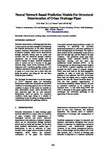
Figure years. Figure 6. 6. The The tendency tendency prediction prediction of of human human Echinococcosis Echinococcosis cases cases over over aa period period of of 60 60 years.

Figure 6 shows that the number of human Echinococcosis cases will increase steadily in 26 or 27 Figure 6 shows that the number of human Echinococcosis cases will increase steadily in 26 or 27 years, years, then reach a peak (about 1250) in 2039, before beginning to slowly decline, and finally then reach a peak (about 1250) in 2039, before beginning to slowly decline, and finally disappear. disappear.

3.2.2. Sensitivity Analysis 3.2.2. Sensitivity Analysis To create better control strategies for Echinococcosis infections, we would like to see what To create strategies for Echinococcosis infections, wemethods would like to see what parameters canbetter reducecontrol the basic reproduction number R0 . Based on the of reference [34], R parameters cana reduce the analysis basic reproduction number the methods reference [34], we performed sensitivity of several model parameters andonprovided someof useful strategies 0 . Based for performed controlling athe transmission of Echinococcosis. we sensitivity analysis of several model parameters and provided some useful strategies For the sensitivity analysis, we used Latin hypercube sampling (LHS) and partial rank correlation for controlling the transmission of Echinococcosis. coefficients to examine parameters which had a significant influence the basic For the(PRCC) sensitivity analysis, we used Latin hypercube sampling (LHS) and on partial rank production correlation number R0 . (PRCC) We chose sampleparameters size n = 3000, andhad the significance α = 0.05. Thebasic larger the PRCC coefficients tothe examine which a significantlevel influence on the production is in absolute value, the more important the parameters are for responding to the change of R 0 . A plus number R0 . We chose the sample size n = 3000, and the significance level  = 0.05. The larger the sign or minus sign means that the influence is positive or negative, respectively. The ordering of these PRCC is in absolute value, the more important the parameters are for responding to the change of PRCCs corresponds to the level of statistical influence that the parameter has on the variability of the R0 . Aproduction plus sign number or minusR sign means that the influence is positive or negative, respectively. The basic 0 . The PRCC values of six parameters are listed in Table 3 and are shown ordering in Figure of 7. these PRCCs corresponds to the level of statistical influence that the parameter has on the Table 3. Partial rank correlation coefficients (PRCCs) for the aggregate R0 and each input parameter variable.

Input Parameter A1 A2 β1 β2 σ α

The Basic Production Number R0 PRCC

p Value

0.0833 0.0148 0.8916 0.9530 −0.8307 0.0071

0.0000 0.4183 0.0000 0.0000 0.0000 0.6964

From Table 3 and Figure 7, we can confirm that parameters A1 , β 1 , and β 2 have a positive impact upon R0 , and that σ has a negative impact. We also know that R0 is not sensitive to parameters A2 and α. Further, Table 3 shows that the low parasite egg-to-livestock transmission rate β 2 (|PRCC| = 0.9530) has the greatest impact on R0 , followed by the livestock to dog transmission rate β 1 (|PRCC| = 0.8916), and then the high rate moving from infected to non-infected dogs σ (|PRCC| = −0.8307). Hence, from sensitivity and mathematical analysis, we conclude that the most effective approach for reducing the Echinococcosis infection is to decrease the parameters β 1 , and β 2 , and to increase the parameter σ.

1

A2 1 2 262 Int. J. Environ. Res. Public Health 2017, 14,  1

0.0148

0.4183

0.8916

0.0000

0.9530

0.0000

−0.8307 0.0071

0.0000 0.6964

*

12 of 14

*

0.8 0.6

PRCC

0.4 0.2

*

0 -0.2 -0.4 -0.6 -0.8

*

-1 A1

A2



1



2





coefficients (PRCC) results for the of R0 onofeach R0parameter. Figure 7. 7. Partial Partialrank rankcorrelation correlation coefficients (PRCC) results fordependence the dependence on each *parameter. denotes the value of PRCC is not zero significantly, where the significance level is 0.05. * denotes the value of PRCC is not zero significantly, where the significance level

is 0.05. From the above sensitivity analysis, to control Echinococcosis, some alternative strategies can be considered: should be 7, barred from slaughter and should fed uncooked offal, From Tabledogs 3 and Figure we can confirm that houses parameters andbe  A1 , 1 ,not 2 have a positive infection carcasses and offal should be burned or buried, the frequency of dog anthelmintic should be impact upon R0 , and that  has a negative impact. We also know that R0 is not sensitive to increased, the method of transmission and instructions in personal sanitation should be informed to parameters and Table 3 shows thatshould the low transmission A2 the  . Further, the public, and annual crop of newborn puppies beparasite reduced,egg-to-livestock etc. [1]. rate  2 (|PRCC| = 0.9530) has the greatest impact on R0 , followed by the livestock to dog 4. Conclusions transmission rate 1 (|PRCC| = 0.8916), and then the high rate moving from infected to nonEchinococcosis is of significant medical and economic importance in the Xinjiang Uygur infected dogs  (|PRCC| = −0.8307). Hence, from sensitivity and mathematical analysis, we Autonomous Region of China. It is one of the most important zoonotic diseases and it is of great conclude that the most effective approach for reducing the Echinococcosis infection is to decrease the social importance. This research investigates the modified grey model and the dynamic epidemic parameters 1 , and  2 , and to increase the parameter  . model for predicting the human Echinococcosis cases. In this study, the traditional GM(1,1) model, From thecorrection-based above sensitivitygrey analysis, to control Echinococcosis, some alternative strategies can be two residual models (PECGM(1,1), FGM(1,1)), and a multiplicative seasonal considered: dogs should be barred from slaughter houses and should not be fed uncooked offal, model ARIMA(1,0,1)(1,1,0)4 are applied, to analyze the surveillance data of Echinococcosis cases for infection carcasses and offal should be burned or buried, the frequency of dog anthelmintic should a short-term prediction comparison. Furthermore, a dynamic epidemic model for long-term prediction be increased, the method of transmission and instructions in personal sanitation should be informed is also established. to theThe public, and the annual crop models of newborn should is beable reduced, etc.an [1].accurate prediction fitting results of the grey showpuppies that FGM(1,1) to make for the Echinococcosis prevalence trend in Xinjiang. The results also demonstrate that there are obvious 4. Conclusions seasonal and periodic features in Echinococcosis cases in Xinjiang. Infection with Echinococcus remains Echinococcosis of significant medical and economic in theEfforts Xinjiang Uygur a major public healthisissue and the cases will continue to rise importance in the short-term. should be Autonomous of China. is one of most important zoonotic diseases andawareness. it is of great continued, forRegion both animals and Ithumans, bythe increasing training campaigns and public A dynamic epidemic prediction model can predict the future tendency very well. Its results demonstrate that, using current control options, human Echinococcosis cases will decrease around the 104th quarter. The basic reproduction number R0 = 0.541 indicates that, with the current control measures, human Echinococcosis cases will cease to exist in Xinjiang in the long run. To control human Echinococcosis, we could choose prevention and control strategies from decresae parameters A1 (annual crop of newborn puppies), β 1 (livestock to dog transmission rate), β 2 (parasite egg-to-livestock transmission rate), and increase the parameter σ (rate moving from infected to non-infected dog). However, elimination is a difficult goal to achieve, principally due to the disease transmission restriction and the control measures being implemented. It should be noted that the government and officials in Xinjiang have enlarged the propaganda and education on Echinococcosis control. There are many clear technological improvements in the diagnosis and treatment of human and animal Echinococcosis vaccinations against Echinococcus granulosus in animals. These new measures and technologies increase the efficiency of Echinococcus control programmes, potentially reducing the time required for its elimination. We hope that our work


13 of 14

may help in understanding the epidemic spreading phenomena and designing appropriate strategies to control Echinococcus infections in Xinjiang. Supplementary Materials: The following are available online at http://www.mdpi.com/1660-4601/14/3/262/s1. 1. Original GM(1,1) Model; 2. Grey-Periodic Extensional Combinatorial Model (PECGM(1,1)); 3. Modified Grey Model Using Fourier Series (FGM(1,1)). Acknowledgments: This research was supported by the National Natural Science Foundation of China (11401512, 11461073) and the Academic Discipline Project of Xinjiang Medical University-Health Measurements and Health Economics (XYDXK50780308). Author Contributions: Liping Zhang, Li Wang and Yanling Zheng analyzed the data; Xueliang Zhang and Yujian Zheng contributed materials; Liping Zhang and Kai Wang wrote the paper. Conflicts of Interest: The authors declare no conflict of interest.

References 1.

2. 3.

4. 5.

6. 7.

8. 9. 10. 11. 12. 13. 14. 15. 16.

Wang, K.; Zhang, X.; Jin, Z.; Ma, H.; Teng, Z.; Wang, L. Modeling and analysis of the transmission of Echinococcosis with application to Xinjiang Uygur Autonomous Region of China. J. Theor. Biol. 2013, 333, 78–90. [CrossRef] [PubMed] Budke, C.M.; Deplazes, P.; Torgerson, P.R. Global socioeconomic impact of cystic Echinococcosis. Emerg. Infect. Dis. 2006, 12, 296–303. [CrossRef] [PubMed] Craig, P.S.; McManus, D.P.; Lightowlers, M.W.; Chabalgoity, J.A.; Garcia, H.H.; Gavidia, C.M.; Gilman, R.H.; Gonzalez, A.E.; Lorca, M.; Naquira, C.; et al. Prevention and control of cystic echinococcosis. Lancet Infect. Dis. 2007, 7, 385–394. [CrossRef] Eckert, J.; Deplazes, P. Biological, epidemiological, and clinical aspects of echinococcosis, a zoonosis of increasing concern. Clin. Microbiol. Rev. 2004, 17, 107–135. [CrossRef] [PubMed] Eckert, J.; Deplazes, P.; Craig, P.; Gemmell, M.A.; Gottstein, B.; Heath, D.; Lightowlers, M. Echinococcosis in animals: Clinical aspects, diagnosis and treatment. In WHO/OIE Manual on Echinococcosis in Humans and Animals: A Public Health Problem of Global Concern, 1st ed.; Eckert, J., Gemmell, M.A., Meslin, F.X., Pawłowski, Z.S., Eds.; World Organisation for Animal Health (Office International des Epizooties) and World Health Organization: Paris, France, 2001; pp. 73–99. Moro, P.; Schantz, P.M. Echinococcosis: A review. J. Infect. Dis. 2009, 13, 125–133. [CrossRef] [PubMed] Pawlowski, Z.S.; Eckert, J.; Vuitton, D.A.; Ammann, R.W.; Kern, P.; Craig, P.S.; Grimm, F. Echinococcosis in humans: Clinical aspects, diagnosis and treatment. In WHO/OIE Manual on Echinococcosis in Humans and Animals: A Public Health Problem of Global Concern, 1st ed.; Eckert, J., Gemmell, M.A., Meslin, F.X., Pawłowski, Z.S., Eds.; World Organisation for Animal Health (Office International des Epizooties) and World Health Organization: Paris, France, 2001; pp. 20–71. Box, G.E.; Jenkins, G.M.; Reinsel, G.C.; Ljung, G.M. Time Series Analysis: Forecasting and Control, 4th ed.; John Wiley & Sons, Inc.: Hoboken, NJ, USA, 2015; pp. 1–727. Deng, J. Control problems of grey systems. Syst. Control Lett. 1982, 1, 288–294. Yin, M.S. Fifteen years of grey system theory research: A historical review and bibliometric analysis. Expert Syst. Appl. 2013, 40, 2767–2775. [CrossRef] Lin, C.S.; Liou, F.M.; Huang, C.P. Grey forecasting model for CO2 emissions: A Taiwan study. Appl. Energy 2011, 88, 3816–3820. [CrossRef] Lei, M.; Feng, Z. A proposed grey model for short-term electricity price forecasting in competitive power markets. Int. J. Electr. Power 2012, 43, 531–538. [CrossRef] Peng, Y.; Dong, M. A hybrid approach of HMM and grey model for age-dependent health prediction of engineering assets. Expert Syst. Appl. 2011, 38, 12946–12953. [CrossRef] Huang, K.Y.; Jane, C.J. A hybrid model for stock market forecasting and portfolio selection based on ARX, grey system and RS theories. Expert Syst. Appl. 2009, 36, 5387–5392. [CrossRef] Ma, Z.; Zhou, Y.; Wu, J. Modeling and Dynamics of Infectious Diseases, 1st ed.; World Scientific Publishing Company: Singapore, 2009; pp. 1–341. Cui, J.; Liu, S.F.; Zeng, B.; Xie, N.M. A novel grey forecasting model and its optimization. Appl. Math. Model. 2013, 37, 4399–4406. [CrossRef]


17. 18. 19. 20. 21. 22. 23. 24. 25. 26. 27. 28. 29.

30.

31. 32. 33. 34.

14 of 14

Hsu, C.C.; Chen, C.Y. Applications of improved grey prediction model for power demand forecasting. Energy Convers. Manag. 2003, 44, 2241–2249. [CrossRef] Lin, Y.H.; Lee, P.C.; Chang, T.P. Adaptive and high-precision grey forecasting model. Expert Syst. Appl. 2009, 36, 9658–9662. [CrossRef] Xie, N.M.; Liu, S.F. Discrete grey forecasting model and its optimization. Appl. Math. Model. 2009, 33, 1173–1186. [CrossRef] Chen, C.I.; Huang, S.J. The necessary and sufficient condition for GM(1,1) grey prediction model. Appl. Math. Comput. 2013, 219, 6152–6162. [CrossRef] Kumar, U.; Jain, V.K. Time series models (Grey-Markov, Grey Model with rolling mechanism and singular spectrum analysis) to forecast energy consumption in India. Energy 2010, 35, 1709–1716. [CrossRef] Lee, Y.S.; Tong, L.I. Forecasting nonlinear time series of energy consumption using a hybrid dynamic model. Appl. Energy 2012, 94, 251–256. [CrossRef] Tien, T.L. The deterministic grey dynamic model with convolution integral DGDMC(1,n). Appl. Math. Model. 2009, 33, 3498–3510. [CrossRef] Tseng, F.M.; Yu, H.C.; Tzeng, G.H. Applied hybrid grey model to forecast seasonal time series. Technol. Forecast. Soc. 2001, 67, 291–302. [CrossRef] Wang, Y.F. Predicting stock price using fuzzy grey prediction system. Expert Syst. Appl. 2002, 22, 33–38. [CrossRef] Zhou, Z.J.; Hu, C.H. An effective hybrid approach based on grey and ARMA for forecasting gyro drift. Chaos Soliton Fract. 2008, 35, 525–529. [CrossRef] Yao, A.W.; Chi, S.C.; Chen, C.K. Development of an integrated Grey–fuzzy-based electricity management system for enterprises. Energy 2005, 30, 2759–2771. [CrossRef] Kayacan, E.; Ulutas, B.; Kaynak, O. Grey system theory-based models in time series prediction. Expert Syst. Appl. 2010, 37, 1784–1789. [CrossRef] Yang, L.; Bi, Z.W.; Kou, Z.Q.; Li, X.J.; Zhang, M.; Wang, M.; Zhang, L.Y.; Zhao, Z.T. Time-series analysis on human brucellosis during 2004–2013 in Shandong province, China. Zoonoses Public Health 2015, 62, 228–235. [CrossRef] [PubMed] Chadsuthi, S.; Modchang, C.; Lenbury, Y.; Iamsirithaworn, S.; Triampo, W. Modeling seasonal leptospirosis transmission and its association with rainfall and temperature in Thailand using time-series and ARIMAX analyses. Asian Pac. J. Trop. Med. 2012, 5, 539–546. [CrossRef] Wang, T.; Liu, J.; Zhou, Y.; Cui, F.; Huang, Z.; Wang, L.; Zhai, S. Prevalence of hemorrhagic fever with renal syndrome in Yiyuan county, China, 2005–2014. BMC Infect. Dis. 2016, 16, 69. [CrossRef] [PubMed] Zhang, X.; Zhang, T.; Pei, J.; Liu, Y.; Li, X.; Medrano-Gracia, P. Time series modelling of syphilis in China from 2005 to 2012. PLoS ONE 2016, 11, e0149401. [CrossRef] [PubMed] Chinese Bureau of National Statistics. China Statistical Yearbook 2015, 1st ed.; National Bureau of Statistics of China: Beijing, China, 2015. Zhang, T.; Wang, K.; Zhang, X. Modeling and analyzing the transmission dynamics of HBV epidemic in Xinjiang, China. PLoS ONE 2015, 10, e0138765. [CrossRef] [PubMed] © 2017 by the authors. Licensee MDPI, Basel, Switzerland. This article is an open access article distributed under the terms and conditions of the Creative Commons Attribution (CC BY) license (http://creativecommons.org/licenses/by/4.0/).