Time Series Join on Subsequence Correlation - Semantic Scholar

Time Series Join on Subsequence Correlation Abdullah Mueen Department of Computer Science University of New Mexico [email protected]

Hossein Hamooni Department of Computer Science University of New Mexico [email protected]

Trilce Estrada Department of Computer Science University of New Mexico [email protected]

4

Abstract— We consider the problem of joining two long time series based on their most correlated segments. Two time series can be joined at any locations and for arbitrary length. Such join locations and length provide useful knowledge about the synchrony of the two time series and have applications in many domains including environmental monitoring, patient monitoring and power monitoring. However, join on correlation is a computationally expensive task, specially when the time series are large. The naive algorithm requires O(n4 ) computation where n is the length of the time series. We propose an algorithm, named Jocor, that uses two algorithmic techniques to tackle the complexity. First, the algorithm reuses the computation by caching sufficient statistics and second, the algorithm prunes unnecessary correlation computation by admissible heuristics. The algorithm runs orders of magnitude faster than the naive algorithm and enables us to join long time series as well as many small time series. We propose a variant of Jocor for fast approximation and an extension to a GPU-based parallel method to bring down the running-time to interactive level for analytics applications. We show three independent uses of time series join on correlation which are made possible by our algorithm.

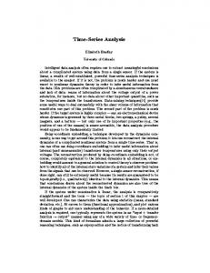
I. I NTRODUCTION Joining two time series in their most correlated segments of arbitrary lag and duration provides useful information about the synchrony of the time series. For example, Figure 1 shows exchange rates of two currencies, INR (Indian Rupee) and SGD (Singapore Dollar), against USD since 1996. The two time series have a mild negative correlation value when looked at globally. In Figure 1, the join segments are highlighted and they have a correlation coefficient of 0.94. The joined segments have a small lag and a duration of more than 3 years until 2007. This correlated segment suggests a strong similarity in the baskets of currencies to which INR and SGD were pegged to [6]. Note that, in general, the information of the peg-basket of a currency is confidential. The two currencies became uncorrelated after the join segment which denotes a major change in one of the currencies’ pegging and it is believed SGD stopped following USD and was pegged against a basket of other currencies mostly dominated by EUR in that time while INR kept following USD. Consider another example to motivate time series join on correlation. Normally, we expect respiration and systolic blood pressure to be uncorrelated for a healthy person. However, if we observe them becoming correlated, it is highly predictive of cardiac tamponade, an acute type of pericardial effusion in which fluid accumulates in the pericardium (the sac in which the heart is enclosed). Tamponade almost always results in

3

113 days

Indian Rupee (INR) Singapore Dollar (SGD)

2

1

0

-1

-2

-3

-4 3/27/1996

2/24/1998

1/25/2000

12/25/2001 11/25/2003 10/25/2005 9/25/2007

8/25/2009

7/26/2011

6/26/2013

Fig. 1. Two time series of currency exchange rates are joined to reveal high correlation in the past. The x-axis shows business days. The y-axis shows conversion rates of INR and SGD against USD after normalization.

death, unless quickly treated by pericardiocentesis, a procedure where fluid is aspirated from the pericardium. We can monitor the respiration and blood pressure for such correlations, that can exist in varying lag and duration depending on patients, to save lives. There are several possible ways two time series can be joined. The most obvious way is to join on overlapping timestamps, however timestamps are not always available and such joining assumes zero lag. If we use the content of the time series, we can join on highly correlated subsequences of the two time series. Most existing works on similarity join either consider fixed duration join or use some domain specific similarity function. We focus on joining two long time series or two sets of time series based on the most correlated (i.e. highest Pearson’s correlation coefficient) segments of arbitrary lag/locations and duration. Although we are using the term “join,” unlike relational joins, we are not merging or concatenating the participating time series when joining on correlation. Joining on correlation is very expensive computationally. The trivial algorithm to join two time series takes O(n4 ) time where n is the length of the time series. A computational time of this magnitude is unacceptable for a time-critical application as above and for many other time series datasets of moderate size. For example, the join operation shown in Figure 1 took 5 hours by the naive algorithm implemented in C++ on a third generation intel CPU. In this paper, we show a very fast algorithm, named Jocor (JOin on CORrelation), to join two time series on correlation that runs orders of magnitude faster than the naive algorithm while producing identical results. We extend Jocor in several directions. We show a faster approximate version that can produce approximate results within bounded accuracy. We propose using length-adjusted

correlation for time series join that can work better than Pearson’s correlation. We implement a parallel system in a GPU (Graphics Processing Unit) to reach interactive running time for large real-world datasets. We show two case studies in oceanography and power management where join segments are meaningful and can potentially be exploited to build applications. The paper is organized as follows. We describe the problem formally with necessary notation and background in Section 2. In Section 3, we describe the motivation of join on correlation with respect to existing algorithms. Section 4 discusses related work. Section 5 describes the algorithm with necessary theoretical development. In Section 6, we show the extensions of Jocor. Experimental results are shown in Section 7 and the case studies are shown in Section 8. II. P ROBLEM D EFINITION In this section, we define the problem and other notations used in the paper. Definition 1: A Time Series t is a sequence of real numbers t1 , t2 , . . . , tn where n is the length of the time series. A time series subsequence t[i : i + m − 1] = ti , ti+1 , . . . , ti+m−1 is a continuous subsequence of t starting at position i and length m. We would like to join two time series x and y of length n and m respectively. We assume n > m without losing generality. We define the time series join problem as below. Problem 1 (MaxCorrelation Join): Find the most correlated subsequences of x and y with length len ≥ minLength. We extend the definition to find α-approximate join. Problem 2 (α-Approximate Join): Find the subsequences of x and y with length len ≥ minLength such that the correlation between the subsequences is within α of the most correlated segments. In the above problems, we refer to maximizing the Pearson’s correlation coefficient when finding the most correlated subsequences. Pearson’s correlation coefficient is defined in equation 1. C(x, y) =

E[(x − µx )(y − µy )] σx σy

(1)

The person’s correlation is a good similarity measure because it can be computed by just a linear scan and it is scale and offset invariant. However, correlation coefficient is not a metric and it’s range is [-1,1]. If we just focus on maximizing positive correlations and ignore the negatively correlated subsequences, we can use z-normalized Euclidean distance and exploit the triangular inequality for efficiency. Z-normalized Euclidean distance is defined as below. If we are given two time series x and y of the same length m, we can use the euclidean norm of their difference (i.e. x-y) as the distance function. To achieve scale and offset invariance, we normalize the individual time series using z-normalization before the actual distance is computed. The z-normalized Euclidean distance is then computed by the formula

v um uX dist(x, y) = t (ˆ xi − yˆi )2

(2)

i=1

where x ˆi = σ1x (xi − µx ) and yˆi = σ1y (yi − µy ). The relationship between positive correlation and z-normalized Euclidean distance is the following [18]. dist2 (x, y) (3) 2m According to equation 3, maximizing correlation can be replaced by minimizing the z-normalized Euclidean distance. However, computing correlation coefficient or z-normalized Euclidean distance in the above formulation requires two passes (first, to compute µ and σ and second, to compute the distance). In contrast, we can compute the normalized Euclidean distance between x and y using five numbers derived from x and y. These numbers denoted statistics P areP P as2 sufficient P P x, y, x , y 2 and xy. in [22]. The numbers are The correlation coefficient can be computed as below. P xy − mµx µy (4) C(x, y) = mσx σy C(x, y) = 1 −

dist(x, y) =

p

2m(1 − C(x, y))

(5)

Computing the distance in this manner not only takes one pass but also enables us to reuse computations and reduce the amortized time complexity from linear to constant. Note that, the sample mean and standard can bePcomputed P deviation 1 1 from these statistics as µx = m x and σx2 = m x2 − µ2x , respectively. In this paper, we use the above formulation to compute correlation and/or z-normalized Euclidean distance. As used in [25][13], we normalize Euclidean distance based on length and we name it Length-adjusted z-normalized Euclidean distance (LA dist). dist(x, y) (6) m LA dist is not a metric but has one desirable property for join applications. It removes the bias of the correlation measure for shorter sequences. We defer the details of the discussion on bias until Section 6. LA dist(x, y) =

III. M OTIVATION In this section, we provide an analysis on different join possibilities for time series and motivate the necessity of joining time series based on highly correlated subsequences. In Figure 2 we show two time series x and y of equal length. They are the same currency exchange rates from Figure 1. When considering to join x and y, we have several options. First, we can measure the correlation or any other similarity measure between x and y globally and join them if the global correlation is above a certain threshold τ . Second, we can measure the cross-correlations between x and y for all lags and decide if any lagged correlation is larger that τ . Third, we

can measure the correlation between any pairs of subsequences of any length and decide if any of the pairs is larger than τ . And finally, we can find the most correlated join segments having a minimum length. In Figure 2, we show the matched segments for each of the four cases and the corresponding correlation values found in each case. Clearly, global correlation or cross-correlation do not produce good join segments. We achieve a very good join with τ = 0.95 as shown in Figure 2(C ). However, the join segment could be much larger if we set a required minimum length as shown in Figure 2(D). Note that, the correlation is smaller in this case than the best. Computing global correlation requires one linear scan and thus, it is O(n). Computing cross-correlation requires O(n log n) time using FFT algorithm. Computing correlation for arbitrary subsequences by a naive method requires O(n4 ) time which can reduce to O(n3 ) if we reuse computation by caching in the memory. For large data, such a large time complexity is unacceptable. To give an example, for n = 40, 000, the naive algorithm takes 11 days to finish. IV. R ELATED W ORK Existing work on time series join or data stream join can be classified into several categories. The first category joins on timestamps which is completely different from the problem we consider in this paper as there is no similarity comparison [9][23]. The second category of methods join time series based on Euclidean distance or Dynamic Time Warping (DTW) without any normalization to remove the scale and offset [8][24]. Thus, joining based on correlation cannot just work with these algorithms as correlation computation needs normalization for every subsequence. The third category of join methods are scale and offset invariant but unfortunately are not exact [11][12][10] and have no bound on the error. These methods propose unique ways of segmenting the time series for efficiency and find joining segments based on a similarity function over a feature-set. These methods usually have quite a few parameters to tune by the domain experts. In contrast, Jocor finds join segments with maximum correlation coefficient and requires only one domain-independent parameter, the minimum length of the segment which can be zero trivially. We also provide a fast approximation method which has tight error bound for confidence. We have the assumption that the joining series are uniformly sampled series i.e. the samples are taken at equal intervals and the intervals are the same for both the time series. Typical datasets adhere to this assumption and therefore, methods assuming equal sampling intervals are very common in the literature. Other than joining two time series, there is a rich literature of computing pairwise correlation values for a large number of evolving time series over fixed length sliding window [26], possibly with limited lags [22]. We fundamentally differ from them as we consider only archived time series for arbitrary lag and duration.

Algorithm 1 Join(x, y) Ensure: Return the locations and length of the most correlated segments of x and y 1: x ← (x-mean(x))/stdv(x) 2: y ← (y-mean(y))/stdv(y) 3: n ← length(x), m ← length(y) 4: best ← 0 5: for i ← 1 to m − minLength + 1 do 6: for j ← 1 to n − minLength + 1 do 7: maxLength ← min(m − i + 1, n − j + 1) 8: for len ← minLength to maxLength do 9: c ←Correlation(x[j:j+len-1],y[i:i+len-1]) 10: if c > best then 11: best ← c

A recent parallel work [10] on finding longest correlated subsequence between a query and a long time series has been published. In [10], authors propose an index structure and an α-skip method to find the longest match of a given query with correlation more than a threshold. There are some fundamental differences between [10] and our proposed work. Our work builds upon a bound on correlation measure across length described in [15] while [10] uses early abandoning technique based on the input threshold. Therefore, the speedup in [10] depends on the input threshold while our algorithm does not vary on the minimum length input. For a trivial input of zero, the method in [10] degenerates to brute-force search, while ours still finds the most correlated segment very quickly. In addition, we consider joining two large time series while [10] assumes the query be negligible in size. V. J OIN ON C ORRELATION We describe our algorithm in this section in two phases. We first show how to reuse the sufficient statistics for overlapping correlation computation and then show how to prune segmentpairs admissibly. We also provide pseudocode for clarity. We name our method Jocor (JOin on CORrelation) as mentioned before. The simplest algorithm to join two time series based on correlation is O(n4 ). Algorithm 1 shows such a method to find the most correlated join segments. The algorithm computes correlation of all the possible pairs of segments of all the lengths. Note that the correlation function in line 9 takes at least a linear scan over both the segments to compute the correlation. Algorithm 1 runs massive computation. For example, we have run a c++ implementation of this simple algorithm for the two time series in Figure 1 having four thousand observations each and it takes 5 hours to finish. We will use the Algorithm 1 as a skeleton and add statements around it to build Jocor. A. Overlapping Correlation Computation To reduce the massive computation required for algorithm 1, we need to use the overlap between segments while computing correlation. In this section, we show a method to cache

(A)  

(B)  

Correla'on:  -­‐0.1117  

3

3

(C)  

Correla'on:  0.8347  

4

2

2

1

1

0 0

Correla'on:  0.9599  

(D)   4

3

3

2

2

1

1

0

0

-1

-1

Correla'on:  0.9489  

-1 -1

-2

-2 -3 3/27/1996

-3

Full  Correla'on   1/25/2000

11/25/2003 9/25/2007

Fig. 2.

7/26/2011

-4

-2

-2

Cross-­‐Correla'on   3/27/1996 1/25/2000 9/25/2007

-3

𝜏  >  0.95  

-4 3/27/1996 1/25/2000 11/25/2003 9/25/2007 7/26/2011

minLength  >  7  years  

-3

-4 3/27/1996 1/25/2000 11/25/2003 9/25/2007 7/26/2011

The join segments and correlation coefficients for the same pair of currencies using different methods.

sufficient information to compute the correlation values at line 9 in constant time with O(n2 ) space. Let’s start with computing the shifted cross product between two time series. It can be done in O(n log n) time using the FFT algorithm as presented in lines 4 to 6 in the Algorithm 2. We are showing the steps in the Algorithm 2 without describing it elaborately. The steps produce an array that contains the sum of the products of the elements in x and y for different shifts of x. The output z of the Algorithm 2 is expressed more precisely as below. Here negative indices are assumed to return zeros. 0

zk =

m X

yl xk−m0 +l

(7)

l=1 0

Here m is the length of y and n0 > m0 is the length of x. Note that, zm is x.y and zk ’s for n0 + m0 ≥ k > m0 are sums of products of y with k-shifted x. Also note that the length of z is twice the length of x. We use the Algorithm 2 to fill in a two dimensional array that caches sufficient statistics to compute any correlation coefficient of any length at any locations of the two time series. Since the Algorithm 2 keeps one series fixed and shifts the other, we can shift the fixed series in an external loop to call the Algorithm 2 repeatedly to produce a set of z vectors. More precisely, we want to populate a set of cross products Z where Zi = multiply(x, y[i : m]). The cross products in Z are the most important statistics for any correlation computation between any segments. The dot product of two subsequences of x and y starting at j and i-th locations, respectively, with length len can be computed as follows. Zi [m − i + j] − Zi+len [m − i + j] Pm−i = l=1 yl+i xm−i+j−(m−i)+l Pm−i−len − l=1 y x Pm−i Pm−i l+i+len m−i+j−(m−i−len)+l = l=1 yl+i xj+l − l=len yl+i xj+l Plen = l=1 yl+i xj+l The complexity to compute the cache Z is O(n2 log n) which may seem to be high. However, having such a quadraticspace cache reduces the join algorithm from O(n4 ) to O(n3 ). Where in the Algorithm 1 do we use the above caching mechanism? The Algorithm 3 describes the complete Jocor method transformed from the Algorithm 1. Lines 4-5 compute

Algorithm 2 multiply(x, y) Ensure: Return the shifted dot products for x and y 1: n0 ← length(x), m0 ← length(y) 2: x← append(x, n0 -zeros) 3: y← append(reverse(y), (2n0 − m0 )-zeros) 4: X←FFT(x) 5: Y←FFT(y) 6: Z←X.Y 7: z←iFFT(Z)

the cache and line 12 uses the cache to retrieve the sum-ofproducts of the subsequences of x and y. Note the correlation computation in line 13 is a constant time operation assuming the mean and standard deviations are already known. We use cumulative sums to generate the means and standard deviations as described in [19] and in the definition section. The remaining parts of the Jocor algorithm will be explained in the next section. B. Pruning Uncorrelated Locations We describe our second technique to further optimize the Algorithm 1. We aim to build a mechanism to skip some of the lengths in the loop at line 8. We use a novel distance bound across lengths [15] to compute the step size dynamically instead of incrementing the len variable by one. If we know the distance between two subsequences of length len as d = dist(x[j : j + len − 1], y[i : i + len − 1]), the lower bound for the dnext = dist(x[j : j + len], y[i : i + len]) can be expressed as below. Here, z needs to be larger than any normalized value in the dataset and can be pre-computed. d2LB

len = ( (1+len) + 2 = fd

len 2 −1 2 d (1+len)2 z )

We want to use the above bound to find a safe stepSize that jumps over all the unnecessary lengths which would not have more correlation than the best correlation discovered so far. Note that, in the bound equation, the d2LB is a fraction 0 < f < 1 of d2 and the larger the len the more close the fraction is to one. A pessimistic choice would be to assume that we repeatedly apply the fraction for len instead of the fractions for len + 1, len + 2, . . . , len + S where S is a stepSize. For example, 0.64 < 0.6×0.7×0.8×0.9. Therefore, d2LB S = f S d2

Algorithm 3 Jocor(x, y) Ensure: Return the locations and length of the most correlated segments of x and y 1: x ← (x-mean(x))/stdv(x) 2: y ← (y-mean(y))/stdv(y) 3: n ← length(x), m ← length(y) 4: for i = 1 to m do 5: Zi ← multiply(x, y[i : m]) 6: best ← 0 7: for i ← 1 to m − minLength + 1 do 8: for j ← 1 to n − minLength + 1 do 9: maxLength ← min(m − i + 1, n − j + 1) 10: len ← minLength 11: while len ≤ maxLength do 12: sumXY ← Zi [m − i + j] − Zi+len [m − i + j] sumXY −µx µy 13: c← lenσx σy 14: if c > best then 15: best ← c len len 2 −1 + (1+len) 16: f ← ( (1+len) 2z ) 1−best 1 )c 17: stepSize ← blog 1−c ÷ (log f − len 18: if stepSize ≤ 0 or stepSize ≥ len then 19: stepSize ← 0 20: len ← len + stepSize + 1

and S is a safe stepSize if d2LB S ≥ d2best . Using the equality, we solve for S exploiting the Taylor series and ignoring the higher order terms. ⇒ ⇒ ⇒ ⇒

d2best S d2 = f (len+S)(1−Cbest ) = fS len(1−C) S best ) log(1 + len ) + log (1−C (1−C) = S log f (1−Cbest ) S len + log (1−C) = S log f (1−Cbest ) 1 ) S > log (1−C) ÷ (log f − len

In the Algorithm 3, we use the above equation to determine the stepSize for the innermost loop at line 17. The fraction f is computed at line 16. Note that we take floor of S and check the range of stepSize at line 18 so we don’t violate the S condition for taylor expansion which is len ≤ 1. Computing the maximum normalized value: As described in the previous section, z is the empirical maximum normalized value in the dataset over all possible means and variances at all lengths. There exists an algorithm to exactly compute the maximum value for z in O(n2 ) time (shown in [15]) for every length. To join time series on correlated subsequences, the O(n2 ) is acceptable as the entire algorithm has higher complexity. However we can set a pessimistic z value in linear time by normalizing the time series globally and taking the twice of the absolute value of any individual observation. Mathematically, by setting z = 2 ∗ max(abs(x), abs(y)). Unfortunately, there can be datasets where noisy spikes can massively impact the empirical value of z and thus reducing the benefit of the bounds. The value of z can be thought of as the largest possible value of an observation in the dataset if the

data is z-normalized prior to any processing. A z-normalized time series has mean and variance equal to 0 and 1 and the maximum value can be infinitely large. We can make probabilistic assumption about z when the time series are large and roughly normally distributed. If we assume that an unknown observation z will follow a standard normal we R C distribution, x2 can argue that, P (z > C) = 1 − √12π −∞ e− 2 dx. Thus, a value of 5 (i.e. 5σ away from the mean) has a very small probability (10−5 ) to appear in an unknown observation of a normalized time series. In this way, we can set a hard-coded value of 5 for z for noisy datasets and have high confidence that the bound is almost always correct. VI. E XTENSIONS Jocor is an exact method finding the most correlated segments. In this section, we present two extensions of the Jocor algorithm. A. Join on Length Adjusted Distance Our first extension is to join on length-adjusted znormalized Euclidean distance (LA dist) instead of the Pearson’s correlation coefficient. Although, in [16] and [25] authors have used such distance measure, we motivate the necessity of LA dist for time series join. We first experiment to see the distribution of the maximum correlation for different lengths. Figure 3 shows how the maximum correlation between all segment-pairs of a certain length decreases as we increase the length. In other words, the shorter subsequences tend to be more correlated than their extended subsequences. This creates a strong bias in Jocor so it produces the best matching segments of a length close to the minLength. The minLength is 100 for Figure 3. x1.5x10-­‐3   Correla6on   Length-­‐adjusted  z-­‐normalized  Euclidean  Distance  

2

1.5

2

Best  Correla6on  

1.5

1

1

0.5

0.5

Best  LA_dist

0 100

200

300

400

Lengths  

500

0 600

700

800

Fig. 3. For the pair of currencies shown in Figure 2, The best Pearson’s correlation coefficients and the best length-adjusted Euclidean distances are shown for various lengths. Pearson’s correlations decrease with increasing lengths. While the length-adjusted Euclidean distance can report a longer join segment with less Pearson’s correlation coefficient than the best one.

Being adjusted by the length, LA dist prefers a long sequence of a slightly less correlation over a short sequence of the highest correlation. As seen in this example, LA dist finds the best match at length more than 400 although the correlation for the match is not the best. It can be clearly seen in the Figure 3 that the best match found by LA dist is at a length where the correlation has started to decrease drastically. How do we change our Jocor algorithm to accommodate the optimization for LA dist? We need to compute the LA dist instead of the correlation, c, at line 13 using the equations 5

and 6. We also need to change the “if” condition to maximize LA dist at line 14. However, these are simple changes by definition. The step size at line 17 is derived for correlation and we need to find the proper step size for LA dist. We start with restating the definition of LA dist. qP y −µ 2 m xi −µx 1 − i σy y ) LA dist(x, y) = dist(x,y) = i=1 ( σx m m The lower bound for the LA dist can be computed from the lower bound of the z-normalized Euclidean distance found in the previous section. d2LB d2LB

⇒ (1+len)2 ⇒ LA dist2LB

len = f d2 = ( (1+len) +

len 2 −1 2 d (1+len)2 z )

2

len d = (1+len+z 2 ) len2 len 2 = (1+len+z 2 ) LA dist 2 0 = f LA dist

As step size for correlation is computed from the lower bound, we can compute the step size for the LA dist as below. In the derivation, we take the largest value for the log(1 − S len+S ) at the limit S → 0. ⇒ ⇒ ⇒ ⇒

LA d2best 0S LA d2 = f len(1−Cbest ) 0S (len+S)(1−C) = f S best ) 0 log(1 − (len+S) ) + log (1−C (1−C) = S log f 2 S S best ) 0 log (1−C (1−C) = S log f + (len+S) + 2(len+S)2 1 best ) 0 S > log (1−C (1−C) ÷ (log f + len )

+ ...

Thus, changing the lines 13-17 in the Jocor algorithm is sufficient to achieve a Jocor for LA dist.

length len. If we skip every k positions of the inner time series, the number of pairs of locations is reduced to (n − minLen+1) (m−minLen+1) . Assume the best location pair, o, k is one of the pairs that the algorithm misses that has a distance d. There exists a pair p that the algorithm compared and we can extend that pair at most k-steps to obtain the optimal pair. By definition, our approximate algorithm outputs either p or another pair that has less distance than the pair p. If we assume, pessimistically, p has the minimum possible distance (i.e. dk ) then the distance of o should be larger than the lower k bound for k-step extension of p. Therefore, d2 > d2k fminLen . Note the use of the trivial lower bound here. To demonstrate the above theorem in action, we do an experiment varying the skipSize k and running the Jocor algorithm to find the best computed pair. Note that, k = 1 gives the optimal distance. We plot the discovered best correlation in red and the worst case drop in the correlation that could be possible for a skipSize k in green. The discovered best correlation is mostly the same as the optimal one and it never drops below the green curve showing the theorem is correct for these six datasets. In the bottom four datasets the worst possible correlation is even more than 0.9. Therefore, we can easily set skipSize k to 32 and get 32× speed-up. However for the powerConsumption dataset we observe a massive error range that carries no information. The reason is the dataset has large spikes that cause a large z value and as a result, a very small bounding factor. Correla7on  

Correla7on  

B. Approximate Join

0

0.86

-0.4

0.84

-0.8

0.82

Our algorithm in the previous section is an exact algorithm that runs faster than the trivial counter part. For short signals, the exact method is the best choice and reasonably fast. However, for long time series which are of the order of 105 , we need a really fast approximation technique trading off some accuracy within a bound. In this section we describe how to convert the Jocor algorithm to an approximation algorithm within a bound. The technique is very simple. We skip every k positions of the inner time series in line 8 of the Jocor algorithm. The effect of such skipping is that we may miss the exact solution and find a very close approximate solution. We provide a bound on the worst-case-loss in correlation if we adopt the skipping technique for the inner time series. Note that, skipping every 8 positions in this way is not the same as 8-way downdamping before joining the time series because the correlation coefficients are still computed in the original resolution. Before we derive the error bound, let us first discuss the trivial bound for correlation across length. Recall, the boundlen len 2 −1 ing factor f for a length is ( (1+len) + (1+len) which 2z ) is a monotonically increasing function over length. If the user supplied minimum length is minLen then the trivial factor for minLen minLen 2 −1 any length is fminLen = ( (1+minLen) + (1+minLen) . 2z ) Now, if we don’t skip anything, i.e. k = 1, then we compare (n − len + 1)(m − len + 1) pairs of locations for one specific

PowerConsump7on  

0.8

BloodPressure  

-1.2 0.996

0.99

0.992

0.98

0.988

0.97 0.96

0.984 0.98

Currency  

0.95 1

EEG  

0.976 0.97

0.9995 0.999 0.9985 0.998 0.9975 0

Reported  

0.4

0.88

StarLightCurve   5

10

15

20

25

30

35

0.96 0.95 0.94 0.93 0.92 0.91

RandomWalk   0

5

10

Fig. 4.

15

20

25

30

35

skipSize  

skipSize  

Approximation bounds for different datasets.

To summarize, if one discovers a 0.2 correlated pair using skipSize 32, it is highly likely there exists no good pair. If one discovers 0.9 correlated pair, the pair is as good as the best one. An additional note, the speedup does not depend on which time series we place in the inner loop. But the space usage can be reduced by placing the longer time series in the inner loop. VII. E XPERIMENTS We have all of our code, data, slides, pdfs and additional experiments available on anonymous repository [1] and the access password is JOCOR2014. Our method is completely reproducible and easy to use for visualization. We provide a matlab script that can be used to produce all the join visualizations shown in this paper.

9

104 103

EEG RW Power LightCurve RatBP BF

102 101 100

EEG RW Power LightCurve RatBP

103

102

101

100

10-1 0

0.5

1

1.5

2

2.5

Time Series Length

3

3.5

4 x 104

0

10

20

30

40

50

60

70

skipSize (k)

Ratio of Execution Times

104

105

Execution Time (Seconds)

Execution Time (Seconds)

106

EEG RW Power LightCurve RatBP

8 7 6 5 4 3 2 1 0 0

0.5

1

1.5

2

2.5

3

Time Series Length

3.5

4 x 104

Fig. 5. Experimental demonstration of speedup of the three different algorithms. (left) A1 over Brute Force method. (middle) A2 for various skipSize. k = 1 denotes the runtime for A1 . (right) A3 over A1 .

We use six datasets for our experimentation. The datasets are mainly of two different forms. First, two long time series from two different sources. Second, many short time series from the same source. To use the second form of data, we divide the short series into two equal partitions and concatenate the short series in each partition to create two long time series. Performing join on these two time series is equivalent to performing join between the two partitions of time series except the overlapping segments created because of the concatenation. Each of the dataset has potential to grow to millions of time series and thus, a scalable algorithm for join computation is a necessity for them. •

• •

•

•

•

Power: 520K points long whole house power consumption sequence that captures important patterns on the individual appliances operating at an instance of time [14]. We join the whole house power consumption to that of the refrigerator. LightCurve : 8000 star light-curves are collected from [20]. Each light-curve has 1000 observations. EEG: EEG traces having roughly 180K observations from two electrodes of the same patient in the same recording [17]. Currency: Daily conversion rates of different currencies from USD since 1996 [3]. We have 190 currency conversion rate and we have up to 4000 observations per currency. BloodPressure: The blood pressure of Dahl salt-sensitive (SS) rat collected to study baroreflex dysfunction [7]. We have 100 blood-pressure sequences each having 2000 observations. Random Walk (RW): Synthetically generated random walks.

We have experimented with four different versions of our algorithm described in Algorithm 3. The algorithms are all implemented in C++ and the source code is available in the webpage. For the Algorithm 2, we use fftw3 library. • • •

•

Exact Join (A1 ): This is the Algorithm 3 which is guaranteed to find the most correlated subsequence. Approximate Join (A2 ): This is the algorithm which skips every k positions of the inner time series in Algorithm 3. Length-adjusted Join (A3 ): This algorithm optimizes the length-adjusted correlation instead of the Pearson’s correlation in the Algorithm 3. GPU-based Join (A4 ): The Algorithm 3 has been re-

designed to exploit the available GPU. A. Scalability Jocor is the first algorithm to suggest time series join on correlation. There are other techniques for online correlation mining, for example, BRAID [22] and StatStream [26]. Both of the methods consider the correlation of the most recent windows of the streams. Jocor is not an online algorithm and it joins offline data for all possible windows. Most of the proposed methods that can be converted to time series join methods are not exact, i.e. the algorithms can miss the best join segment. As discussed in the Applications section, the exactness is a very desirable property for time series join. Jocor is an exact algorithm to join time series and therefore, is computationally more expensive than other approximate correlation mining algorithms. To compare the speed of Jocor, we use the naive algorithm with a quadratic cache to store sufficient statistics. Thus, the naive algorithm has O(n3 ) time complexity. For simplicity, we always use equal sized time series (i.e. n = m) to join although our method is not limited to that. We vary n and measure the running time of Jocor and the naive brute force algorithm with equal memory footprint to show the speedup and goodness of the algorithm. Note that, Jocor has no parameter other than the minimum join length which can trivially be set to zero without sacrificing speed-up. In our experiments, we set minLength = 100 unless otherwise specified. Figure 5(left) shows the speed-up Jocor (A1 ) can achieve for different datasets over naive Brute Force. Note that, naive algorithm takes same time for all of the datasets. Jocor gets the smallest speed-up of roughly 2× for the Power dataset. The reason is the same as explained before in the Approximation section; the Power dataset has large spikes that corrupts the value of z which in turn reduces the pruning power of our method. We then test the speed-up Jocor can achieve by simple approximation algorithm (A2 ). We vary the skipSize (k) and measure the running time. Note that k = 1 is the same as the Jocor algorithm. As shown in Figure 5 (middle), there is a linear speed-up as we increase k. Note the log scale in the y-axis. For this experiment, we fix n = 8000. We test the speed-up of the Jocor algorithm when it optimizes for the length-adjusted Euclidean distance. We vary the time series length and measure the speed-up over the algorithm

A1 shown in Figure 5(right). There is no clear trend in the ratio of the running times of A3 over A1 as we increase lengths. As a general statement, we see that join on the length-adjusted Euclidean distance takes more time than that on the Pearson’s correlation and the exact ratio changes with the increase of length, as well as, with datasets. A reasonable question would be to understand the distribution of the time spent in parts of the algorithm. We report the breakdown of the running time for the two major parts of the Algorithm 3. The first six lines in Jocor compute the sufficient statistics while the remaining lines search the best correlated segment. In Figure 6(left), we show the time for the two disjoint parts. The statistics-computation takes insignificant amount of time compared to the exact search. However the gap between the two parts of the code is reduced if we use the approximation technique with a skipSize, k = 32 and becomes significant. B. Pruning Power The scalability experiments have demonstrated the speedup. However one may raise concern that the speed-up might have resulted from implementation differences. In this section we show the pruning power of our novel bounds. We define the pruning power as the average percentage of lengths that Jocor can skip in the third loop (line 11) in Algorithm 3. We measure the pruning power for different lengths of the joining time series of the datasets and show in Figure 6(middle). Most of the datasets achieve 0.98 or more pruning rate which means, on average, Jocor prunes 98% of the lengths for any location-pair (i, j). The rate increases as the joining sequences become larger. The Power dataset shows significantly low pruning rate because of reasons explained earlier. The pruning power of the method depends on the value of z. Large values of z give less pruning performance. We experimentally validate the statement in Figure 6(right). For small z values, the datasets achieve close to 100% pruning rate and, with the increase of z pruning rate decreases depending on the datasets. As usual, Power performs worse. Note that the larger values of z are less probable and we can achieve massive speed-up if we manually set a small z sacrificing the exactness guarantee. C. Scalability on GPU We also run a GPU-based implementation of our method on a commodity GPU. It is a GeForce GT 630M with 96 cores and 800 MHz graphics clock. There is a 1GB memory on the card. We use the maximum number of threads (i.e. 32x16=512) allowed and we use 256 (16x16) blocks, more than the number of cores in the GPU. We need to chunk the time series in segments so the memory of each core in GPU is just sufficient to perform join operation on a pair of chunks and the number of processes launched in the GPU is minimized. This chunking is done in the CPU after the sufficient statistics are computed at line 6 of Jocor. The algorithm sends every pair of chunks to the GPU’s global memory, one by one, to compute the best join segment.

The exact version of Jocor gains nothing when ported on GPU because of the thread synchronization i.e. each thread runs different number of the main loop and all threads should wait for the slowest one to finish. In Figure 7(left) we show the speed-up of the exact version where the ratio remains very close to one or sometimes less than one. One interesting observation is the speed-up for the Power data. Recall, Jocor performs worse on the Power data because of lack of variance in the number of iterations of the “while” loop. This makes the Power data a perfect fit for speed-up by parallelization as all the threads are running roughly the same amount of times with a balanced load. Next, we test the speed-up for z = 3 and show the results in Figure 7(middle). We have around 2× to 6× speed-up from the single CPU version. We do not consider it a success as we have 96 cores in the GPU. Finally, we test the speed-up for z = 3 and k = 32 and show the results in Figure 7(right). Here we achieve up-to 47× speed-up which close to 50% of the number of cores. Although the above speedup is promising, the question remains if this is sufficient for interactive applications. Of course, the answer depends on the data size. The absolute running times of the GPU implementation with z = 3 and k = 32 for a join of size 10,000x10,0000 are all smaller than 10 seconds. It is a good enough size for joining tables of time series such as our LightCurve and RatBP datasets and many other datasets in the UCR time series archive [4]. VIII. A PPLICATIONS In this section, we show three scenarios of data mining that can use time series join on correlation. A. Join Based Similarity Search Time series join on correlated subsequence can be applied in higher level analytics. Imagine that we have a large time series of power consumption of a household refrigerator [14] shown in Figure 8(top). The data has more than 500 thousands observations in each of the time series. As an analyst, one can browse the time series with a small viewing window and arrive at the Figure 8(middle). The power consumption of a refrigerator has a specific cyclic pattern with on-off segments. The ON-OFF segments can be of different length and the Figure 8(middle) has several long ON segments sequentially. The analyst can select a region (shown in red) in the viewing window which includes the uncommon segment and queries for similar patterns in the entire time series. This action of flexibly selecting (maybe using a mouse) the query is a powerful tool for analysis tasks and creates a havoc for traditional similarity search methods. Traditional methods compare the entire query using various similarity measures such as correlation, Euclidean distance, Dynamic Time Warping (DTW) etc. and finds the best match. However traditional methods can not ignore flexible ends which is a requirement from analysts who are unsure about the exact query length. The Figure 8(bottom) shows the best join segment for the selected query where the two long cycles and the high cycle

Statistics Exact, k=1 Approximate, k=32

1

Rate of Pruning

104 103 102 101

1

0.98

0.98

0.96

0.96

0.94 0.92 0.9

EEG RW Power LightCurve RatBP

0.88 0.86

100

0.84

10-1

0.8

0.82

0

0.5

1

1.5

2

2.5

3

Time Series Length

3.5

Rate of Pruning

Execution Times (Seconds)

105

0.94 0.92

EEG

0.9

RW

0.88 0.86

Power LightCurve

0.84

RatBP

0.82

4 x 104

0

0.5

1

1.5

2

2.5

3

Time Series Length

3.5

2

4 x 104

4

6

8

10

z

12

14

16

18

20

EEG RW Power LightCurve RatBP

45 40 35 30 25 20 15 10 5 0

1000 2000 3000 4000 5000 6000 7000 8000 9000 10000

50

EEG RW Power LightCurve RatBP

45 40 35 30 25 20 15 10 5 0

1000 2000 3000 4000 5000 6000 7000 8000 9000 10000

Time Series Length

Time Series Length

Ratio of Execution Times (A1/A5)

50

Ratio of Execution Times (A1/A5)

Ratio of Execution Times (A1/A5)

Fig. 6. (left) Break down of the computation. The statistics computation time and the join computation time are separately shown. (middle) The rate of pruning achieved by our novel lower-bound. (right) Impact of z on the rate of pruning. 50

EEG RW Power LightCurve RatBP

45 40 35 30 25 20 15 10 5 0

1000 2000 3000 4000 5000 6000 7000 8000 9000 10000

Time Series Length

Fig. 7. The speed-up of a GPU-based implementation of Jocor over a CPU based implementation, A4 over A1 (left) when both implementation are exact. (middle) when both implementations are probabilistically accurate for z = 3. (right) when z = 3 and k = 32. All of the three plots have identical y-axis.

matched almost perfectly with a correlation value of 0.97. More importantly, the algorithm did not find any other match with correlation more than 0.95 which suggests the pattern is a rare one. We use traditional similarity search with 0.9 correlation threshold, we miss this great match and find some spurious matches. 1500

method. As show in the Figure 9, join based similarity can cluster better than DTW. The reason for join segments working better than the DTW alignment is that there are irrelevant phonemes segmented out from the adjacent words into our samples. Thus DTW suffers from aligning irrelevant phonemes to relevant ones while Jocor excludes those phonemes for the lack of good matches.

500 0

0.5

1

1.5

2

2.5

3

3.5

4

4.5

5

x105

600 500 400 300 200 100 0 5.14

5.141

5.142

5.143

5.144

5.145

5.146

5.147

5.148

5.149

5.15 x105

English

Arabic

Mandarin

Join Based Similarity

0

Dynamic Time Warping

1000

4 3 2 1 0 -1

1.897

1.8975

1.898

1.8985

1.899

1.8995

x105

Fig. 8. (top) A series of power consumption of a household refrigerator. (middle) An interesting subsequence selected as a query by an analyst. (bottom) The best join segments are shown. The query is shown in red and the match is shown in blue.

B. Join Based Clustering Join segments can represent the similarity between two time series which has already been used in [25][13]. We have done a small experiment to demonstrate the potential of such use. We have taken six audio samples where subjects say the name “Stella.” We have collected the data from the GMU speech accent archive [5] and our samples cover native english speakers, arabic accent and mandarin accent. We have taken envelops of the signals (shown in red in the Figure 9) and used both DTW and Jocor to measure the similarity among the signals and plotted dendrograms based on Ward’s linkage

Fig. 9. Dendrograms based on DTW and correlation coefficient of the join segment.

C. Join Based Filtering Time series join on correlation can provide interesting perspective on multivariate data. We perform a case study to demonstrate it. We have taken a dataset [2] of salinity and temperature of a circular region around station ALOHA (22◦ 450 N 158◦ W) in the pacific ocean shown in Figure 10. Ocean salinity has a yearly periodicity for the surface current and a daily periodicity for the tides. Ocean temperature is roughly constant except occasional drops (see Figure 10). Each time series has 1.8 million observations and note that they represent only one location of the earth. Performing a join on such long pair of time series is impossible by the naive algorithm which has been made possible by Jocor.

6 5 4

6

4

4

2

2

0

0

-2

3

-2

2

-4

1

-6

0

-8

-1

-10

11-Jan, 1999

-2

-4 -6 -8 -10

18-May, 2003

-12

07:01:11 08:24:31

09:47:51

11:11:11 12:34:30

Fig. 11.

13:57:50

-14

09:24:22

10:47:42

Celsius 2000

2001

2003

2004

2005

27 26 25 24 23 22

1998

12:11:02

2007

Salinity (PSU) 2000

2001

13:34:22

14:57:42

06:48:55

08:12:15

09:35:35

10:58:55

12:22:15

13:45:35

Three most correlated joins in three different days when temperature and salinity follow the same pattern.

36 35 34 33 32 31

1998

12-Oct, 2003

-12

-14

2003

2004

2005

2007

2008

Fig. 10. The thermosalinograph dataset. Temperature and salinity of station ALOHA for nine consecutive years.

Typically, the relationship between salinity and temperature depends on the density of the water and there can be many other factors that are important in their relationship [21]. We ask the question if there was any day in the past when the two variates were highly correlated denoting the fact that other variables were roughly constant. We have found three days in Figure 11 when the temperature and salinity of the area are highly correlated. Such correlated segments are evidences of “everything being right” in the system. In these three days, first, the ship that recorded the data operated in a very small area and had consistent noisefree measurements. Second, the water density was close to constant to observe the correlation. Third, the periodic change in temperature in Figure 11(middle) suggests a front of an eddy was passing the area. Thus time series join can point to the clean and noise-free part of the data that can be used to reason about many properties of the underlying system. IX. C ONCLUSION Time series join on subsequence correlation is a promising analysis tool that can potentially be used in many domains including environmental monitoring, power management and acoustic monitoring. In this paper we have described an efficient algorithm to perform join on subsequence correlation. The algorithm is orders of magnitude faster than the brute force solution while producing the same results. R EFERENCES [1] Anonymous code and data repository for the paper. https://files. secureserver.net/0fzoieonFsQcsM. [2] Hot data reports. http://www.soest.hawaii.edu/HOT_WOCE/ ftp.html. [3] Quandl - find, use and share numerical data. www.quandl.com. [4] The ucr time series classification/clustering homepage. www.cs.ucr. edu/˜eamonn/time_series_data/. [5] Weinberger, steven. (2014). speech accent archive. george mason university. http://accent.gmu.edu. [6] Wikipedia articles and references in there for SGD and INR. en.wikipedia.org/wiki/Singapore_dollar , en.wikipedia.org/wiki/Indian_rupee.

[7] S. M. Bugenhagen, A. W. Cowley., and D. A. Beard. Identifying physiological origins of baroreflex dysfunction in salt-sensitive hypertension in the dahl ss rat. Physiological Genomics, 42:23–41, 2010. [8] Y. Chen, G. Chen, K. Chen, and B.-C. Ooi. Efficient processing of warping time series join of motion capture data. In Data Engineering, 2009. ICDE ’09. IEEE 25th International Conference on, pages 1048– 1059, 2009. [9] A. Das, J. Gehrke, and M. Riedewald. Approximate join processing over data streams. In Proceedings of the 2003 ACM SIGMOD international conference on Management of data, SIGMOD ’03, pages 40–51, 2003. [10] Y. Li, L. H. U, M. L. Yiu, and Z. Gong. Discovering longestlasting correlation in sequence databases. In Proceedings of the VLDB Endowment, Vol. 6, No. 14, pages 1666–1677, 2013. [11] Y. Lin and M. McCool. Subseries join: A similarity-based time series match approach. In Advances in Knowledge Discovery and Data Mining, volume 6118, pages 238–245. 2010. [12] Y. Lin, M. D. McCool, and A. A. Ghorbani. Time series motif discovery and anomaly detection based on subseries join. In IAENG International Journal of Computer Science, volume 37(3). 2010. [13] J. Lines, L. M. Davis, J. Hills, and A. Bagnall. A shapelet transform for time series classification. In Proceedings of the 18th ACM SIGKDD International Conference on Knowledge Discovery and Data Mining, KDD, pages 289–297, 2012. [14] S. Makonin, F. Popowich, L. Bartram, B. Gill, and I. V. Bajic. AMPds: A Public Dataset for Load Disaggregation and Eco-Feedback Research. In Electrical Power and Energy Conference (EPEC), 2013 IEEE, pages 1–6, 2013. [15] A. Mueen. Enumeration of time series motifs of all lengths. ICDM, pages 547–556, 2013. [16] A. Mueen and E. J. Keogh. Logical-shapelets: An expressive primitive for time series classification. In KDD, pages 1154–1162, 2011. [17] A. Mueen, E. J. Keogh, Q. Zhu, S. Cash, and M. B. Westover. Exact discovery of time series motifs. In SDM, pages 473–484, 2009. [18] A. Mueen, S. Nath, and J. Liu. Fast approximate correlation for massive time-series data. In SIGMOD Conference, pages 171–182, 2010. [19] T. Rakthanmanon, B. Campana, A. Mueen, G. Batista, B. Westover, Q. Zhu, J. Zakaria, and E. Keogh. Searching and mining trillions of time series subsequences under dynamic time warping. KDD ’12, pages 262–270, 2012. [20] U. Rebbapragada, P. Protopapas, C. E. Brodley, and C. Alcock. Finding anomalous periodic time series. Mach. Learn., 74(3):281–313, 2009. [21] D. L. Rudnick and R. Ferrari. Compensation of horizontal temperature and salinity gradients in the ocean mixed layer. Science, 283(5401):526– 529, 1999. [22] Y. Sakurai, S. Papadimitriou, and C. Faloutsos. Braid: Stream mining through group lag correlations. In SIGMOD Conference, pages 599–610, 2005. [23] J. Xie and J. Yang. A survey of join processing in data streams. In Data Streams, volume 31 of Advances in Database Systems, pages 209–236. Springer US, 2007. [24] D. Yankov, E. Keogh, S. Lonardi, and A. W. Fu. Dot plots for time series analysis. IEEE 24th International Conference on Tools with Artificial Intelligence, pages 159–168, 2005. [25] L. Ye and E. Keogh. Time series shapelets: a new primitive for data mining. In Proceedings of the 15th ACM SIGKDD international conference on Knowledge discovery and data mining, KDD, pages 947– 956, 2009. [26] Y. Zhu and D. Shasha. Statstream: statistical monitoring of thousands of data streams in real time. VLDB ’02, pages 358–369, 2002.