2088
MONTHLY WEATHER REVIEW
VOLUME 130
Time-Splitting Methods for Elastic Models Using Forward Time Schemes LOUIS J. WICKER National Severe Storms Laboratory, Norman, Oklahoma
WILLIAM C. SKAMAROCK National Center for Atmospheric Research,* Boulder, Colorado (Manuscript received 16 February 2001, in final form 22 October 2001) ABSTRACT Two time-splitting methods for integrating the elastic equations are presented. The methods are based on a third-order Runge–Kutta time scheme and the Crowley advection schemes. The schemes are combined with a forward–backward scheme for integrating high-frequency acoustic and gravity modes to create stable splitexplicit schemes for integrating the compressible Navier–Stokes equations. The time-split methods facilitate the use of both centered and upwind-biased discretizations for the advection terms, allow for larger time steps, and produce more accurate solutions than existing approaches. The time-split Crowley scheme illustrates a methodology for combining any pure forward-in-time advection schemes with an explicit time-splitting method. Based on both linear and nonlinear tests, the third-order Runge–Kutta-based time-splitting scheme appears to offer the best combination of efficiency and simplicity for integrating compressible nonhydrostatic atmospheric models.
1. Introduction In atmospheric models integrating the hydrostatic or nonhydrostatic equations, physical modes of meteorological importance, such as Rossby waves, gravity waves, or simple advection, are often of much lower frequency than the highest-frequency modes admitted by the equations, such as Lamb waves and acoustic modes. The time step needed to stably integrate the high-frequency modes are often significantly smaller than the time step needed for stable and accurate integration of the low-frequency modes. A common strategy for improving computational efficiency is to employ explicit numerical schemes that integrate the high-frequency modes using a small time step while integrating the lower-frequency modes using a larger, more economical, time step. These methods are often called splitting methods (Marchuk 1974), and several different splitting methodologies based on explicit integration schemes exist. One of the most commonly used splitting methods for the compressible nonhydrostatic equations was in* The National Center for Atmospheric Research is sponsored by the National Science Foundation. Corresponding author address: Dr. Louis J. Wicker, NOAA/NSSL, 1313 Halley Circle, Norman, OK 73069. E-mail:
[email protected]
q 2002 American Meteorological Society
troduced by Klemp and Wilhelmson (1978, hereafter KW78), and it employs a leapfrog time discretization for the terms associated with advection and a forward– backward scheme (Mesinger 1977) for the terms responsible for the propagation of the high-frequency acoustic modes. Skamarock and Klemp (1992) analyzed the stability of the KW78 scheme as well as other splitexplicit schemes and concluded that the KW78 scheme had the best combination of simplicity, stability, and accuracy of the schemes they considered. Skamarock and Klemp also showed that the combination of pure forward-in-time methods for the advection terms, for example, the Crowley schemes (Tremback et al. 1987), and the forward–backward scheme for the fast modes had significant instabilities, even with filtering. Yet these and other forward-in-time schemes are attractive if a stable time-split methodology can be found. Wicker and Skamarock (1998, hereafter WS98) demonstrated that a second-order Runge–Kutta time scheme for the advection terms could be combined stably with the KW78 splitting technique for integrating the elastic equations. This method uses a two-step Runge–Kutta method (hereafter, RK2). The first step computes the advection tendencies and advances the solution to the midpoint of the time step using the traditional small step splitting method, the advection tendencies are then recomputed at the midpoint of the time step, and the solution is restarted at time t and advanced to t 1 Dt using the KW78 small step method. WS98 showed that this meth-
AUGUST 2002
2089
WICKER AND SKAMAROCK
od was stable, computationally efficient, and at least as accurate as the leapfrog KW78 method. WS98 showed that upwind-biased third-order spatial differencing can be a good choice for the spatial discretizations combined with the RK2 scheme. However, centered (neutral) spatial discretizations are unstable for use with RK2, and the third-order upwind discretization introduces fourth-order computational damping (Hundsdorfer et al. 1995). Furthermore, high-order spatial discretizations such as fifth- or seventh-order differencing require the use of very small advective time steps for stability. For example, RK2 with fifth-order spatial differencing requires a time step that is about one-third the maximum stable time step for the RK2 third-order spatial scheme. These limitations in the RK2 scheme lead us to search for other time-split schemes that allow higher-order centered and upwind-biased spatial discretizations with reasonably large stable time steps for the advection terms. In this paper, we describe two time-splitting schemes that represent an improvement over the RK2 and leapfrog schemes. The schemes are based on the third-order Runge–Kutta time integration scheme (hereafter, RK3) and Crowley schemes (Tremback et al. 1987). They permit the use of even- and odd-ordered spatial discretizations for the advection terms as well as allowing time steps with Courant numbers equal to or greater than one, even with high-order spatial differencing. We believe that the RK3 scheme provides the best combination of simplicity, accuracy, and stability, and we examine this algorithm in section 2. We consider the Crowley splitting methodology in section 3; it is also an improvement over the RK2 scheme, but it can be somewhat more expensive than the RK3 scheme. A summary of results and discussion of other relevant modeling issues follows in section 4.
Runge–Kutta time integration schemes of second or higher order can be constructed from basic Taylor series. Gear (1971, 34–35) shows that second-order RK schemes have one free parameter and third-order schemes have two free parameters. Hundsdorfer et al. (1995) discusses the relative merits of different RK schemes of the same formal order in time. To facilitate the incorporation of the splitting, the following thirdorder RK time integration algorithm using the flux differencing (2) is used as the basis for our time-split method. q*i 5 q in 2
Dt n (F 2 F ni21/2 ) 3Dx i11/2
(3a)
q** 5 q in 2 i
Dt (F* 2 F*i21/2 ) 2Dx i11/2
(3b)
q in11 5 q in 2
Dt (F** 2 F** i21/2 ). Dx i11/2
(3c)
The RK3 scheme is stable for kDt , 1.73 for the oscillation equation (Durran 1999, 68–69) where k is the frequency and Dt the time step. The increased region of stability comes at a cost of evaluating the advection or other low-frequency terms three times for a single forward time step. Both even- and odd-ordered approximations to the derivatives on the right-hand side of (1) can be combined with the RK3 to form a stable advection scheme. For the RK3 results presented here, specifications equivalent to O(Dx n ) Taylor series expansions of the flux divergence are used. The third-, fourth-, fifth-, and sixthorder flux-form spatial approximations can be written on the staggered C-grid as 3rd 4th F i21/2 5 F i21/2 2
2. The RK3 advection scheme
|u i21/2| [3(q i 2 q i21 ) 2 (q i11 2 q i22 )], 12 (4a)
u i21/2 [7(q i 1 q i21 ) 2 (q i11 1 q i22 )], (4b) 12 |u | 5th 6th F i21/2 5 F i21/2 2 i21/2 [10(q i 2 q i21 ) 2 5(q i11 2 q i22 ) 60 4th F i21/2 5
a. Formulation The formulation and stability of the schemes can be considered using the flux form of the scalar advection equation in one dimension, ]q ](uq) 52 . ]t ]x
(1)
A vast number of papers are devoted to finding accurate discretizations of (1), and experience has shown that this can be difficult, even for fairly simple flows. A forward-in-time finite difference representation of (1) is usually written as (q in11 2 q in ) (F n 2 F ni21/2 ) 5 2 i11/2 , Dt Dx
(2)
where F ni11/2 is the flux through the edge of the grid zone at time step ‘‘n.’’ The flux can be specified using a variety of methods.
F
6th i21/2
1 (q i12 2 q i23 )], u i21/2 5 [37(q i 1 q i21 ) 2 8(q i11 1 q i22 ) 60 1 (q i12 1 q i23 )]
(4c)
(4d)
Assuming a constant flow, one can show that the spatial terms in the third-order scheme are a linear combination of the fourth-order Taylor series approximation for ]q/ ]x and ] 4 q/]x 4 . Likewise the fifth-order scheme combines the sixth-order approximation for ]q/]x with the approximation for ] 6 q/]x 6 . Thus the odd-ordered schemes are dissipative and possess a dissipation term with a coefficient proportional to the Courant number. Further details regarding the relationship between even-
2090
MONTHLY WEATHER REVIEW
TABLE 1. Maximum stable Courant number for one-dimensional linear advection. Here, U indicates the scheme is unstable. Spatial order Time scheme
3rd
4th
5th
6th
Leapfrog RK2 RK3
U 0.88 1.61
0.72 U 1.26
U 0.30 1.42
0.62 U 1.08
and odd-ordered spatial schemes can be found in Hundsdorfer et al. (1995). The extension of the flux operator to two or more space dimensions is straightforward. Fluxes for each step are computed along each coordinate axis in the same manner employed by the leapfrog algorithm. b. Stability Stability limits of the RK3 scheme applied to the linear one-dimensional advection equation using the spatial approximations in (4) are shown in Table 1. Also shown in Table 1 are the stability limits for the leapfrog schemes that use identical spatial differencing for the fourth- and sixth-order advection operators, for example, (4b) and (4d), respectively. As indicated previously, the RK3 scheme has a very large stability region, permitting a time step 1.73 times larger than the leapfrog scheme for the oscillation equation (Durran 1999, 68– 69). Table 1 shows that the ratio between stable time steps for the RK3 scheme and the leapfrog scheme are similar for the advection equation; the RK3 advection schemes remain stable using a time step that is 1.73 times that of the stable leapfrog scheme. Also, oddordered spatial approximations are stable for even larger time steps, while odd-ordered spatial approximations are unstable for the leapfrog scheme. The stability limits of the RK3 scheme for multidi-
VOLUME 130
mensional flows are derived in a similar manner to that of the leapfrog scheme. The time step in the RK3 scheme is most restricted when the flow is directed along the grid diagonal, and the derivation shows that the onedimensional stability limits can be extended to two and three dimensions by reducing the time step by a factor of Ï2 and Ï3, respectively. With sixth-order spatial differencing the RK3 scheme can use a time step for three-dimensional flows that is as large as that permitted in a one-dimensional leapfrog sixth-order scheme. c. Advection tests The accuracy of the RK3 schemes relative to the leapfrog schemes can be tested in a variety of settings; here we show one- and two-dimensional tests often used in the literature to characterize the accuracy of advection schemes. To test one-dimensional advection, a smooth square pulse is advected 250 time steps in a 50 gridpoint periodic domain using a c r 5 0.4. This transports the pulse two revolutions around the domain. The initial smooth square pulse function is specified as, q(x) 5
1 {1 1 e
[80(z20.15)]
}
z 5 |x 2 0.5|, x ∈ {0, 1}.
Figure 1 shows the solutions to the fourth- and sixthorder leapfrog and RK3 schemes, as well as a fifth-order RK3 scheme run using Courant numbers of 0.4 and 1.2. Hereafter, the numerical schemes will be referred to as RK3-4, RK3-5, RK3-6, LF4, and LF6, with the last number indicating the truncation error of the spatial discretization. The leapfrog schemes use an Asselin filter with a nondimensional coefficient of 0.025. Both RK3 and leapfrog fourth- and sixth-order solutions are dominated by dispersive errors, seen in the solutions as short-wavelength oscillations. Figure 1 displays the er-
FIG. 1. One-dimensional advection tests for RK3 and leapfrog integration schemes using (a) 4th, (b) 5th, and (c) 6th order spatial discretization schemes. TRER errors for each solution are listed at the top of each box. Unless otherwise noted, the Courant number equals 0.4.
AUGUST 2002
2091
WICKER AND SKAMAROCK
TABLE 2. TRER errors and convergence rates for the rotating Gaussian cone problem using the RK3 and leapfrog integration schemes. Results are shown for fourth-, fifth-, and sixth-order spatial differencing. TRER errors are shown at the top of the cell, while convergence rates are listed in italics at the bottom of each cell. Scheme Resolution
LF-4
050 3 050 100 3 100
0.541 3 10 0.366 3 1022 (3.89) 0.339 3 1023 (3.43) 0.125 3 1023 (1.45) 0.344 3 1024 (1.86)
200 3 200 400 3 400 800 3 800
RK3-4
RK3-5
0.598 3 10 0.530 3 1022 (3.49) 0.344 3 1023 (3.95) 0.219 3 1024 (3.97) 0.144 3 1024 (3.93)
21
21
ror for each solution that were computed using the TRER measure given by Smolarkiewicz (1982) and Smolarkiewicz and Grabowski (1990) as
[O (q Npts
TRER 5
l51
Ana l
2q Npts
)
]
Num 2 l
RK3-6
0.247 3 10 0.158 3 1022 (3.96) 0.749 3 1024 (4.40) 0.527 3 1025 (3.83) 0.503 3 1026 (3.39)
21
LF-6
0.152 3 10 0.412 3 1023 (5.20) 0.324 3 1024 (3.67) 0.402 3 1025 (3.01) 0.503 3 1026 (3.00)
requires a nondimensional time of 628. The initial scalar distribution is given as
[ 1 2]
q(x, y) 5 4 exp 2
1/2
,
(5)
where qAna is the analytical solution at each grid point i,j and qNum is the numerical solution. Overall the smallest i,j errors are associated with the RK3-5 and RK3-6 solutions. The LF4 solution has smaller TRER errors than the RK3-4 counterpart, however, the LF6 solution is actually less accurate than the LF4 solution. Holding the Courant number fixed while increasing the order of the spatial approximation increases the leapfrog phase errors and generates a less accurate solution. In contrast, TRER decreases in the RK3 schemes as the spatial approximation increases. The RK3-6 solution has a TRER one-half as large as the LF6 scheme. The smallest errors for any solution are associated with the RK3-5 scheme. The RK3-5 solution computed using c r 5 1.2 has a smaller TRER error than the LF6 solution computed using c r 5 0.4. The RK3-5 scheme’s leading truncation error term is dissipative (Takacs 1985; Tremback et al. 1987; Hundsdorfer et al. 1995). The RK3-5 scheme therefore has a built-in sixth-order filter with a coefficient proportional to the Courant number [see (5c)]. This implicit filter damps small-scale oscillations in the solution. Accordingly, as the time step for the KR3-5 scheme is increased by a factor of 3 (Fig. 1b), the solution has slightly increased damping. Even so, the solution is still very accurate with respect to the other five solutions shown. Further tests of the relative merits of the RK3 schemes are done using a simple two-dimensional scalar advection problem. The accuracy and convergence rates for the numerical schemes are found by advecting a Gaussian cone in a square domain where the prescribed flow is solid body rotation. The domain is 100 by 100 nondimensional units on each side and the flow is specified as u(x, y) 5 2v (y 2 50) and y (x, y) 5 v (x 2 50) where v 5 2p/628. One rotation around the domain
0.116 3 1021 0.207 3 1022 (2.48) 0.565 3 1023 (1.88) 0.142 3 1023 (1.99) 0.355 3 1024 (2.00)
21
r ro
2
,
where r o 5 6 and r 5 Ï(x 2 50) 2 1 (y 2 75) 2. This problem is very similar to the advection test discussed in Smolarkiewicz and Grabowski (1990). For Dx 5 Dy 5 1, the scalar value falls to 6% of its center peak value within 10 Dx of the center. The TRER measure (5) can be used to determine the numerical convergence rate of the scheme by a sequence of numerical experiments where the time step and grid spacing are halved. The convergence rate (CR) can then be computed from this series using CR 5 log 2 (TRERDx /TRERDx/2 ) (Smolarkiewicz and Grabowski 1990). Table 2 shows the results from the numerical experiments where the grid resolution was increased by a factor of 16 via four successive grid and time step halvings. The two-dimensional Courant number is chosen to be 0.707. This is a stable time step for the RK3 schemes but unstable for the leapfrog scheme, so the leapfrog solutions are generated with a time step that is one-half that of the RK3 solutions. At the low resolution, the RK3-6 and LF6 solutions have the smallest errors, with the RK3-5 scheme slightly larger. Both RK3 and LF fourth-order solution errors are at least three times larger. As the resolution increases to 200 2 , the RK3 solutions have the smaller errors, with the RK3-6 scheme the most accurate. The 800 2 RK3-5 and RK3-6 solutions have errors almost 70 times smaller than the leapfrog solutions. This rapid decrease in error at the higher resolutions indicates a faster convergence rate. Both leapfrog schemes converge at or near second order once the solution is well resolved (this happens at 400 2 for the LF4, and by 200 2 for the LF6). This is consistent with Taylor series analysis of the leapfrog scheme, as second-order errors are present in the time truncation error term regardless of the spatial differencing used. The RK3 schemes converge at least at third order in the numerical experiments. Taylor series anal-
2092
MONTHLY WEATHER REVIEW
ysis (not shown) reveals that the leading order truncation error is third order and is limited by the time truncation error. The leapfrog and RK3 schemes do not suffer from spatial splitting errors common to many multidimensional advection schemes. While the absence of the splitting error in the leapfrog scheme is a result of the leapfrog time-centered differencing, the absence of splitting errors in the RK3 scheme is a result of the multistep procedure in the RK3 time step. Results from the simple numerical tests indicate that the RK3 schemes are in most circumstances more accurate than the leapfrog schemes for any given spatial discretization and that the RK3 schemes have third-order convergence. The RK3 scheme also permits the use of a time step that is twice as large as the leapfrog scheme. d. RK3 time-splitting method A one-dimensional set of equations for the evolution of x-momentum and pressure, used to illustrate the timesplitting method as in WS98, are ]u ]p ]u 1 5 2u ]t ]x ]x ]p ]u ]p 1 c s2 5 u . ]t ]x ]x
(6a) (6b)
Equations (6a) and (6b) are the horizontal momentum and pressure equations, respectively, where u is the fluid velocity, p is the perturbation Exner pressure, and c s2 the sound speed. A linear version of (6) is equivalent to the system used by Skamarock and Klemp (1992) to analyze the basic properties of various time-splitting schemes. Terms on the left-hand side are associated with the sound-wave propagation, terms on the right-hand side are associated with the low-frequency modes, for example, advection of u and p. We will concern ourselves with discretizations on the C grid. Although the computation of the advection terms is more expensive on the C grid than on a nonstaggered grid, the C grid has the advantage of accurately resolving the gravity wave modes (Haltiner and Williams 1980, 227). A stable time-splitting method for the RK3 time differencing of (6) is similar to that presented in WS98. We combine the forward–backward scheme for the pressure gradient and divergence (i.e., the fast modes) with the RK3 scheme used on the advection terms (i.e., the slow modes). To begin the Runge–Kutta time-stepping procedure, the slow-mode tendencies are computing by differencing the fluxes for the transport of u and p at time t, f ut 5 d x F l (u t )
f pt 5 d x F l (u t , p t ),
(7)
where d x f 5 (f i11/2 2 f i21/2 )/Dx and F l is a flux-form advection operator such as those defined in (4). Averaging of the horizontal velocity to the appropriate point for the flux in (7) is implied. The forward–backward
VOLUME 130
scheme of Mesinger (1977) is then combined with the slow-mode tendencies from (7) in small time step equations similar to those presented in KW78 and WS98, ut 1Dt 5 ut 2 Dtd x pt 1 Dt f ut
(8a)
pt 1Dt 5 pt 2 Dtd x ut 1Dt 1 Dt f pt .
(8b)
Here the small time step is D t 5 Dt/n s , and n s /3 small time steps are used to advance to the time t 1 Dt/3. As in (3a) we donate the values at this time as u* and p *. Next, the large time step tendencies are recomputed using the values u* and p *, f *u 5 d x F l (u*),
f *p 5 d x F l (u*, p*),
and (8) is used to integrate from time t to t 1 Dt/2 using n s /2 small time steps with f *u and f *p replacing f tu and f tp. As in (3b) the values at this time are donated as u** and p**. The final piece of the time-split RK3 time step requires recomputing the large time step tendencies again, f ** 5 d x F l (u**), u
f ** 5 d x F l (u**, p**), p
and using (8) to integrate from time t to t 1 Dt using n s small time steps with f ** and f ** replacing f *u and u p f *p . The results are the values at the new time level u t1Dt and p t1Dt . A stability analysis of the linear system was performed on the RK3 splitting scheme. The amplification factors are very similar to those for the RK2 splitting scheme (WS98) with the exception that the advective Courant numbers can significantly exceed 1.0. As in WS98 and Skamarock and Klemp (1992), a small amount of divergence damping added to the equations stabilizes the scheme over a wide range of fast- and slow-mode Courant numbers. We have also found that a single small time step of D t 5 Dt/3 can be taken in the first major step (8), with no significant loss of accuracy and stability. Thus, the number of small time steps per large time step need only be even as opposed to being a multiple of 6. e. 2D simulations The RK3 splitting scheme is tested using the twodimensional dry compressible Navier–Stokes equations. The problem chosen is patterned after the cold-bubble downburst problem described by Straka et al. (1993). An elliptical cold bubble is placed several kilometers above the ground in a neutrally stratified atmosphere. The negatively buoyant bubble descends to the ground and creates a strong surface outflow having horizontal velocities greater than 30 m s 21 . The vertical shear along the top of the outflow is strong enough to generate several Kelvin–Helmholtz waves. By T 5 900 s the flow is highly nonlinear with several large eddies present. This problem is modified from its original form by including a constant mean horizontal wind of 20 m s 21 as well as specifying a periodic boundary condition in
AUGUST 2002
WICKER AND SKAMAROCK
2093
FIG. 2. Perturbation potential temperature reference solution for the translating downburst problem using a 4th-order leapfrog integration method with a grid resolution of 50 m. The max, min, and contour interval are displayed in the upper left.
the horizontal. The mean wind serves only to translate the bubble, and the bubble and resulting outflow should remain perfectly symmetric because the lower boundary condition is free slip on the tangential velocity and therefore translation does not change the solution. The translation is included for two reasons. First, experience indicates that inclusion of a mean wind is a more stringent test of splitting methods. Second, the translation magnifies numerical phase errors associated with the advection scheme. This problem has a fixed diffusion coefficient of 75 m 2 s 21 , thus a converged (reference) solution can be computed. The reference solution is generated in manner similar to that in Straka et al. (1993), and we find that our solution is essentially converged on a 50-m grid using a leapfrog scheme with fourthorder advection operators. Figure 2 shows the converged perturbation solution for T 5 0, 450, and 900 s of integration. The initial bubble was placed in the center of a 36-km-wide by 6.4-km-tall domain. After 450 s of integration, the bubble is descending toward the ground
as it translates to the left in the domain. At 900 s, the outflow has traveled one-half revolution around the domain, and therefore the opposite sides of the outflow approach the center of the domain. The solution is essentially symmetric and each side of the outflow has developed Kelvin–Helmholtz eddies with a third eddy beginning to develop along the leading edge of the outflow. Comparison of the structure in the translating outflow results with the stationary outflow results shown in Straka et al. (1993) reveal only minor differences. Figure 3 shows the RK3-4, RK3-5, and LF-4 solutions at 900 s for a grid spacing of 200 m. Both integration schemes use fourth-order spatial differencing, and the time step used in the RK3 simulation is twice that of the leapfrog simulation. The mean Courant numbers for the RK3 and leapfrog solutions computed using the mean wind U 5 20 m s 21 are 0.2 and 0.1, respectively, with maximum Courant numbers associated with the flow within Kelvin–Helmholtz rolls being approximately 0.8 and 0.4, respectively.
2094
MONTHLY WEATHER REVIEW
VOLUME 130
FIG. 3. Perturbation potential temperature solutions at 900 s for the translating downburst problem for the RK3 and leapfrog schemes using a grid resolution of 200 m. The max, min, and contour interval are displayed in the upper left. (a) 4th-order leapfrog solution, (b) 4thorder RK3 solution, and (c) 5th-order RK3 solution.
Straka et al. (1993) showed that many numerical schemes could adequately represent the salient features in the flow at this grid spacing, and the RK3 solutions have many of the features seen in the reference solution. Each side of the outflow has several eddies present, and the solution is reasonably symmetric. The leapfrog solution at this resolution shows substantial differences from the reference solution, particularly on the developing eddy structure. Increasing the spatial approximation to sixth order for both integration schemes generates two solutions that are very similar in nature to the fourth-order results (not shown). Also, we found that the RK3 scheme is stable using a time step that is three times that of the leapfrog scheme for this problem, but the solution is somewhat damped. Figure 3c shows the RK3-5 solution. As previously discussed, fifth-order differencing contains a sixth-order spatial filter whose coefficient is proportional to the
Courant number. The solution has few small-scale oscillations and looks very similar to the reference solution even though the grid resolution is four times coarser. In general, solutions generated using the odd-order spatial differencing, particularly the fifth-order scheme, are superior to next higher even-ordered spatial scheme. The superior performance of the RK3 time scheme makes it a viable and attractive alternative to the leapfrog scheme or the RK2 scheme, especially given that the RK3 time step can be two or three times larger due to the scheme’s increased stability properties. 3. Crowley time-split scheme Another class of schemes for integrating (1) is represented by the Crowley methods (Crowley 1968; Tremback et al. 1987). The formulation and performance of these methods will only briefly be discussed here as
AUGUST 2002
2095
WICKER AND SKAMAROCK
TABLE 3. TRER errors and convergence rates for the rotating Gaussian cone problem using the RK3 and Crowley integration schemes. Results are shown for fourth- and fifth-order spatial differencing. TRER errors are shown at the top of the cell, while convergence rates are listed in italics at the bottom of each cell. Scheme Resolution
Crowley-4
RK3-4
050 3 050 100 3 100
0.522 3 10 0.490 3 1022 (3.41) 0.306 3 1023 (4.00) 0.173 3 1024 (4.15) 0.173 3 1025 (3.32)
0.598 3 10 0.530 3 1022 (3.49) 0.344 3 1023 (3.95) 0.219 3 1024 (3.97) 0.144 3 1025 (3.93)
200 3 200 400 3 400 800 3 800
21
they have been extensively documented (Tremback et al. 1987; Bott 1989; Costa and Sampaio 1997). Table 3 compares the TRER errors for solutions to the cone advection problem described in section 2c. Multidimensional advection for the Crowley scheme is done using directional splitting along each coordinate axis. Generally, both the Crowley and RK3 schemes yield highly accurate solutions. The fifth-order Crowley scheme is more accurate than either of the RK3 methods at low resolutions; this is primarily due to lower phase errors. However, the increased accuracy comes at a higher cost. The number of floating point operations needed to compute the fifth-order Crowley flux is approximately 80 operations, while the RK3 fifth-order scheme requires approximately 60 operations to compute (20 flops per flux calculation on each substep). As the resolution increases, dimensional splitting of the Crowley schemes limit the convergence rate to near second-order, while the RK3 schemes converge at third order. At the 800 2 resolution, the RK3 solutions have smaller errors than the Crowley solutions. a. Crowley time-splitting method Since the Crowley advection schemes do not use a multistep methodology as do the Runge–Kutta schemes, it is not immediately obvious how to create a stable time-splitting scheme. We have found that a stable splitting method can be constructed using a two-step approach similar to the RK2 scheme (WS98). In the first step of the scheme, the large time step tendencies for (6) are computed using (7) with f tu and f tp replaced by the chosen Crowley scheme tendencies. The small time step equations (8) are then integrated n s /2 small time steps to t 1 Dt/2 and the results are denoted as u* and p *. For the second step, the intermediate values of u* and p * are first modified by removing the original advective tendencies u** 5 u* 2
Dt t f , 2 u
p** 5 p* 2
RK3-5 21
Dt t f . 2 p
New advective tendencies are computed using u** and
Crowley-5
0.247 3 10 0.158 3 1022 (3.96) 0.749 3 1024 (4.40) 0.527 3 1025 (3.83) 0.503 3 1026 (3.39) 21
0.217 3 1021 0.123 3 1022 (4.14) 0.523 3 1024 (4.55) 0.830 3 1025 (2.65) 0.205 3 1025 (2.02)
p ** in the chosen Crowley scheme, and (8) is integrated from time t to t 1 Dt using n s small time steps. The results are the values at the new time level u t1Dt and p t1Dt . The novel aspect of this time-splitting scheme is that, after the first small time step integration, the advective tendencies are removed from the intermediate values of u and p. The removal of the advective tendencies enables the Crowley operator to be applied again, where now the pressure and velocity fields contain information about the propagation of sound waves from the first part of the integration. A linear stability analysis of this scheme (Skamarock and Klemp 1992) shows that the method is indeed stable. The splitting scheme, however, requires two applications of the Crowley advection operators. This makes the scheme more expensive per time step, by a factor of 2, compared with the RK3 splitting scheme. Experimentation has shown that a low-order Crowley scheme (such as the second-order scheme) can be used for the first iteration with a high-order scheme applied during the second step to increase the computational efficiency of the scheme while maintaining the higher-order accuracy. b. 2D Crowley time-splitting simulations The Crowley splitting scheme is applied to the translating downburst problem previously described. Figure 4 shows the solutions at 900 s for fourth- and fifth-order Crowley schemes. The solutions are very similar to the fifth-order RK3 scheme (Fig. 3c). Since both even- and odd-ordered Crowley schemes contain some dissipation, the fourth-order solution lacks the small-scale oscillations seen in the fourth-order RK3 scheme (Fig. 3a). Phase errors are also slightly smaller in the Crowley scheme, leading to a slightly more accurate solution. In general, differences between even- and odd-ordered Crowley solutions are much smaller than differences between even- and odd-ordered RK3 solutions, and the solutions produced by the odd-ordered Crowley schemes are very similar to that produced by odd-ordered RK3 schemes.
2096
MONTHLY WEATHER REVIEW
VOLUME 130
FIG. 4. Perturbation potential temperature solutions at 900 s for the translating downburst problem using the Crowley splitting scheme and a grid resolution of 200 m. The max, min, and contour interval are displayed in the upper left, and (a) 4th-order Crowley solution, and (b) 5thorder Crowley solution.
4. Summary Two new methodologies are presented for time-splitting the compressible equations using forward-in-time integration schemes. The schemes are similar to the original splitting methods presented by Klemp and Wilhelmson (1978) and WS98. A third-order Runge–Kutta scheme and the Crowley schemes are combined with the traditional forward–backward scheme to create stable split-explicit time integration schemes. Both schemes permit the use of high-ordered spatial discretizations that can be either centered or upwind-biased and both allow the use of large time steps with maximum stable Courant numbers close to 1.0 even for threedimensional flows and high-order spatial discretizations. Both require the use of multiple iterations to complete a single time step. The multistep approach arises naturally from the RK3 scheme, and a multistep method is created for the Crowley schemes. Linear stability analyses indicate that the splitting schemes are stable when some divergence damping is included. These results and those from WS98 strongly suggest that stable splitting schemes arise when the pressure gradient and divergence terms in the compressible equations are estimated at the midpoint of the time step prior to a final forward step that traverses the entire time step. This ‘‘centering’’ of the slow-mode terms appears to stabilize the splitting. Thus, we suspect that any pure forward-in-time (FIT) scheme can be stably time-split
using the procedure we have described for the Crowley schemes. For example, we have been able to stably timesplit the third-order Adams–Bashforth–Moulton (ABM) scheme (see Durran 1999). This scheme requires two time levels of data (similar to leapfrog) and two steps; a preliminary integration over the full Dt producing a predictor at time t 1 Dt, followed by a recalculation of the advective fluxes and a second small step integration over the full time step Dt. Since the ABM split scheme requires more storage, the same number of advection evaluations, and has a slightly more restrictive stability condition, it is less attractive than the RK3 split integration scheme. Although not explicitly demonstrated here, both splitting schemes can easily be combined with standard vertically semi-implicit techniques to improve computational efficiency when the grid aspect ratio becomes large. Inclusion of other terms, such as Coriolis or subgrid-scale mixing effects, can be easily incorporated into the split schemes. If the RK3 time differencing is applied to the Coriolis terms, a stable scheme is produced. Including Coriolis accelerations into the purely forward Crowley splitting scheme is somewhat more problematic, because a pure forward method will be weakly unstable. This instability may not an issue for shortterm integrations, and alternatively, the Coriolis terms can be integrated using the forward–backward integration method (Pielke 1984, 291). As in WS98, the sub-
AUGUST 2002
2097
WICKER AND SKAMAROCK
grid-scale mixing parameterizations are included using a pure forward time scheme. This is an improvement over traditional methods of including mixing in the leapfrog integration scheme by back-lagging the mixing terms. Here the mixing is computed over a single Dt rather than 2Dt as in the leapfrog scheme. From our experience we believe that the RK3 splitting scheme represents the best combination of accuracy and algorithmic simplicity, as well as permitting the largest time step of all three schemes. Linear advection tests and qualitative evaluation of the translating downburst problem indicate that the Crowley split schemes are slightly more accurate than the RK3 schemes. The timesplit Crowley schemes, however, are more expensive per time step and require directional splitting of the advection operator in two or three dimensions. While splitting errors can be corrected (Clappier 1998), the algorithm is more complex than the RK3 algorithm and experience indicates the increased accuracy does not warrant the increased costs in code complexity and computational cost. Tests of the RK3 scheme in three-dimensional cloud and mesoscale models indicate that the scheme is accurate, robust, and permits a time step up to twice as large as that needed to stably integrate leapfrog-based time-split models. Use of the RK3 scheme in cloud research models indicates that it is at least 20% faster than the RK2 scheme presented in WS98. For example, a typical supercell simulation having a 1-km horizontal and 500-m vertical grid mesh can be generated using a 10-s time step with the RK3 scheme, as opposed to a 6-s time step for the RK2 scheme or the leapfrog scheme. The total time spent computing the advection terms is actually less in the RK3 scheme (even though three evaluations per time step are needed) than in the RK2 scheme due to 40% fewer time steps in the RK3 simulation. Parameterizations such as ice microphysics are also computed 40% less often in the RK3 model, thereby, increasing its efficiency. Other physical parameterizations that need to be computed each time step would further increase the efficiency of the RK3 scheme relative to schemes that require a smaller time step. Therefore we believe that the third-order Runge– Kutta method is an excellent scheme for integrating the compressible equations and is an ideal candidate for numerical weather prediction (NWP) applications where accuracy, stability, and efficiency are most important. Acknowledgments. The authors would like to thank Dr. Joseph Klemp of NCAR for many useful discussions
and support regarding this work. Comments from two anonymous reviewers also helped improve the paper. This work was supported by the National Science Foundation under Grant ATM-0000412. REFERENCES Bott, A., 1989: A positive definite advection scheme obtained by nonlinear renormalization of the advective fluxes. Mon. Wea. Rev., 117, 1006–1015. Clappier, A., 1998: A correction method for use in multidimensional time-splitting advection algorithms: Application to two- and three-dimensional transport. Mon. Wea. Rev., 126, 232–242. Costa, A. A., and A. J. C. Sampio, 1997: Bott’s area-preserving fluxform advection algorithm: Extension to higher orders and additional tests. Mon. Wea. Rev., 125, 1983–1989. Crowley, W. P., 1968: Numerical advection experiments. Mon. Wea. Rev., 96, 1–11. Durran, D. R., 1999: Numerical Methods for Wave Equations in Geophysical Fluid Dynamics. Springer-Verlag, 465 pp. Gear, C. W., 1971: Numerical Initial Value Problems in Ordinary Differential Equations. Prentice Hall, 253 pp. Haltiner, G. J., and R. T. Williams, 1980: Numerical Prediction and Dynamic Meteorology. John Wiley and Sons, 447 pp. Hundsdorfer, W. B., B. Koren, M. van Loon, and J. G. Verwer, 1995: A positive finite difference advection scheme. J. Comput. Phys., 117, 35–46. Klemp, J. B., and R. Wilhelmson, 1978: The simulation of threedimensional convective storm dynamics. J. Atmos. Sci., 35, 1070–1096. Marchuk, G. I., 1974: Numerical Methods in Weather Prediction. Academic Press, 227 pp. Mesinger, F. M., 1977: Forward–backward scheme, and its use in a limited area model. Contrib. Atmos. Phys., 50, 200–210. Pielke, R. A., 1984: Mesoscale Meteorological Modeling. Academic Press, 612 pp. Shchepetkin, A. F., and J. C. McWilliams, 1998: Quasi-monotone advection schemes based on explicit locally adaptive dissipation. Mon. Wea. Rev., 126, 1541–1580. Skamarock, W. C., and J. B. Klemp, 1992: The stability of time-split numerical methods for the hydrostatic and nonhydrostatic elastic equations. Mon. Wea. Rev., 120, 2109–2127. Smolarkiewicz, P. K., 1982: The multi-dimensional Crowley advection scheme. Mon. Wea. Rev., 110, 1968–1983. ——, and W. W. Grabowski, 1990: The multi-dimensional positive definite advection transport algorithm: Nonoscillatory option. J. Comput. Phys., 86, 355–375. Straka, J., R. B. Wilhelmson, L. J. Wicker, J. R. Anderson, and K. K. Droegemeier, 1993: Numerical solutions of a nonlinear density current: A benchmark solution and comparisons. Int. J. Numer. Methods Fluids, 17, 1–22. Takacs, L. L., 1985: A two-step scheme for the advection equation with minimized dissipation and dispersion errors. Mon. Wea. Rev., 113, 1050–1065. Tremback, C. J., J. J. Powell, W. R. Cotton, and R. A. Pielke, 1987: The forward-in-time upstream advection scheme: Extension to higher orders. Mon. Wea. Rev., 115, 540–555. Wicker, L. J., and W. C. Skamarock, 1998: A time-splitting scheme for the elastic equations incorporating second-order Runge–Kutta time differencing. Mon. Wea. Rev., 126, 1992–1999.