PATRICIA DERLER, National Instruments corporation. HUGO A. .... CPS case studies: 1) Synchronization and phase control of two direct current (DC) motors to. This article was ...... HyTech: A Model Checker for Hybrid Systems. In CAV.
1 Timestamp Temporal Logic (TTL) for Testing the Timing of Cyber-Physical Systems MOHAMMADREZA MEHRABIAN, Arizona State University MOHAMMAD KHAYATIAN, Arizona State University AVIRAL SHRIVASTAVA, Arizona State University JOHN C. EIDSON, University of California Berkeley PATRICIA DERLER, National Instruments corporation HUGO A. ANDRADE, University of Texas at Austin YA-SHIAN LI-BABOUD, National Institute of Standard and Technology (NIST) EDWARD GRIFFOR, National Institute of Standard and Technology (NIST) MARC WEISS, Marc Weiss Consulting KEVIN STANTON, Intel corporation In order to test the performance and verify the correctness of Cyber-Physical Systems (CPS), the timing constraints on the system behavior must be met. Signal Temporal Logic (STL) can efficiently and succinctly capture the timing constraints of a given system model. However, many timing constraints on CPS are more naturally expressed in terms of events on signals. While it is possible to specify event-based timing constraints in STL, such statements can quickly become long and arcane in even simple systems. Timing constraints for CPS, which can be large and complex systems, are often associated with tolerances, the expression of which can make the timing constraints even more cumbersome using STL. This paper proposes a new logic, Timestamp Temporal Logic (TTL), to provide a definitional extension of STL that more intuitively expresses the timing constraints of distributed CPS. TTL also allows for a more natural expression of timing tolerances. Additionally, this paper outlines a methodology to automatically generate logic code and programs to monitor the expressed timing constraints. Since our TTL monitoring logic evaluates the timing constraints using only the timestamps of the required events on the signal, the TTL monitoring logic has significantly less memory footprint when compared to traditional STL monitoring logic, which stores the signal value at the required sampling frequency. The key contribution of this paper is a scalable approach for online monitoring of the timing constraints. We demonstrate the capabilities of TTL and our methodology for online monitoring of TTL constraints on two case studies: 1) Synchronization and phase control of two generators and, 2) Simultaneous image capture using distributed cameras for 3D image reconstruction. CCS Concepts: • Computer systems organization → Embedded software; Additional Key Words and Phrases: Cyber-Physical Systems, CPS, Timing Constraints, Time Testing, Real-Time Systems, Verification, Safety Critical Systems
This work was partially supported by funding from National Science Foundation grants CCF 1055094 (CAREER), CNS 1525855 and NIST Awards 60NANB16D305, and 70NANB16H305. Authors’ addresses: M. Mehrabian, M. Khayatian, A. Shrivastava, Arizona State University, School of Computing, Informatics and Decision Systems Engineering, 699 S Mill Ave, Tempe, AZ 85281, US; J. C. Eidson, University of California Berkeley, Berkeley, CA 94720; P. Derler, National Instruments corporation, 11500 N Mopac Expy, Austin, TX 78759; H. A. Andrade, University of Texas at Austin, 787 Balra Dr., El Cerrito, CA 94530; Y. Li-Baboud, E. Griffor, NIST, 100 Bureau Drive, Gaithersburg, MD 20899; M. Weiss, Marc Weiss Consulting, Aptos, CA 95003; K. Stanton, Intel corporation, 2111 NE 25th Ave., Hillsboro, OR 97124. © 2017 xxxx-xxxx/2017/10-ART1 $15.00 https://doi.org/xx.xxxx/nnnnnnn.nnnnnnn
This article was presented in the International Conference on Embedded Software 2017 and appears as part of the ESWEEK-TECS special issue
1:2 1
M. Mehrabian et al. INTRODUCTION
Cyber-Physical Systems (CPS) integrate physical and computational worlds to form smart, coordinated, efficient and responsive infrastructures. Deploying CPS that increase the efficiency in sectors of health, energy, aviation and freight rail by 1% will save $186 billion in the U.S. over a 15 year period [2]. Time is a fundamental concept in CPS which allows the integration of discrete (cyber) and continuous (physical) domains [20]. CPS use sensors whose data needs are often time-tagged for efficient data fusion and knowledge of when the measurement was taken. Computing, communication and control commands in dynamic real-time systems need to be executed within a specified latency. Correct and robust orchestration of different tasks and/or distributed parts requires correct temporal behavior within and among CPS components. Current and future CPS systems such as health-care monitoring and active control devices, intelligent transportation, and electrical power systems are a few safety-critical examples requiring synchronization and latency controls. In order to be confident about the behavior of a built or designed CPS, its timing behavior must be tested and verified. Prior to performing testing of temporal behavior, timing constraints must be expressed in a formal language. That enables robust analysis of constraint satisfiability and consistency. The formal expression enables the application developer to explicitly specify timing requirements in the design phase and provide the basis to automate the generation of application and associated test code to enable a more systematic, rigorous, and iterative verification process of the SUT (System Under Test). Temporal logic provides the formalism to define time specifications, where evaluation of constraint satisfiability is based on reasoning about the propositions. There are several types of temporal logic which reason about variables on a discrete or continuous time domain. LTL (Linear Temporal Logic) is defined for sequences of boolean predicates, MTL (Metric Temporal Logic) is expressed on real-valued signals in discrete time and STL (Signal Temporal Logic) is utilized for specifying timing constraints on real-valued signals over continuous time. Event-based timing constraints can be expressed in STL by using the Rise and Fall operators [17]. However, the STL statements become quite complicated and difficult to understand. In particular, using STL expressions to specify simple latency constraints among events become complicated, as they must be expressed in a nested manner. Furthermore, expressing the acceptable tolerance of the timing constraints make the constraint expressions more complicated. Since timing constraints are specified and written manually by humans, they should be readable and intuitive, to bridge specification at the programming language level with synthesis and validation during application compilation and verification on hardware platforms. In this paper, we introduce Timestamp Temporal Logic (TTL) – in order to more simply and intuitively express the timing constraints of distributed CPS. TTL allows for the specification of the acceptable tolerance of the timing constraints. Further, we also outline a systematic methodology to generate the logic for real-time monitoring of TTL timing constraints. In our methodology, a timing constraint is monitored by extracting timestamps of rising and falling edges of boolean signals and is evaluated by working with timestamps only. In comparison, the monitoring logic for STL constraints will have to store all signal values at the required sampling frequency in the time period of interest, which can require significant memory footprint. Reduced memory requirements of the TTL constraint monitoring logic, allow us to perform online analysis of the timing constraints of a potentially large-scale distributed CPS. Online constraint monitoring can be used at runtime to enhance safety by early termination, and also can be used to reduce the debugging time during prototyping[6]. In order to illustrate the application and verification process of TTL, we developed two distributed CPS case studies: 1) Synchronization and phase control of two direct current (DC) motors to
This article was presented in the International Conference on Embedded Software 2017 and appears as part of the ESWEEK-TECS special issue
Timestamp Temporal Logic (TTL) for Testing the Timing of Cyber-Physical Systems
1:3
simulate two generators connected to the same power grid and, 2) Simultaneous image capture using distributed cameras for 3D image reconstruction. We expressed the timing constraints of both these applications in TTL. We synthesized the TTL constraint monitoring logic on a Field Programmable Gate Array (FPGA), and also developed a test application for online evaluation of the TTL statements. 2
RELATED WORK
Temporal logic has been used to formally describe, reason and verify the temporal behaviors of the system. Linear Temporal Logic (LTL) was introduced in 1996, to specify timing constraint on sequences of boolean predicates [9]. Timed Linear Temporal Logic (TLTL) was introduced to support real-time properties of the system [4]. Similarly, Metric Temporal Logic (MTL) and Metric Interval Temporal Logic (MITL) are the extensions of LTL to express a real-time timing constraint on boolean predicates [3, 14]. In 2004, Maler and Nickovic proposed Signal Temporal Logic (STL) to express dynamic timing constraints over real-valued signals [15]. STL is constructed based on MTL and is used to reason about continuous signals. STL expresses temporal constraints over both finite and infinite time horizons. However, reasoning about the future of a signal at the evaluation time is not causal. Jakšić et al. solved the causality problem of the STL by introducing past STL [13]. In [8], Donzé et al. extended STL by adding frequency constraints on real-valued signals. They proposed TimeFrequency logic (TFL) which expresses the timing requirements based on Short-Time Fourier Transform (STFT) of a signal[8]. Various monitoring tools have been proposed that observe the system behavior for specified initial conditions and inputs [5, 10, 11]. In [7], Donzé et al. created a toolbox in Matlab (Breach) that enables monitoring of STL constraints. AMT is a similar toolbox used for monitoring temporal constraints expressed in Property Specification Language (PSL)/STL [19]. 2.1
Limitations of STL-based timing specification
Expressing level-based constraints on the real-valued signals is done using STL semantics [15]. Globally (□), Eventually (^), Until (U) and Since (S) express different level-based constraints in STL. Event-based constraints are expressed with Rise (↑) and Fall (↓) operators in STL which are defined as follows [17]: � � ↑ ψ = ψ ∧ (¬ψ S⊤) ∨ ¬ψ ∧ (ψ U⊤) � � ↓ ψ = ¬ψ ∧ (ψ S⊤) ∨ ψ ∧ (¬ψ U⊤) Although instantaneous events can be captured in STL using the Rise and Fall operators, they often result in convoluted and esoteric specification. Specifically, expressing sequential constraints in STL results in a nested expressions. For instance, consider the following constraint: “Whenever signal x 1 rises above 0.5, signal x 2 should rise above 0.6 within 1 second and after that, signal x 3 should fall below 0.4 within 5 seconds.”. This constraint can be expressed in STL using Rise (↑) and Fall (↓) operators as: � �! � � � �� ψ = □ ↑ (x 1 > 0.5) ⇒ ^[0,1] ↑ (x 2 > 0.6) ⇒ ^[0,5] ↓ (x 3 > 0.4) By replacing Rise(↑) and Fall(↓) operators, we have: � � � �� ψ = □ (x 1 > 0.5) ∧ (¬(x 1 > 0.5)S⊤) ∨ ¬(x 1 > 0.5) ∧ ((x 1 > 0.5)U⊤) ⇒ � � � � �� ^[0,1] (x 2 > 0.6) ∧ (¬(x 2 > 0.6)S⊤) ∨ ¬(x 2 > 0.6) ∧ ((x 2 > 0.6)U⊤) ⇒ This article was presented in the International Conference on Embedded Software 2017 and appears as part of the ESWEEK-TECS special issue
1:4
M. Mehrabian et al. Voltage
𝑠1
𝑡ℎ1
𝑠2 𝑡ℎ2
𝑠1 > 𝑡ℎ1 𝑠2 < 𝑡ℎ2
𝐼+
𝐼−
𝐼+ 𝐼
𝐼+
−
𝐼
𝐼+ 𝐼−
+
⋈ (𝑠1 > 𝑡ℎ1 ) ⋈ (𝑠1 < 𝑡ℎ1 )
(𝑎) (𝑏) (𝑐) (𝑑)
𝑡1
𝑡3
𝑡2
time
Fig. 1. Comparing two signals (s 1 and s 2 ) with their corresponding thresholds (th 1 and th 2 ) results in boolean signals (a and b) and applying differentiator operator (Z) on boolean signals results in instantaneous events (c and d).
�
^[0,5] ¬(x 3 > 0.4) ∧ ((x 3 > 0.4)S⊤) �
��
∨
�
(x 3 > 0.4) ∧ (¬(x 3 > 0.4)U⊤)
���
�!
Expressing this relatively simple and common constraint is complicated in STL.1 Since timing constraints are specified and written manually by humans, they should be as intuitive as possible. Expressing timing constraints with sequential ordering causes nesting in STL statements and makes the statements difficult to understand. In comparison, the augmented syntax of Timestamp Temporal Logic (TTL) can more intuitively express the timing constraints of distributed CPS. TTL also allows for a more natural expression of timing tolerances. 2.2
Limitations of STL-based monitoring
The main limitation of STL-based monitoring techniques is excessive memory consumption of monitoring tools when they either store the signal for offline monitoring or evaluate the timing constraints for online monitoring. In offline monitoring, the monitoring tool stores the entire signal [19]. In online monitoring, a sufficient range of signals is stored to evaluate a constraint with future operators[6]. In both cases, data acquisition rate is selected based on the desired time accuracy. For example, if the desired time accuracy is 1 µs, the sampling should be at least 0.5 µs. This requires storing 1 million floating point number (4 bytes) per second. In other words, monitoring a signal for ten minutes requires 4.8 GB of memory. In [13], Jakšić et al. presented a methodology for monitoring STL constraints using FPGAs. In this work, both the SUT and the monitoring logic are implemented on the same FPGA and the clock used for SUT is the same as the monitoring system. However, in a distributed CPS, having access to SUT clock is not possible and even if it is, it may not be reliable. Local clock references must be synchronized to a global reference in order to measure time intervals over distributed systems where timestamps are captured with monitoring devices in different locations. In contrast, the monitoring program to evaluate TTL constraints works only on timestamps of the important events in the system, and therefore requires much less memory. Also, the timestamps are taken on the clock from the testbed, which is synchronized, more reliable, and under our control. 1 The
same timing constraint is expressed in TTL simply as: h � � i h � � i ψ = L ⟨x 1, 0.5, ↗⟩, ⟨x 2, 0.6, ↗⟩ ≤ 1 ∧ L ⟨x 2, 0.6, ↗⟩, ⟨x 3, 0.4, ↘⟩ ≤ 5
where the first sentence expresses that the latency (L) between the two events – one when signal x 1 increases above 0.5 V, and the second, when signal x 2 increases above 0.6 V – is less than 1s, and the second sentence defines the latency constraint between the events on signals x 2 and x 3 . This article was presented in the International Conference on Embedded Software 2017 and appears as part of the ESWEEK-TECS special issue
Timestamp Temporal Logic (TTL) for Testing the Timing of Cyber-Physical Systems 3
1:5
TIMESTAMP TEMPORAL LOGIC (TTL)
In this section, we present our proposed logic, Timestamp Temporal Logic (TTL) which is targeted towards the description of timing constraints for CPS. 3.1
Event Representation
Typically, an event is represented by a single point in the time domain which can be represented by a Kronecker delta function (δt). Accordingly, a signal event is constructed from a real-valued signal crossing a threshold value. We represent a signal by a triplet, ⟨s, th, ↗ or ↘⟩, which is 1 at the time when the signal, s, crosses a threshold, th (crossing the threshold from below ↗ or from above ↘), and 0 everywhere else. A signal event can be singleton or repetitive. In a singleton signal event, there is only one event (e 1 ) which is represented by a single timestamp while in repetitive signal events, a sequence of events {e 1 , e 2 , ..., en }(n ∈N) is represented by multiple timestamps. A boolean signal can be divided into time intervals during which the value of the signal is true or false, indicated by I + and I − (Figure 1 signals a and b). The occurrence of an event corresponding to a rising/falling edge is defined as the starting point of each positive interval (Ii ∈ I + ). Definition 1. Differentiate operator, s ′ =Z (s) converts a boolean signal s ∈ B to a signal event where the value of s ′ is 1 when s(t + ) ⊕ s(t) ∧ ¬s(t) = ⊤, and ⊥ otherwise. ⊕ is the XOR operator and, t + refers to the right neighborhood of signal at time t in continuous domain. Extracting a signal event from a real-valued signal over the continuous time-domain is done by comparing the values of the signal with a threshold, th, and then, passing the output through the Differentiate Operator (Z) in discrete time-domain. As depicted in Figure 1, signals s 1 and s 2 are converted into signal events, c and d, after comparing with their corresponding thresholds (th 1 ,th 2 ) and applying the differentiate operator, Z. Definition 2. A projection function πp is a function that maps a proposition built upon real-valued signals to a boolean-valued signal. πp (s[t]) : D → B where B is the boolean domain. 3.2
TTL Syntax
The TTL syntax is defined based on STL with extensions to enable distributed CPS with respect to absolute time, improved clarity, and signal expression simplifications without substantial loss of meaning. TTL operators are built based on high-level operators that specify timing requirements on both the value of a formula and the occurrence time events. The output of TTL operators are finally a boolean. Definition 3. The comparison operator ▽, is a mapping function from a real-valued signal to a boolean value, where ▽ ∈ {>, ==, f1s . (fs is the digitizing sampling frequency) The grammar of TTL is defined as follows: ψ :=p|ϕ ▽ c |¬ψ |ψ 1 ∧ ψ 2 |L[a,b] (φ 1 , φ 2 ) ▽ c |S[a,b] (φ 1 , φ 2 , ..., φ n , ϵ) |C[a,b] (φ 1 , φ 2 , ..., φ n )|F[a,b] (φ) ▽ c |P[a,b] (φ 1 , φ 2 ) ▽ c |Sp[a,b] (φ, m)|B[a,b] (φ, N , dk , m) where p is a boolean proposition in P = {p1 , ..., pn }, {a, b, c, dk , m} ∈ R+ , N ∈ N+ , ϕ is a formula representing real-valued signals, ψ is a formula constructed from boolean signals and φ is a formula This article was presented in the International Conference on Embedded Software 2017 and appears as part of the ESWEEK-TECS special issue
1:6
M. Mehrabian et al. (𝑎)
(𝑏) Voltage
Voltage
𝑡ℎ1
𝑠1
𝑒1
𝑠2
𝑡ℎ2
𝑒2
𝑡ℎ2
𝑒2
𝑒3
𝑡ℎ3
𝑡1
Δ𝑡
𝑡2
ℒ 〈𝑠1 , 𝑡ℎ1 , ↗〉, 〈𝑠2 , 𝑡ℎ2 , ↘〉 = Δ𝑡
𝑠1
𝑒1
𝑡ℎ1
time
𝑠2 𝑠3
𝜖
time
𝒮 〈𝑠1 , 𝑡ℎ1 , ↗〉, 〈𝑠2 , 𝑡ℎ2 , ↗〉, 〈𝑠3 , 𝑡ℎ3 , ↗〉, 𝜖
Fig. 2. a. The latency between events extracted from signal s 1 crossing its threshold (th 1 ) from below and signal s 2 crossing its thresholds (th 2 ) from above is ∆t = t 2 − t 1 . b. Three signals (s 1 , s 2 and s 3 ) cross their corresponding thresholds (th 1 , th 2 , th 3 ) from below simultaneously considering error tolerance, ϵ.
constructed from signal events. L, S, C, F, P, Sp and B are latency, simultaneity, chronological, frequency, phase, sporadic and burst operators. One can verify that ψ can be converted into φ: φ =Z (ψ ) As depicted in Figure1, signals c and d, the triplet ⟨s, th, ↗⟩ is equivalent to Z (s > th) and the triplet ⟨s, th, ↘⟩ is equivalent to Z (s < th). Latency, simultaneity and chronological constraints are expressed on singleton signal events and frequency, sporadic, burst and phase constraints are expressed for repetitive signal events. 3.2.1 Latency [L[a,b] (φ 1 , φ 2 )]. A latency constraint monitors the time difference between the occurrence of two signal events φ 1 and φ 2 . For example, in a car, the actuation trigger of the airbag system should be delivered within a known latency when the collision sensor detects an impact. Latency constraints can be used to specify a condition on “maximum, minimum or exact” latency between two signal events when used along with or == operators, respectively. Figure 2.a shows two signal events having latency of ∆t. Each signal event is specified by a real-valued signal, a threshold th and a rising/falling edge (rising edge for s 1 and falling edge for s 2 ). 3.2.2 Simultaneity [S[a,b] (φ 1 , φ 2 , ..., φ n , ϵ)]. The simultaneity concept for two or more events refers to satisfaction of two or more conditions at the same time. Many applications require simultaneous sensing or actuating. For instance, when multiple cameras take the photo of an object with a fast motion from different angles for 3D view reconstruction, all capture actions should be done at the same time in order to perform a successful reconstruction. Usually, a tolerance (ϵ) is set to indicate the maximum acceptable time difference between the occurred events, i.e., the precision. Figure 2.b depicts a simultaneity constraint for three events. Each event is specified by a real-valued signal, a threshold th and a rising/falling edge. 3.2.3 Chronological[C[a,b] (φ 1 , φ 2 , ..., φ n )]. A chronological constraint is specified when the occurrence order of events matters. For example, in a car accident, the airbag must actuate after the time the collision sensor detects the impact and the seat belt must be retracted after the time the airbag actuates. Strict adherence to the chronological ordering is necessary to avoid any harm to the passengers. 3.2.4 Frequency [F[a,b] (φ)]. A frequency constraint expresses the time interval between every two consecutive events extracted from a repetitive signal event. The time interval should equal the specified period. Conventionally, frequency is defined as the number of occurrences per second. This article was presented in the International Conference on Embedded Software 2017 and appears as part of the ESWEEK-TECS special issue
Timestamp Temporal Logic (TTL) for Testing the Timing of Cyber-Physical Systems
(𝑎)
1:7
(𝑏)
Voltage
Voltage
𝑇2
𝑁
𝑠1 𝑠2
𝑠1
𝑡ℎ1
𝑡ℎ1
…
𝑡ℎ2 Δ𝑡
𝑇1
time
1 1 ℱ 〈 𝑠1 , 𝑡ℎ1 , ↗〉 = , ℱ 〈𝑠2 , 𝑡ℎ2 , ↗〉 = T1 T2 1 1 = ⇒ 𝒫 〈𝑠1 , 𝑡ℎ1 , ↗〉, 〈𝑠2 , 𝑡ℎ2 , ↗〉 = Δ𝑡 T1 T2
𝑑𝑘
𝑚
time
ℬ 〈𝑠1 , 𝑡ℎ1 , ↗〉, 𝑁, 𝑑𝑘 , 𝑚
Fig. 3. a. The frequency of event sequences extracted from two signals (s 1 and s 2 ) crossing their corresponding thresholds (th 1 and th 2 ) from below is T11 and and T12 respectively, and the phase difference between in each period is ∆t. b. Burst constraint, whenever a signal (s 1 ) crosses its threshold (th 1 ) from below exactly N times in a time interval with dk seconds width, it must not cross its threshold from below again for m seconds. Table 1. Satisfaction relations and language semantics, L: latency, F: frequency, P: phase, S: simultaneity, C: chronological, Sp: sporadic and B: burst constraints
1 2 3 4
(s, t) (s, t) (s, t) (s, t)
5
(s, t) |= L[a,b] (φ 1 , φ 2 ) ▽ c
6
(s, t) |= S[a,b] (φ 1 , ..., φ n , ϵ)
7
(s, t) |= F[a,b] (φ) ▽ c
8
(s, t) |= P[a,b] (φ 1 , φ 2 ) ▽ c
iff πp (s)[t] = True iff (s, t) ̸ |= ψ iff ϕ[t] ▽ c iff (s, t) |= ψ 1 ∧ (s, t) |= ψ 2 iff ∃t ′ ∈ [t + a, t + b] s.t. (s, t ′) |= φ 1 and ∃t ′′ > t ′ s.t. (s, t ′′) |= φ 2 ∧ (t ′′ − t ′) ▽ c. iff ∀ti ∈ [t + a, t + b], i = {1, ..., n} s.t. (s, ti ) |= φ i , max{ti } − min{ti } ≤ ϵ iff ∀ti ∈ [t + a, t + b], i = {1, ..., n} s.t. (s, ti ) |= φ, (ti+1 − ti ) ▽ c1 iff F[a,b] (φ 1 ) == F[a,b] (φ 2 ) == d, ∀t ′, t ′′ ∈ [t + a, t + b] s.t. (s, t ′) |= φ 1 , (s, t ′′) |= φ 2 , mod(|t ′′ − t ′ |, d1 ) ▽ c
9
(s, t) |= C[a,b] (φ 1 , ..., φ n )
iff ∀ti ∈ [t + a, t + b], i = {1, ..., n} s.t. (s, ti ) |= φ i , ti < ti+1
10
(s, t) |= Sp[a,b] (φ, m)
11
(s, t) |= B[a,b] (φ, N , dk , m)
|= p |= ¬ψ |= ϕ ▽ c |= ψ 1 ∧ ψ 2
iff ∀ti ∈ [t + a, t + b], i = {1, ..., n} s.t.(s, ti ) |= φ, (ti+1 − ti ) ≥ m iff ∀ti ∈ [t + a, t + b], i = {1, ..., n} s.t. (s, ti ) |= φ, (i == N ), (ti − t 1 ) ≤ dk , ti+1 − ti ≥ m
Here, we express the frequency constraint as f = T1 where T is the measured period between each pair of consecutive events. For instance, the frequency of power lines in North America is 60 Hz. If we pass the power line signal into a zero cross detector, it should yield a sequence of events with 1 half of the period of the sinusoidal signal, i.e. T = 2×60 s. Figure 3.a shows a frequency constraint with period T on two repetitive signal events compared with their corresponding thresholds th 1 and th 2 . 3.2.5 Phase [P[a,b] (φ 1 , φ 2 )]. A phase constraint specifies a desired latency between two repetitive signal events with the same frequency (i.e. F[a,b] (φ 1 ) = F[a,b] (φ 2 )). For example, in power systems, having a specific phase between two sinusoidal signals at different locations is critical in This article was presented in the International Conference on Embedded Software 2017 and appears as part of the ESWEEK-TECS special issue
1:8
M. Mehrabian et al.
maintaining the system stability. Figure 3.a shows the phase constraint between two signal events with the same frequency, T11 = T12 , and the phase between two signal events constructed from signals s 1 and s 2 when they cross their corresponding thresholds is ∆t. 3.2.6 Sporadic [Sp[a,b] (φ, m)]. Some events in CPS are not strictly periodic but the time interval between occurrences is bounded by a minimum time or possibly a maximum time. For example, the appearance of cars at an intersection or highway entrance can be expressed as a sporadic constraint. As Figure 4.b (part b.1) shows, after observing event e 1 , e 2 should not occur for m seconds and after the occurrence time of e 2 , e 3 should not occur for m seconds again. 3.2.7 Burst [B[a,b] (φ, N , dk , m)]. A burst constraint describes a sequence of repeated nonperiodic occurrences of a condition or event in a specified time interval. A burst constraint can be used to specify a minimum inter-occurrence recovery period necessary between consecutive event occurrences. For instance, whenever a condition is met 30 times in a 10 ms interval, the next occurrence should happen 10 s after the occurrence of the last one so that the system can recover. In Figure 3.b, the occurrence time interval is dk , the occurrences limit is N and the recovery time is m. 3.3
TTL Semantics
TTL timing constraints can be combined with STL in order to express different kinds of timing constraints specified for CPS. The definition of Globally (□), Eventually (^), Until (U) and Implication (⇒) operators are the same as expressed in STL [16] (Table 2), and they are expressed on a specific time interval in the future. Combining TTL and STL does not always yield a meaningful statement. For example, to express a condition like “Globally signal s 1 crosses its threshold (3 V )” (Zeno behavior) but, we can express a constraint as “Signal s should be greater than 3 Until latency of two signal event is 3 ms” or we may have □[0,10] (F(⟨s 1 , 2.5, ↗⟩) > 5), which means in the next 10 s, the frequency of the events extracted from signal s 1 crossing 2.5 V from below should be greater than 5Hz. In Table1, the satisfaction relation (s, t) |= ψ means signal s satisfies ψ starting from time t. A formula, ϕ, is evaluated by comparing a signal with a number, c (>, , 3)) ∧ (^[0,5] (Z (s 2 < 5))) ⇒ � � ^[0,5] □[0,2] (F(⟨s 5 , 0, ↗⟩) > 10) ∧ (S (⟨s 3 , 1, ↗⟩, ⟨s 4 , 2, ↘⟩))) In this example, the monitoring is done based on the value of a signal (e.g. s 1 > 3), the time an event occurred (e.g. ⟨s 2 , 5, ↘⟩ =Z (s 2 < 5)) and TTL constraints (e.g. frequency and simultaneity). Since the outputs of constraints are boolean signals, when they are used in a nested constraint, the time at which the output value becomes true is taken at the time of event occurrence. 3.4.3 Absolute Time: TTL has the capability to specify a constraint on the absolute occurrence time of an event. A signal event is generated at the desired timestamp (DT ). For example, “signal s 1 should cross 3 V from below at 2017-04-06T19:46:54+00:00 as a UTC time format”. In order to express an absolute time constraint, we have a signal called Absolute Time Signal(AT ) that keeps the absolute time. The timestamp is a 64-bit unsigned number, typically comprised of a 32-bit seconds field from a defined epoch and 32-bit fractional second field. In order to evaluate a constraint, it is enough to compare AT with the desired timestamp (DT ) and create a signal event and then, use it in a Simultaneity constraint. The aforementioned example can be represented in TTL as: S(⟨AT , 2017 − 04 − 06T 19 : 46 : 54 + 00 : 00UTC, ↗⟩, ⟨s 1 , 3, ↗⟩) 3.4.4 Exclusive Constraint. Another advantage of TTL is the capability of expressing a timing constraint with a specific profile like Burst with minimal syntax. For instance, the burst timing constraint used to avoid overheating issues can be specified using three parameters. 3.5
Tolerance Specification
When expressing a requirement on latency, frequency and phase constraints (including absolute time), the desired level of uncertainty tolerance is given by c as c = c ± ϵ. For example, assume an exact latency constraint on the occurrence of two events as L(φ e1 , φ e2 ) == c and the user-defined level of uncertainty tolerance as ϵ, then, this constraint can be written as: (L(φ e1 , φ e2 ) > c − ϵ) ∧ (L(φ e1 , φ e2 ) < c + ϵ) This article was presented in the International Conference on Embedded Software 2017 and appears as part of the ESWEEK-TECS special issue
Timestamp Temporal Logic (TTL) for Testing the Timing of Cyber-Physical Systems
1:11
Similarly, when defining a timing constraint with “” operators, one can account for user-defined tolerance by defining c ′ to be: L(φ e1 , φ e2 ) < c ′ = c + ϵ or L(φ e1 , φ e2 ) > c ′ = c − ϵ respectively. The user may specify the desired tolerance for meeting the constraints by replacing the comparison value, c and cover the delay, jitter, timing error and other timing anomalies. 4
TIME TESTING METHODOLOGY
In this section, a methodology is presented to automate the testing process of timing constraint that can be implemented on commercially available platforms. In this process, there are three entities: 1. CPS (system under test), 2. TTL statements that specify the timing requirements, and 3. a measurement system that monitors the timing constraints. 4.1
Methodology Steps
Our proposed methodology has five steps to perform the testing on a CPS as follows: 4.1.1 Making TTL Parse Tree. In order to produce the parse tree from the TTL statement, all constraints should be written as a string, and all operators should be separated by parentheses. Then, the expression string is converted into a list of tokens. In each step, one token is taken from the array in order, then the rules are applied until all tokens are applied on the tree (a non-binary tree). After taking the last token, the parse tree is created. In parsing a TTL statement, there are three different types of tokens: (1) Operators • Temporal operators (U, □, ^, L, S, C, F, P , Sp, B and Z) • Boolean operators (¬, ∧ and ⇒) • Comparison operators (>, ” to the current node assign “
⋈ 𝒔𝟏
ℱ
3
𝒮 10 ⋈
⋈
⋈ 𝒔𝟐
>
5
𝒔𝟓
� ��
�
�
□[0,5] (s 1 > 3) ∧ ^[0,5] (Z (s 2 < 5))
��
⇒ (^[0,5]
0
��
𝒔𝟑
1
𝒔𝟒
2
�
□[0,2] ((F (⟨s 5 , 0, ↗⟩)) > 10) ∧ (S (⟨s 3 , 1, ↗⟩, ⟨s 4 , 2, ↘⟩))
Fig. 5. Generated parse tree for a TTL statement.
The outputs of latency, frequency and phase constraint blocks are real-valued signals and after comparing with a threshold and applying the differentiate operator they are converted into signal events. 4.1.3 Creating the Physical Connection. After determining the list of monitored signals, we use an appropriately isolated data acquisition device to measure the signals without changing the functionality of the CPS. For instance, the input impedance of the acquisition device should be high enough so that the system does not experience any voltage drop [21]. Appropriately shielded cables should be used in order to avoid interference between signals, especially in high-frequency applications. Similarly, we need to use interface circuits like optocouplers to improve the isolation when isolation of the acquisition device is not high enough. 4.1.4 Signal Monitoring. In order to deal with timing constraints in TTL, real-valued signals should be represented as signal events based on the edge type (rising, falling). Then, using a reliable This article was presented in the International Conference on Embedded Software 2017 and appears as part of the ESWEEK-TECS special issue
��
Timestamp Temporal Logic (TTL) for Testing the Timing of Cyber-Physical Systems Real-valued Signal
T/F
Timestamp
Real-valued Number
1:13
Comparator
Analyzer
FPGA 𝑠1
0 5
> 3
−
𝑠2
𝑠5 𝑠3 𝑠4
< 5
⋈
> 0
⋈
> 1
⋈
< 2
⋈
0 5
−
ℱ
> 10
0 2
−
0 5
−
𝒮
(((□[0,5] (s 1 > 3)) ∧ (^[0,5] (Z (s 2 < 5)))) ⇒ (^[0,5] ((□[0,2] ((F(⟨s 5 , 0, ↗⟩)) > 10)) ∧ S(⟨s 3 , 1, ↗⟩, ⟨s 4 , 2, ↘⟩)))) Fig. 6. TTL computing blocks according to the parse tree (Figure 5). Data acquisition and converting signals to timestamps are done on FPGA. The analyzer receives the timestamps, rebuilds the boolean signals and analyzes them.
clock, signal events are converted to timestamps and stored in a database for offline analysis or sent to an online testing application. Similar to STL, TTL semantics in Table 1 are expressed for continuous signals, where each signal event represents a single point in time. However, implementation on hardware platforms requires discretization of the continuous signal. We assume that all signals are well-behaved such that there are no undetectable transient events between contiguous pairs of samples. This can be achieved by using appropriate Data Acquisition (DAQ) devices that have high sampling rates. Time synchronization, absolution or relative, is necessary in measuring temporal properties of a distributed SUT. A distributed test device must be synchronized to ensure accurate, reproducible and repeatable measurement of the SUT based upon the temporal constraints evaluated. Providing timestamps based on a global time is an option in a system in which the occurrence of an event in absolute time matters. Otherwise, measuring the relative time between events is sufficient, and time testing can be implemented by the methodology regardless of accuracy to global time. 4.1.5 Constraint Evaluation. The result of a TTL statement is evaluated from the right-most block of the analyzer (Figure 6). Past operators are used to specify a timing constraint over past time intervals as defined in [13, 17] since they should wait for future time to evaluate. For evaluating future operators, ^[a,b] and □[a,b] , the analyzer waits for b seconds and then starts evaluating the constraint. Therefore, the response at each instance (t) actually is corresponding to t − b. Obviously, online monitoring of a constraint that contains future operators with infinite time interval is impossible (e.g. □(x > 3)). In order to solve this issue, the compiler modifies the operator to one with time interval, [ts , t f ] where ts and t f are start and finish time of the testing. In our methodology, we use timestamps to represent a signal event. A boolean signal can be captured by two sequences of timestamps (rising and falling edges). This article was presented in the International Conference on Embedded Software 2017 and appears as part of the ESWEEK-TECS special issue
1:14 4.2
M. Mehrabian et al. Methodology Capabilities
Since our methodology works based on the timestamps of events, it requires less memory for monitoring and is suitable for implementing future operators in online testing. In STL, an eventbased constraint is evaluated for every instance of time while in TTL, an event-based constraint is evaluated by observing the timestamp of events only. For example, a latency constraint as: L(⟨s 1 , 0.5, ↗⟩, ⟨s 2 , 0.6, ↗⟩) ≤ 1 is evaluated by comparing only the subtraction of two timestamps extracted from the rising edges of signals s 1 and s 2 crossing their corresponding thresholds (i.e. the result is true if t 2 − t 1 ≤ 1 where t 1 and t 2 are extracted timestamps corresponding to rising edges of signals s 1 and s 2 thresholds 0.5 and 0.6, respectively). For evaluating frequency, latency and phase constraints, their outputs (a real-valued number) are compared with another number and provides a True/False signal. This True/False signal is represented by a set of rising and falling timestamps. For instance, as Figure 6 shows, once the frequency of the signal s 5 is greater than 10 Hz, the output will be true. This boolean signal is represented as two sets of timestamps containing rising and falling edge. Then, the output timestamps are passed to the globally operator(□). The globally operator subtracts 2 s from every signal’s falling edge timestamp. If the result is less than the previous signal’s rising edge timestamp, the timestamp is fully removed. Moreover, our methodology has the capability to be implemented on FPGA boards which are fast, reliable and low-cost. The acquired timestamps can be analyzed on the FPGA itself, transfered to a machine with a higher performance to process, or stored in a database when the CPS is distributed for offline analysis. 5
TESTBED IMPLEMENTATION AND CASE STUDIES
We implemented two case studies and defined their timing constraints in TTL. Then, upon the TTL statements, the testbed application is prepared in LabVIEW 2015. Validation of the results from the testbed application is compared with measured signal events on an oscilloscope. 5.1
Power Grid Synchronization
In order to reconnect a generator to the power grid for distribution of Alternating Current (AC) power, the generator should be synchronized to the system parameters to ensure voltage and frequency stability. When power components providers are connecting to the AC grid, their voltage (amplitude), frequency and phase must match. The frequency must be within ±0.067 Hz in 60 Hz and the maximum phase deviation allowed is ±10 degrees [1]. Since frequency and phase parameters are time sensitive, we can specify timing constraints on these. We modeled a power grid synchronization using two DC motors where the first one (master motor) represents the grid reference for frequency and phase, and the second one (slave motor) demonstrates the generator which should be controlled by the master motor. Figure 7 shows the schematic of controlling two DC motors. Two dials labeled from 0 to 360 degrees are installed on the motors’ shafts to illustrate two sinusoidal signals. The angular speed of reference motor is set to 60 revolutions per second which indicates the power grid frequency (60 Hz). A small hole is drilled on both dials at zero degrees in order to detect a revolution using photomicrosensor. The goal is to synchronize the speed (frequency) and phase of the slave motor with the master after an activation event rises. The setup for our two DC motors is depicted in Figure 8. In this setup, an Arduino Mega 2560 board is used for each motor, and they are implemented as a distributed synchronization system. Two Arduino boards are connected by two wireless modules (NRF24L01+, 2.4 GHz) by which the master motor controller sends required data to the slave controller. Moreover, the master controller has an This article was presented in the International Conference on Embedded Software 2017 and appears as part of the ESWEEK-TECS special issue
Timestamp Temporal Logic (TTL) for Testing the Timing of Cyber-Physical Systems CPS Master Controller
1:15
Slave Controller Synchronized by NTP
Testbed
𝑺𝟏
c-Rio Testbed part1
𝑺𝟐 Synchronized by IEEE-1588
DC Motor1
Optical sensor1
c-Rio Testbed part2
Optical sensor2
DC Motor2
Fig. 7. Two motors are controlled by two Arduino Mega 2560 boards synchronized by wireless modules (NRF24L01). The phase of motors are monitored by two cRIO platforms.
additional role for the slave and the slave uses it as the reference for clock synchronization by NTP [18]. Using NTP, the two devices can be synchronized to a precision of about 2 ms through the exchange of NTP messages.
Fig. 8. The left motor is the master and the right one is the slave. The frequency of both motors should be 60 Hz and their phase difference should be less than 4 ms.
Since the CPS implementation is in a distributed manner, the testbed should be distributed as well (Testbed part 1 and 2 in Figure 7). One cRIO controller is dedicated for each Arduino board to monitor the sensors’ signals. In a distributed system, having a common understanding of time is a critical feature of the testbed. In order to achieve this capability, cRIO controllers use the NI-TimeSync plug-in that utilizes the IEEE 1588 Precision Time Protocol (PTP)[12] as the synchronization protocol with 100 ns precision utilizing a Local Area Network (LAN). In order to monitor the device timing, an NI-9381 module is used on each cRIO 9067 which contains 37 pins including eight analog input/output and four digital input/output pins. We use This article was presented in the International Conference on Embedded Software 2017 and appears as part of the ESWEEK-TECS special issue
1:16
M. Mehrabian et al.
two analog input pins on NI-9381 and connect them to the sensor output pins on each motor. Two installed sensors, Omron EESX970C1, have 5 V as their output when they detect the hole. Once the sensor output crosses 2.5 V from below, a hole is detected (the threshold is 2.5 V ). The cRIO controller is managed by the LabVIEW tool containing a front panel interface. The front panel is the user interface, which includes controls and indicators to send commands and monitor the parameters. In the testbed implementation, using the LabVIEW front panel shows the result of meeting the time constraint of the motor synchronization scenario online. Moreover, in order to verify the phase constraint, it is also validated using an oscilloscope (Figure 9). The testing methodology has the capability to test the constraints by logging signal timestamps then applying the testing approach in an offline manner, but here we implemented the testbed online. (𝓕( < S 1 , 2 . 5 , > ) = = 6 0 ) ^ (𝓕( < S 2 , 2 . 5 , > ) = = 6 0 ) ) ^ (𝓟( < S 1 , 2 . 5 , > , < S 2 , 2 . 5 , > ) ) < 4 M S
6
VOLTAGE (V)
4 2
Type equation here.
0 -2 -4
-6 -5
0
5
10 15 TIME (MS)
20
25
30
35
Fig. 9. Results from the power systems case study. The blue and red signals are acquired from optical sensors on master and slave motors, respectively. The transparent red area shows the time interval that the constraint is not met (phase is not less than 4ms).
According to the testing framework, sensors on both motors are monitored, and event timestamps are sent to the LabVIEW 2015 application. The application is executed on a 64-bit Windows 7 with Intel(R) Core TM i7 2.93 GHz and 8 GB of RAM. In order to test the timing of this application, its timing specifications should be defined clearly according to the timing constraints listed in section 3. Then, they can be represented by TTL statements and ready to be tested by the testing methodology. We defined the timing constraint for this case study as “The frequency of the rising edges of two signals s 1 and s 2 from the master and the slave sensors crossing threshold, 2.5 V , must be 60 Hz and the time at which two sensors detect the drilled hole should be exactly the same in each period with at most 4 ms error". In this case study, timing constraints are considered as: 1) the frequency of both motors should be the same at 60 Hz and, 2) the phase between the motors should be less than 4 ms. So, the TTL statement for the master controller is: F(⟨< s 1 , 2.5, ↗⟩) == 60 Hz Similarly, we can write the TTL statement for the slave controller as: F(⟨s 2 , 2.5, ↗⟩) == 60 Hz and P(⟨s 1 , 2.5, ↗⟩, ⟨s 2 , 2.5, ↗⟩) < 0.004 s We rewrite these three TTL expressions with a single TTL statement separated with logic AND(∧). Our monitoring program evaluates results online. Figure 13 shows two snapshots of the analyzer evaluating the timing constraint of the case studies. This article was presented in the International Conference on Embedded Software 2017 and appears as part of the ESWEEK-TECS special issue
Timestamp Temporal Logic (TTL) for Testing the Timing of Cyber-Physical Systems
1:17
In this case study, two 1024 data size Direct Memory Access (DMA) First-In-First Out (FIFO) data transfer with 64-bit quad signed integer are used with time measurement precision on the order of 25 ns. This is because the cRIO NI-9067 works with a 40 MHz clock. The FPGA synthesis report indicated the Total Used Slices as: 16.9 % (2,257 out of 13,300). Here, we allocated a large size buffer for the DMA FIFO on the FPGA in order to reduce the communication and processing on the desktop computer because smaller buffer sizes can cause loss of data. The TTL analysis is done on a desktop computer by gathering all timestamps from the cRIO devices. 5.2
Simultaneous Image Capturing for 3D Reconstruction
For the second case study, we implemented a distributed system with two cameras. Each camera takes a picture of a rolling ball from different angles. We used two ArduCAM UNO boards whose ESP8266 wireless modules are used for communication and 2 MP Complementary Metal-OxideSemiconductor (CMOS) cameras to take images and save on SD cards. Figure 10 depicts the experiment testbed as well as the monitoring platform.
Fig. 10. Two ArduCAM boards taking simultaneous images from a rolling ball. The cRIO 9067 platform is used to monitor the trigger signals on both cameras.
As Figure 11 shows, there is a server (a desktop computer or a laptop) with a wireless communication device to send the command to camera boards. Once each camera receives the message from the server, it should take a picture after no more than 0.2 s and send it back to the server. Then, these images can be used for 3D image reconstruction. In order to avoid blurring, all images should be taken simultaneously. ArduCAM1 (the bottom camera in Figure 11) raises a flag on its digital pin #2 once it receives the command. This pin is connected to the testbed as signal s 1 . Each ArduCAM board is set to raise a flag on one of digital pin #3 when they take the photo. The pin #3 of each camera is connected to the corresponding cRIO device as signals s 2 and s 3 . Applying the configuration from the first case study, each camera is attached to one of the cRIO devices. Since we defined that the cameras must take the pictures synchronously, the events detected on s 2 and s 3 should occur simultaneously within 0.2 s after they receive the command message. Thus, the time interval between the event detected on signals s 1 and s 2 should be less than 0.2 s. In specifying the timing constraints, we can define the requirement as a latency constraint less than a specified value and a simultaneity constraint within a time error tolerance. For this application, we defined the timing constraints as: The signal s 2 should go above 2.5 V at the same time with signal s 3 when it goes above 2.5 V with 0.01 s tolerance and the latency between the time that the activation signal, s 1 , goes above 2.5 V and the time that the capture signal, s 2 , goes above 2.5 V should be less than 0.2 s. This article was presented in the International Conference on Embedded Software 2017 and appears as part of the ESWEEK-TECS special issue
1:18
M. Mehrabian et al.
Testbed
CPS
Testbed part2 (cRIO NI-9067)
ArduCAM2 𝑆3
Synchronized by IEEE-1588
Synchronized NTP
Testbed part1 (cRIO NI-9067) 𝑆2
ArduCAM1
Main controller
𝑆1
Fig. 11. Two ArduCAM UNO camera boards are connected to a server by wireless ESP8266 wireless modules. The server sends the command to take a picture simultaneously.
In TTL, we can write these timing constraints as: (S(⟨s 2 , 2.5, ↗⟩, ⟨s 3 , 2.5, ↗⟩, 0.01) ∧ (L(⟨s 1 , 2.5, ↗⟩, ⟨s 2 , 2.5, ↗⟩) < 0.2)) The automated monitoring of the TTL constraints showed that the latency difference in the actuation times of cameras was 0.01 s, as well as the data monitored on the oscilloscope (Figure 12.a). Similarly, the interval between s 1 and s 2 is less than 0.2 s that is validated by the oscilloscope results depicted in Figure 12.b. Therefore the constraint is met on the deployed platforms and the boolean indicator shows the constraint has been satisfied. (Figure 13.b).
VOLTAGE (V)
𝑎)
VOLTAGE (V)
𝑏)
9
𝓢( < S 2 , 2 . 5 , > ,< S 3 ,2 . 5 , > , 0. 0 1)
4 -1 -6 -0.6
-0.1
TIME (s)
0.4
0.9
𝓛 (< S1 , 2 . 5 , > , < S2 , 2 .5 , > )< 0 . 2 4
-6 -0.6
-0.1
TIME (s)
0.4
0.9
Fig. 12. Results from distributed camera case study. a) Images are taken simultaneously. b) The delay between the time that the images are taken is less than 0.2 s.
In this case study, three DMA FIFO memory buffers are used on FPGA for processing and Total Slices: 28.9 % (3849 out of 13300) of cRIO-9067 FPGA was used. Figure 12 shows the two trigger signals monitored on the oscilloscope. This article was presented in the International Conference on Embedded Software 2017 and appears as part of the ESWEEK-TECS special issue
Timestamp Temporal Logic (TTL) for Testing the Timing of Cyber-Physical Systems 6
1:19
CONCLUSIONS AND FUTURE WORK
In this paper, we augmented a framework to express temporal constraints based on the physical and application requirements of CPS. A systematic methodology for automatic test generation and timing constraints monitoring based on global time is proposed. The feasibility of our approach is demonstrated on experiments using two case studies of voltage stability in the power grid as a measurement and control application as well as a 3D image reconstruction application related to synchronous actuating.
a)
b)
Fig. 13. Snapshots of our analyzer written in LabVIEW for case studies. Timing constraints are not met for power grid simulation (a) and met for simultaneous image capturing (b)
As future work, we will use TTL and our testing methodology on a system with distributed measuring devices in order to extend our work to large-scale systems. 7
ACKNOWLEDGEMENTS
The authors would like to express appreciation for the NIST technical reviewers, Spencer Breiner, Dhananjay Anand, and Martin Burns, who provided technical feedback and additional ideas for future work. The mention of commercial products in this paper is for illustration purposes only and does not imply recommendation or endorsement by the National Institute of Standards and Technology (NIST). REFERENCES [1] The Grid Code (February 2017) Issue 5, Revision 20. [2] 2016. NIST Cyber Physical Systems Program. https://www.nist.gov/programs-projects/ cyber-physical-systems-program. (2016). [Online; accessed 12-September-2016]. [3] Rajeev Alur, Tomás Feder, and Thomas A Henzinger. 1996. The benefits of relaxing punctuality. Journal of the ACM (JACM) 43, 1 (1996), 116–146. [4] Andreas Bauer et al. 2006. Monitoring of real-time properties. In International Conference on Foundations of Software Technology and Theoretical Computer Science. Springer. [5] Johan Bengtsson te al. 1996. UPPAAL - a Tool Suite for Automatic Verification of Real-Time Systems. In Hybrid Systems III. [6] Jyotirmoy V Deshmukh et al. 2015. Robust online monitoring of signal temporal logic. In Runtime Verification. Springer. [7] Alexandre Donzé. 2010. Breach, a Toolbox for Verification and Parameter Synthesis of Hybrid Systems. In CAV. [8] Alexandre Donzé et al. 2012. On temporal logic and signal processing. In International Symposium on Automated Technology for Verification and Analysis. Springer, 92–106. [9] Georgios Fainekos et al. 2009. Robustness of temporal logic specifications for continuous-time signals. Theoretical Computer Science 410 (2009). [10] Goran Frehse et al. 2011. SpaceEx: Scalable Verification of Hybrid Systems. In CAV. This article was presented in the International Conference on Embedded Software 2017 and appears as part of the ESWEEK-TECS special issue
1:20
M. Mehrabian et al.
[11] Thomas A Henzinger et al. 1997. HyTech: A Model Checker for Hybrid Systems. In CAV. [12] IEEE Instrumentation and Measurement Society. 2002. IEEE 1588 Standard for a Precision Clock Synchronization Protocol for Networked Measurement and Control Systems (IEEE Std 1588-2002). (2002). [13] Stefan Jakšić et al. 2015. From signal temporal logic to FPGA monitors. In Formal Methods and Models for Codesign (MEMOCODE), 2015 ACM/IEEE International Conference on. IEEE. [14] Ron Koymans. 1990. Specifying real-time properties with metric temporal logic. Real-time systems 2, 4 (1990), 255–299. [15] Oded Maler and Dejan Nickovic. Monitoring Temporal Properties of Continuous Signals. In FTRTFT 2004. Springer. [16] Oded Maler et al. 2008. Checking Temporal Properties of Discrete, Timed and Continuous Behaviors. In Pillars of computer science. [17] Oded Maler et al. 2013. Monitoring properties of analog and mixed-signal circuits. International Journal on Software Tools for Technology Transfer 15 (2013). [18] D Mills. 1989. Network Time Protocol (Version 2) Specification and Implementation; RFC-1119. Internet Requests for Comments 1119 (1989). [19] Dejan Nickovic and Oded Maler. 2007. AMT: A Property-based Monitoring Tool for Analog Systems. In FORMATS. [20] Aviral Shrivastava et al. 2016. Time in Cyber-Physical Systems. In Proc. of CODES+ISSS. [21] Aviral Shrivastava et al. 2017. A Testbed to Verify the Timing Behavior of Cyber-Physical Systems. In Proceedings of The 54th Annual Design Automation Conference).
This article was presented in the International Conference on Embedded Software 2017 and appears as part of the ESWEEK-TECS special issue