Topological Numbers and Singularities in Scalar Images ... - CiteSeerX

P1: TPR/NKD

P2: JSN/ASH/PCY

QC: JSN

Journal of Mathematical Imaging and Vision

KL645-04-Kalitzin

September 28, 1998

19:54

Journal of Mathematical Imaging and Vision 9, 253–269 (1998) c 1998 Kluwer Academic Publishers. Manufactured in The Netherlands. °

Topological Numbers and Singularities in Scalar Images: Scale-Space Evolution Properties STILIYAN N. KALITZIN, BART M. TER HAAR ROMENY, ALFONS H. SALDEN, PETER FM NACKEN, AND MAX A. VIERGEVER

Abstract. Singular points of scalar images in any dimensions are classified by a topological number. This number takes integer values and can efficiently be computed as a surface integral on any closed hypersurface surrounding a given point. A nonzero value of the topological number indicates that in the corresponding point the gradient field vanishes, so the point is singular. The value of the topological number classifies the singularity and extends the notion of local minima and maxima in one-dimensional signals to the higher dimensional scalar images. Topological numbers are preserved along the drift of nondegenerate singular points induced by any smooth image deformation. When interactions such as annihilations, creations or scatter of singular points occurs upon a smooth image deformation, the total topological number remains the same. Our analysis based on an integral method and thus is a nonperturbative extension of the order-by-order approach using sets of differential invariants for studying singular points. Examples of typical singularities in one- and two-dimensional images are presented and their evolution induced by isotropic linear diffusion of the image is studied. Keywords:

1.

singular points, scalar images, topology, catastrophes, scale space

Introduction

Scale-space approaches [16] provide tools for studying a given image at all scales simultaneously. Features that can be detected at large scales can provide clues for tracing more detailed information at fine scales. For this ideology to be constructive, one needs to investigate which local properties (or local operators) are appropriate for quantifying the desired features and how these properties are changing from scale to scale. In various applications that involve the study of oriented image structures [5], singular points are of particular interest. Singular points, or singularities in the sequel, are those points in a grey-scale image, where the gradient vector field vanishes [4, 7]. Examples of such points in two-dimensional images are extrema, saddle points, “monkey” saddles etc. Singularities can be characterized by their order. The order of a singular point is the lowest nonvanishing power in the Taylor expansion of the image field L(x1 , x2 , . . . , xd ) around this point. Obviously, the order must be greater than 1,

since the gradient vector L i = ∂i L(x1 , x2 , . . . , xd ) is equal to zero in this point. We propose in this paper an additional topological characteristic, or number, which can classify singularity points of an image. Its definition is completely nonperturbative in the sense that it makes no reference to any higher order differential structures (forming the coefficients in any Taylor expansion) around the singularity [4, 7, 12, 14]. Instead, this number is computed as an integral on a hypersurface closely surrounding the singular point. Nonperturbative integral quantities has been introduced in [15], but they are of a nontopological nature. The topological features of the quantity considered in this article are revealed by its large class of invariances. The topological number associated to an isolated singular point is independent, for example, on the choice of the hypersurface which it is computed on. For a surface-integral, nonperturbative definition to be well-posed, we must ensure that our image field contains only isolated singularities. If the image is convolved with a Gaussian kernel, then all derivatives are

P1: TPR/NKD

P2: JSN/ASH/PCY

QC: JSN

Journal of Mathematical Imaging and Vision

254

KL645-04-Kalitzin

September 28, 1998

19:54

Kalitzin et al.

well defined [3] and it is well known that the image field will have only isolated singularities [9]. The amount of blurring, or the scale, will be treated according to the scale-space paradigm as an independent “coordinate” t. The blurred image is a solution of the linear diffusion equation [6] ∂t L(x, t) = 1L(x, t),

(1)

with the scalar image as an initial condition. Here we assume d spatial dimensions so, unless otherwise stated, we use the abbreviation x = {x1 , . . . , xd }. When the scale is considered fixed at some value and the dependence on it is not explicitly used, the t variable will be omitted in our formulas. The topological number considered below is the natural quantity that describes singularities in all image dimensions. For one-dimensional signals this quantity reduces to a binary number indicating points of local maxima or minima. For two-dimensional signals this number (known also as the winding number for the gradient vector field) extends the definitions of extrema and saddle points that characterize the nondegenerate singularities, for the degenerate, higher order cases. Winding numbers have been introduced for analyzing singularities in two-dimensional oriented patterns [5]. Here we give a more general approach including any order of singularity and any number of image dimensions. By computing the topological number in every (scale) space point, we can define in a consistent way a (scale) space distribution, or density, of the topological “charge”. This density provides a practical tool for localization of the singularity points and thus contains both spatial information and information about the type of the singularities. When scale space evolution is considered, singularity points “drift” and eventually interact with each other in the so-called catastrophe points [4]. The topological number has a conservation property which enables to analyze the outcome of these interactions. This article is organized as follows. In the following section we give a self-contained theoretical description of the topological numbers and their major properties. The scale parameter introduced by the scale-space dynamics (1) is considered fixed and serves only as a regularizing parameter that makes differentiation well posed. Section 3 is devoted to some low-dimensional or low-order applications of the general definitions. First,

we consider second-order singularities and show that for any number of image dimensions the topological number (13) is proportional to the sign of the Hessian. Next, we study general singularities for one- and twodimensional images and for the last case we apply an alternative method for computing the topological numbers. The last uses the complex representation of scalar images and relates the topological number of a singular point to the number of roots on the unit disc of an appropriately image-derived analytic function. Section 4 introduces the scale-space dynamics and considers the evolution of the singularities. Conservation and additive properties of the topological number allow the introduction of a conserved current that characterizes the flow of singularities in the scale space. This current obeys the Kirchoff conservation law at the top-points (degenerate singularities where singularities interact in scale space [4]). In this section we give also a brief perturbative analysis of the top points. Examples of the typical one- and two-dimensional top points are considered in Section 5 as an illustration of the topological number conservation property presented in Section 4. In Section 6, we use the local density of topological numbers to propose a weak causality principle for any diffusion scheme. Finally, in Section 7 we summarize the properties of the topological number considered in this paper and discuss possible applications to image processing. Some open questions and suggestions for further research are considered. 2.

Topological Invariants in Scalar Images

Now we introduce some brief notations from the theory of homotopy groups [11]. They provide the natural basis for the introduction of a topological number associated to any singular image point. To understand the rest of the paper, however, no explicit knowledge of this theory is required. In the following, we give self-contained definitions of our quantities as well as a detailed proof of their essential properties. Suppose P is a point in the image (singular or regular) and V P is a region around P which does not contain any singularities except possibly P. Now we will define a quantity characterizing the image in the surrounding of the point P. Let S P be a closed hypersurface, topologically equivalent to a (d − 1)dimensional sphere, such that it is entirely in V P and our test point P is inside the region W P bounded by S P .

P1: TPR/NKD

P2: JSN/ASH/PCY

QC: JSN

Journal of Mathematical Imaging and Vision

KL645-04-Kalitzin

September 28, 1998

19:54

Topological Numbers and Singularities

255

d − 1 form:

In other words, P ∈ W P : SP = ∂ W P .

8(A) = ξi1 dξi2 ∧ · · · ∧ dξid ² i1 i2 ,...,id

(2)

Because by assumption there are no singularities in S P ∈ V P , the normalized gradient vector field ∂i L ξi = (∂ j L∂ j L)1/2

(3)

L i ≡ ∂i L

(4)

is well defined on the surface S P . Throughout this paper, a sum over all repeated indices is assumed. The space of all unit-length d-dimensional Euclidean vectors is isomorphic to the (d − 1)dimensional sphere of unit radius S1(d−1) . Therefore, the vector field ξi defines a mapping S P → S1(d−1) . But recalling that (S P ) is a manifold homotopic to a (d − 1)-dimensional sphere, we see that the above mapping can be classified by an element of the homotopy group π(d−1) (S (d−1) ). This group comprises all homotopically nonequivalent mappings between two (d − 1)-dimensional spheres. It is known that π(d−1) (S1(d−1) ) ≡ Z which is the Abelian group of all integer numbers (where addition is the group operation). Without plunging further into the theory of homotopy groups, we can characterize the vector field ξi on the surface S P taken around the chosen point P by the homotopy number (the element of π(d−1) (S (d−1) )) of the mapping it defines. This number ν is independent of the surface S P as long as S P ∈ V P , since then the surface does not surround singularities other than possibly P. Therefore, the so defined local topological number ν characterizes only the image neighborhood of the point P and not the hypersurface on which it is measured. To make the above statements and ideas explicit, we first give the operational definition of the quantity ν (without any reference to the theory of homotopy groups). Definition 1. Let L(x) : R d → R be a differentiable d-dimensional scalar image represented by its greyscale function with at most isolated singularity points. At a nonsingular point A = (x1 , . . . , xd ) we define a

² i1 i2 ,...,ik ...,il ,...,id = −² i1 i2 ,...,il ,...,ik ,...,id ²

12,...,d

(5)

for any l 6= k;

= 1.

(6)

Definition 2. In the same conditions as in Definition 1, and furthermore let S, be a closed (∂ S = 0), oriented hypersurface. If there are no singularities on S then we define the quantity: I 8(A). (7) νS = A∈S

The above integral is the natural integral of a (d − 1) form over a (d −1)-dimensional manifold without border. The following proposition gives an equivalent expression for 8 (and therefore for ν S ): Proposition 1. 8(A) = Proof:

L i1 dLi2 ∧ · · · ∧ dLid ² i1 i2 ,...,id (L j (A)L j (A))d/2

(8)

From the definition (4) for ξi follows dξi =

dLi L k dLk − Li . 1/2 (L j L j ) (L j L j )3/2

(9)

Replacing this expression in (8), we see from the presence of an L i factor and from the antisymmetry of the ² tensor that the second term will not contribute. 2 An important property of the d − 1 form 8 is that it is a closed form, or: Proposition 2. d8(A) = 0.

(10)

Proof: From the definition of 8 in (5) and the basic property of the exterior derivative d ∧ d ≡ 0 we have d8(A) = dξi1 ∧ dξi2 ∧ · · · ∧ dξid ² i1 i2 ,...,id ≡ d!dξ1 ∧ · · · ∧ dξd .

(11)

Recalling that ξ is a vector with a unit length, we note that ξi dξi ≡ ξ1 dξ1 + · · · + ξd dξd = 0 wherever ξ is defined. This linear constraint together with (11) gives (10). 2

P1: TPR/NKD

P2: JSN/ASH/PCY

QC: JSN

Journal of Mathematical Imaging and Vision

256

KL645-04-Kalitzin

September 28, 1998

19:54

Kalitzin et al.

The above property of the form (5) is essential for the applications of the topological quantity (7). If W is a region where the image has no singularities, then the form 8 is defined for the entire region W and we can apply the generalized Stoke’s theorem [1, 2]: Z I 8(d−1) = d8(d−1) ≡ 0 (12) ∂W

Therefore, for any image point P we can define the topological number as: Definition 3. I νP =

8(A)

(13)

A∈S

W

because of (10). Therefore, we obtain the following corollary: Corollary 1. If the grey-scale function has no singularities in a given region W, then the topological quantity (7) computed on its border is identically zero. Consider now a smooth local deformation of the surface S. If no singularities are crossed by S in the process of this deformation, then the region swept by the surface will be free of singularities and therefore the topological number on its border is zero. But the border of this region is composed exactly of the initial surface, with its orientation inverted, and the deformed surface. It is easy to see that the number (7) is additive or, in other words ν S1 ∪S2 = ν S1 + ν S2 where S1 and S2 are two hypersurfaces. The integral defining ν S obviously changes its sign when changing the orientation of the surface of integration. Therefore, the quantity (7) on the initial and the deformed surfaces are equal as their difference is zero. This leads to the following: Corollary 2. The topological number (7) is invariant under smooth deformations of the hyper surface S, as long as in the process no singularities are crossed. The last property justifies the term “topological” that we assign to the quantity ν S . It depends on the properties of the image in the region where S is placed, but, in general, not on the surface S itself. More precisely, as we shall see later, the topological number depends only on the number and type of singularities surrounded by the surface S. So far we considered a topological number ν S associated with a given hypersurface. Suppose now that, as in the beginning of this section, we have a selected point P in the image and let S P be a hypersurface around P such that in the region W P bounded by S P (∂ W P = S P ), there are no singularities except possibly P. Then it is clear from the Corollary 2 that the number ν computed for this surface will be invariant under any deformations of S as long as no singular points are crossed.

where S is any closed oriented hypersurface taken closely around P. The surface S must be close to P in order to ensure that no other singularities are surrounded. In this paper we deal only with topological numbers associated with the close neighborhoods of the points in the image. In this sense this topological description is an extension of the analysis of the local differential invariants and should be considered as a complementary technique [13]. Given a scalar image, we can compute the quantity (13) for each point and analyze the distribution of the different types of singular points. An advantage of the above approach is that the topological number takes discrete sets of values (see the beginning of this section) and therefore it is easy and natural to be thresholded. For example, we can select only singularities with topological number +1, −1 or any other integer value. Another convenient property, as we saw in deriving Corollary 2, is that (7) computed around a given region is additive when the region is split into several subregions. Therefore, two singularities close to each other will have a combined topological number equal to the sum of their individual ones. This property will be essential when we study the scale evolution of the singularities. An important property of the topological numbers (7) and (13) is that they are grey-scale invariants. Consider a transformation of the form L(x, t) → 3(L(x, t)), where 3 is a real, strictly monotonic func> 0 everywhere. Then for tion, or in other words ∂3 ∂L the new image 3(x, t), quantities (13) and (7) remain the same. Proposition 3. Topological numbers (13) and (7) associated respectively with every point or with every hypersurface of the image are invariant under strictly monotonic functional transformations of the image field. Proof: From the definition (4), the normalized gradient field computed for the transformed image will be

P1: TPR/NKD

P2: JSN/ASH/PCY

QC: JSN

Journal of Mathematical Imaging and Vision

KL645-04-Kalitzin

September 28, 1998

19:54

Topological Numbers and Singularities

equal to the original one. Indeed, ∂i L ∂3/∂ L ∂i 3 . = (∂ j 3∂ j 3)1/2 (∂ j L∂ j L)1/2 |∂3/∂ L|

(14)

But the last factor is 1 in every point on S because 3 is strictly monotonic. 2 The last proposition can be generalized to the following “conservation law”: Proposition 4. Let ν S be defined as in Definitions 1 and 2 and let L(x, λ), λ ∈ [0, 1] be a oneparameter family of images, smoothly depending on the deformation parameter λ, such that L(x, 0) = L(x). If the new field L(x, λ) has no singularities on the hypersurface S for any value of λ ∈ [0, 1], then quantity ν S (λ) given in (5) and (7) for the field L(x, λ), is the same for all λ ∈ [0, 1]. Proof: The field L(x, λ) has no singularities on S and therefore its gradient vector can be normalized for all λ ∈ [0, 1]. Taking both the λ-derivative and exterior derivative of the normalization equation ξi ξi ≡ 1, we obtain: ∂λ ξi ξi = 0, dξi ξi = 0.

(15)

From (15) we conclude that ∂λ ξ is orthogonal to ξ and therefore, we have the decomposition ∂λ ξi =

d−1 X

Bα ηiα ,

1

dξi =

d−1 X

Cα ηiα ,

(16)

1

α = 1, . . . , d − 1, where Bα are d −1 scalar parameters, Cα are d −1 oneforms and ηα are d − 1 linearly independent vectors, orthogonal to ξ . The λ-derivative of the topological number ν S is I

¡

∂λ ν S =

∂λ ξi1 dξi2 , . . . , dξid ² I = (d) ∂λ ξi1 dξi2 , . . . , dξid ² i1 i2 ,...,id S

S

To obtain the last equality, we have integrated by parts the terms with ∂λ dξ ≡ d∂λ ξ and used the antisymmetry of ². Finally, substituting ∂λ ξ and dξi from (16), we find that an antisymmetric product of d vectors ηα appears as a common factor. But this is identically zero because there are only d −1 of these vectors. Therefore ∂λ ν S ≡ 0. 2 The last proposition is of fundamental importance when smooth image evolution is considered. Such evolution can be induced, for example, by the diffusion equation (1) or by any other flow or deformation. The topological number of a given closed (always assumed oriented) hypersurface will not change unless singularities are crossing it during the evolution. Singularities may merge, scatter, annihilate each other etc., but the sum of the topological numbers of a group of singular points in a given region will remain the same as long as no singularities are coming into the region and no singularities are leaving this region. We will come to this issue later when considering the evolution of the singularities across the scale space. Topological numbers ν P can be associated with every point of the image. It is clear from Proposition 2 and the integral Stoke’s theorem (12), however, that the topological number of a nonsingular point is zero. If we plot the value of ν P in every point of an image, we will obtain a map of the singularities of the image representing their topological “charge”. We can go one step further and define a scalar density field, ν(x1 , x2 , . . . , xd ), that gives the distribution of the topological singularities in a given image. Definition 4. Let ν P be the number given by (13) for an arbitrarily selected point P. Let S P be the hypersurface in (13) around P and W P be the region bounded by S P . First, we define the following R d → R function as: ( ν P if x ∈ W P ; ν P,S P (x) = . (18) 0 otherwise. Now we can define the distribution associated with the topological number in the point P as ν P (x) = lim

S p →0

¢ i 1 i 2 ,...,i d

(17)

257

1 ν P,S P (x) |W S P |

(19)

where W S P is the Euclidean region of W P and the limit is take for S P shrinking to a point. It is clear from Corollary 2 that this limit is well defined.

P1: TPR/NKD

P2: JSN/ASH/PCY

QC: JSN

Journal of Mathematical Imaging and Vision

258

KL645-04-Kalitzin

September 28, 1998

19:54

Kalitzin et al.

When all points of the image are considered, the total distribution of the topological number is defined as: X ν P (x). (20) ν(x) = P∈R 2

As the contributions from the regular points is identically zero, the above sum is over only the discrete subset of singularities in the image. This justifies the use of a sum in (20), rather than of an integral over the image space. Formula (20) can be computed exactly and gives: Proposition 5. The distribution of the topological numbers of an image with isolated singularities is X ν P δ(x − x P ), (21) ν(x) = P

where ν P are the topological numbers (13), δ(x) is the d-dimensional Dirac delta distribution, and the sum is over all singular points in the image. The last are assumed to be in the discrete set of locations x P . Proof: Let µ(x) be a test function, µ(x) ∈ C 2 (R d ). To prove (21) we consider the integral Z XZ µ(x)ν(x) = µ(x)ν P (x) R2

P

=

X P

R2

1 S P →0 |W S P |

Z

lim

R2

µ(x)ν P,S P (x),

In practice though, when we give a graphical presentation of the singularities of an image, as for example in Fig. 1, we can only deal with the spatial regularizations of these Pdistributions. Such a regularization is the function P ν P,S P (x) obtained as a sum of the individual functions from (18). In this last function, the topological quantities are computed on a chosen set of surfaces, surrounding each singular point. The size (in any sense) of these surfaces will appear as an external measurement scale. In fact, this scale determines to what precision we consider two closely positioned singularities as separate.

3.

Examples of Topological Numbers

In this section we present some particular cases, where the theory presented in the previous section can be illustrated and the topological number can be computed analytically. 3.1.

Second-Order Singularities

Nondegenerate, or Morse, singularities are those points where the gradient vector vanishes, but the determinant of the Hessian is nonzero. For these cases the topological number represents the sign of this determinant. Proposition 6. Suppose P is a nondegenerate (Morse) singular point of second order, so that locally

(22) where the definitions (20) and (19) have been used. But in the last integral, because of Corollary 2 and the definition (18), we have Z Z µ(x)ν P,S P (x) = ν P µ(x). (23) R2

WP

As the hypersurface S P shrinks to a point, the last integral gives µ(x P )W P (since µ(x) is a smooth function). So for any test function µ(x) we have Z X µ(x)ν(x) = ν P µ(x P ). (24) R2

This proves Eq. (21).

P

2

So with each image field L(x) we can associate a distribution field of its singularities ν(x) as defined above.

1 i j x x L i j (x) + · · · ; 2! L i j ≡ ∂i ∂ j L(x); det (L i j (P)) 6= 0, L(x) =

(25) (26)

then ν P ∼ sign(det L i j (P)). Proof: From (13) we have that ν P is a scalar (invariant) under the orthogonal group of transformations, so it can be computed in any orthonormal system. A convenient choice is the system where L i j = diag(λ1 , . . . , λd ). Using the fact that ν P does not depend on the surface S P in (13), we can choose for S P to be an ellipsoid with its principal axes along S P is defined by the the eigenvectors Pd iofi L2i j . Therefore, 2 x x λ ≡ ρ for some small ρ. Note equation: i| S 1 that because we deal with a Morse singularity, none of the eigenvalues λi is zero. Then from (25) we have L i L i|S ≡ ρ 2 . Substituting all this in the equivalent

P1: TPR/NKD

P2: JSN/ASH/PCY

QC: JSN

Journal of Mathematical Imaging and Vision

KL645-04-Kalitzin

September 28, 1998

19:54

Topological Numbers and Singularities

3.3.

form (8) we have

νP = ρ

−d

d Y

I λi

xi1 d xi2 ∧ · · · ∧ d xid ²

i 1 ,...,i d

. (27)

S

1

Introducing new integration variables in (27) yi = xi |λi |ρ −1 ; yi yi ≡ 1, we get Qd

νP =

1 λi Qd 1 |λi |

I

yi1 dyi2 ∧ · · · ∧ dyid ² i1 ,...,id , (28) S1

where S1 is the unit d −1 sphere and the integral is just a constant depending only on the number of dimensions. The product ratio gives obviously the essential factor 2 sign(det L i j ). This proposition shows that the topological number (7) can be considered also as an extension of the notion of the sign of the determinant of the Hessian for the cases where the last quantity vanishes. Illustration for the nondegenerate singular point topological numbers is given in Fig. 1. There two extrema (white dots) and two saddle points (black dots) are localized by the winding number distribution. Now we switch to specific lower dimensional cases where the above definitions and propositions can be compared with more intuitive constructions.

Two-Dimensional Images

For two-dimensional images the topological number (13) labels the equivalent class of mappings between two unit circles (see the beginning of the Section 2). This label is known also as the winding number. The winding number represents the number of times that the normalized gradient turns around its origin, as a test point circles around a given contour (hypersurface in d = 2). Indeed, in two dimensions the one-form 8 ≡ ξ × dξ in (5) gives just the angle between the normalized gradients in two neighboring points. Integrating this angle along a closed contour we find the winding number associated with this contour. Clearly, the winding number of any closed contour must be an integer multiple of 2π. We can compute this number directly from (13) and (5), but in two dimensions it is more convenient to use a complex-number representation. Let z = x1 + i x2 , z¯ = x1 − i x2 be the complex conjugated couple of coordinates in the two-dimensional image space and let L(z, z¯ ) be the image in this notation. Then the complex function W = (L 1 + i L 2 )/2 ≡ ∂z¯ L(z, z¯ ), where L i ≡ ∂x i L, represents the gradient vector field in complex coordinates. Reality condition ¯ z¯ ), ∂z W = ∂z¯ W¯ . implies L(z, z¯ ) = L(z, In accord with (5), we can present the form 8(A) in complex notation as:

8(A) = ξ1 dξ2 − ξ2 dξ1 = 3.2.

One-Dimensional Case

For one-dimensional signals L(x), the topological number (7) for a point P = x is ultimately simple: ν P ≡ sign(L x ) B − sign(L x ) A for any A, B : A < P < B in the close vicinity of P. In other words, the topological number of a point is reduced to the difference between the signs of the image derivative taken from the left and from the right. Obviously, ν P = 2 for local minima, ν P = −2 for local maxima and ν P = 0 for regular points or in-flex singularities. Although this case is trivial, it shows that the general notion of topological quantity (7) reduces to the natural concept of local minima and maxima in onedimensional signals. For higher dimensional images, the topological number does not reduce to local extrema identifier, but it provides a more subtle information for the behavior of the image around its singularities.

259

= Im

(L 1 dL2 − L 2 dL1 ) (L 1 L 1 + L 2 L 2 )

(L 1 − i L 2 )d(L 1 + i L 2 ) (L 1 L 1 + L 2 L 2 )

= Im[W¯ d W/(W W¯ )] = Im(d W/W ) = Im(d ln(W )).

(29)

The last equality clearly justifies the interpretation of 8 as a relative angle change of the gradient field. In complex notations, this is just the phase (the imaginary part of the complex logarithm) of the complex field W (z, z¯ ). Using this equivalent representation, we can now investigate the topological number for singularities generated by homogeneous polynomial structures of a given order. If the image field L(x1 , x2 ) is a homogeneous polynomial of order n, then by definition L(λx1 , λx2 ) ≡ λn L(x1 , x2 ) for any number λ and

P1: TPR/NKD

P2: JSN/ASH/PCY

QC: JSN

Journal of Mathematical Imaging and Vision

260

KL645-04-Kalitzin

September 28, 1998

19:54

Kalitzin et al.

therefore its complex representation is of the form: L(z, z¯ ) =

n X

Cq z q z¯ (n−q)

(30)

q=0

C1

µI

with Cq = C¯ n−q some complex coefficients. For the gradient field W we have: n−1 X W (z)|C = (n − q)Cq z q z¯ (n−q−1) .

contour in (29) to be the unit circle C1, and accordingly we have µI ¶ −1 ν P = Im d W (z, z¯ ≡ z )/W ≡ Im

¶

d(z −n+1 F(z 2 ))/(z −n+1 F(z 2 ))

C1

µI = 2π(−n + 1) + Im

¶ d F(z )/F(z ) . 2

2

C1

(34)

(31)

q=0

Clearly, an image defined by the grey-scale function (30) has a singular point at the origin z = 0. The winding number generated by such a singularity can be computed by investigating the complex roots of an appropriate analytic function. To this end, we need to define an analytic function F(η) of the complex argument η ≡ z 2 . Definition 5. Consider the gradient function W (z, z¯ ) from (31) on the unit circle C1 : z z¯ ≡ 1. Then, W (z, z¯ ) ≡ W (z, z −1 ), or inserting this into (31): W|C1 ≡ z −n+1

n−1 X (n − q)Cq z 2q ≡ z −n+1 U (z 2 ) (32) 0

Here we used the Cauchy theorem for contour integrals that gives: µI ¶ ¶ µI dz −n+1 dz Im = (−n + 1)Im −n+1 C1 z C1 z ≡ 2π(−n + 1). Now we factorize F(η) as: Y F(z) = (η − ηα ),

(35)

(36)

α

where ηα are the (at most n −1) complex roots of F(η). Using the equality X d(η − ηα )/(η − ηα ), (37) dF/F ≡ d ln(F) = α

where U (z 2 ) is a polynomial defined on C1. Then we define F(η) as the unique analytic continuation in the complex plane η ≡ z 2 of the function U (η ≡ z 2 ). Clearly, F(η) is a polynomial of maximal degree (n − 1).

Eq. (33) follows by applying again the Cauchy theorem for contour integrals of analytic functions. Note that the contour integral on the unit circle in the η ≡ z 2 plane is twice the contour integral on the unit circle in the z-plane. 2

Proposition 7. If L(z, z¯ ) is a homogeneous polynomial of order n, then

The above proposition can be applied to the singular point of order n = 2k given by the local field: L (n) (z, z¯ ) = z k z¯ k . These points are higher order extrema and one easily finds that F(η) ∼ ηk which has one k-fold root η = 0 in the unit disc. Therefore, Proposition 7 gives ν = 2π(−n + 1 + 2k) = +2π. This generalizes the case k = 1 of a local extremum (positive determinant of the Hessian) for a Morse singularity. As another example, let us consider the so-called “monkey saddles”. In the case of second-order singularity, or n = 2, these are just the ordinary saddle points and as we know from Section 2.1, the winding number will be given by the sign of the determinant of the Hessian. For higher order saddles, the analysis becomes technically more complicated. We show here

νn /2π = −n + 1 + 2γ + κ,

(33)

where γ is the number of roots of the analytic function F(η) from Definition 4 that lie in the unit disc, and κ is the number of roots of F(η) on the unit circle. Proof: Because ν can be computed on any sufficiently small contour, we can choose the last as the circle z z¯ ≡ ρ 2 where ρ is a small real number. But the image field L(z, z¯ ) is a homogeneous polynomial, therefore, its derivative W (z, z¯ ) is a homogeneous polynomial too. So the ρ dependence will cancel out from the term dW/W in (29). Therefore, we chose the

P1: TPR/NKD

P2: JSN/ASH/PCY

QC: JSN

Journal of Mathematical Imaging and Vision

KL645-04-Kalitzin

September 28, 1998

19:54

Topological Numbers and Singularities

that in case of a nondegenerate nth order symmetric saddle point, the winding number of the gradient field is 2π(−n + 1). A nondegenerate nth order symmetric saddle point (for simpler notations assumed at x1 = x2 = 0) is defined locally by a grey-scale function of the form: L (n) (z, z¯ ) = z n + z¯ n ,

(38)

From Definition 5 we can directly find the analytic function F(η) ∼ 1. As a constant function, it has no roots at all, so Proposition 7 gives ν = 2π(−n + 1). This image has a rosette type of structure around the singular point and can be detected as a high-value point of an appropriate (set of) differential invariant. In our approach, such a point is just a point with negative winding number, ν = 2π(−n + 1) for some n. It is clear that for two-dimensional images, the winding number generalizes the notion of extrema and saddle points. The last are characterizing nondegenerate singularities, where the Hessian can have positive or negative determinant. When the singular point is degenerate, the determinant of the Hessian is zero and it does not quantify the singular point. The winding number ν, on the other hand, represents information contained in the higher order jets in the degenerate singular point. More examples of singularities of a particular order and their evolution in scale space is presented in the next section. 4.

Scale-Space Evolution

In the previous sections we considered the image field for a fixed value of the scale parameter t. The fact that L(x, t) is a solution of the linear diffusion equation (1) was used only to ensure that the function L(x, t) has at most isolated singularities and that it is infinitely differentiable. Here we will reintroduce the explicit dependence of the grey-scale function on the scale parameter. In this sense, the image becomes a (d + n)-dimensional grey-scale field. Singular points of each scale now will group in lines in the scale space, the so-called singularity strings. These singularity strings may occasionally interact with each other: scatter, annihilate etc. From the point of view of the ordinary image space, the singular strings are formed by the drifting of the singularities as a result of the deformation of the image. Then the events of interactions between the singularities appear as a catastrophes (in Thom’s sense) [8, 10], where the scale t should be considered as a deformation

261

parameter. Such catastrophes are not linked intrinsically to the diffusion equation, but as we discussed in the Section 2, will occur within any scheme where the image is smoothly deformed. For the rest of this section though, we deal only with solutions of the diffusion equation (1). Here we present briefly the mechanism of grouping of the singularities in strings when scale evolution is considered. The defining equation for a singular point was L i (x1 , x2 , . . . , xd , t) = 0, where t is the scale parameter. If the scale changes by δt, we can define a change of the position δxi such that the singularity condition still remains true. In other words, we look for functions δxi (δt) such that L i (x1 + δx1 , x2 + δx2 , . . . , xd + δxd , t + δt) = 0. (39) Expanding the last equation around the singular (by assumption) point (x1 , x2 , . . . , xd , t) and keeping only the lowest orders from the Taylor expansion, we obtain: L i j δx j + · · · + L i0 δt + · · · = 0,

(40)

where the index 0 means differentiation by the scale parameter t. Therefore, If the singular point at scale t is nondegenerate, then Eq. (40) has a unique solution: δxi (δt) = −L i−1 j L j0 δt. This shows that small changes of any sign of the scale cause drifting of the singular point in R d . The vector L i−1 j L j0 is referred to as a drift velocity vector. In cases where the singular point is degenerate, Eq. (40) does not have a solution. Higher order analysis of Eq. (39) can determine different number of solutions δxi (δt) for δt > 0 and δt < 0. These situation characterizes the catastrophe points. At a catastrophe, the singularity string can split, join other string(s) or annihilate with other string(s). All these possibilities can be obtained in the particular cases from the set of (nonlinear) solutions of the singularity drift equation (39). Topological numbers defined with (7), (13) play an essential role in understanding the evolution of singularities across scales. To establish this, let us recall the “conservation law” given, in general, in Proposition 4. A first implication of this proposition for the case where scale evolution is considered, is that all singularities preserve their topological numbers (13) while drifting across scales as long as they do not come infinitely close to other singularities.

P1: TPR/NKD

P2: JSN/ASH/PCY

QC: JSN

Journal of Mathematical Imaging and Vision

262

KL645-04-Kalitzin

September 28, 1998

19:54

Kalitzin et al.

When interactions occur, or in other words, when two or more singularity points are colliding at some critical scale, the total topological number is conserved. Indeed, choosing a hypersurface that surrounds a group of singularities in the d-dimensional image space and assuming that no other singularities are crossing this surface within P the scale changes we consider, Proposition 4 gives δ ν ≡ 0. In other words, the sum of topological numbers before a catastrophe is equal to the sum of topological numbers after the catastrophe. The above conservation laws justify the notion of topological current, that can be attached to each singularity string. It represents the flow of the topological number of the corresponding singular point for any given fixed scale. This current is constant along the string (therefore correctly defined) and obeys the Kirchoff summation law at the catastrophic points in the scale space. Geared with the topological number distribution (20), (21), we can give an exact formula for the conserved (d + 1)-dimensional current in scale space: ¡ ¢ (41) Jµ ≡ (J0 , Ji ) = ν(x) 1, −L i−1 j L0 j . The d-dimensional space projection of this current is, of course, the drift velocity vector for a singular point multiplied by the density of singularities ν(x). The conservation law then is simply: ∂ µ Jµ ≡ ∂ 0 J0 + ∂ i Ji = 0.

5.

Sd

where the Gauss theorem was applied for the (d + 1)dimensional region Wd+1 and its border Sd ≡ ∂ Wd+1 . Equation (43) means that the total influx of the current (41) in a closed surface in scale space is zero. Topological current is a quantity, that naturally extends the concept evolution of minima and maxima from the one-dimensional case. It can take only a discrete set of values and therefore its detection is more convenient than that of the “gradual” quantities. Another advantage of the topological analysis of the singularities is that it is essentially nonperturbative. That is, it does not rely on the local jet structure but estimates the nature of the field in a given region by sampling its surrounding neighborhood. It may happen,

Examples of Catastrophes in Scale Space

To illustrate the conservation property of the topological current we present in the next section some typical one- and two-dimensional examples of singularity interactions in scale space. 5.1.

One-Dimensional Fold

Consider the following solution of the diffusion equation (1): L(x, t) = x 3 + 6xt.

(44)

Singular points, defined as the points where ∂x L = 0 are t < 0 : x = ±(−2t)1/2 t > 0 : none.

(42)

Conservation law (42) can be written also in integral form as: I Z ∂ µ Jµ ≡ ds µ Jµ = 0, (43) Wd+1

for example, that the image is not defined in a given point or even in a given region. While the jet structure analysis will not be possible in such a case, the topological number can be nevertheless defined by any hypersurface, surrounding this region or point. The above argument shows that definition (7) is more general than (13). Topological quantities can be defined on surfaces surrounding or related to extended objects (as for example a grid of singularities). In this note, though, we concentrate exclusively on quantities associated with image points.

(45)

The two singularities for any t < 0 are with topological numbers +2 an −2. In one-dimensional signals, this means that they are correspondingly a minimum and a maximum. The two singularity points annihilate at t = 0 as permitted by the topological current conservation. 5.2.

Two-Dimensional Elliptic Umbilic Point

Consider the following solution of (1) in two dimensions: L(x, y, t) = x 2 y + y 3 + 8yt.

(46)

Singular points, defined as the points where ∂x L = ∂ y L = 0 are t < 0 : {x = 0; y = ±(−8t/3)1/2 } ∪ {y = 0; x = ±(−8t)1/2 } t > 0 : none.

(47)

P1: TPR/NKD

P2: JSN/ASH/PCY

QC: JSN

Journal of Mathematical Imaging and Vision

KL645-04-Kalitzin

September 28, 1998

19:54

Topological Numbers and Singularities

263

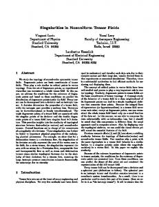
Figure 1. Elliptic umbilic points and their measured topological signature. Left frame: The simulated image (256 × 256 pixels) is given by the function L(x, y) = x 2 y + y 3 − 0.3y and is presented as a 3D plot. Right frame: The winding numbers ν in every image point are computed by taking a sum of the angle variations of the gradient vector along a rectangular contour of side-length 4 lattice units. Light dots correspond to singularities with ν = +2π while the dark ones represent ν = −2π .

Therefore, when t < 0 there are four singularities. Two of them (those with x = 0) are with topological number +2π and the other two have topological number −2π . They are presented in Fig. 1 for a negative value of the scale t. At t = 0, all four singularities annihilate in one point (x = y = t = 0). This process of annihilation is illustrated in the three-dimensional plot in Fig. 2. 5.3.

Two-Dimensional Hyperbolic Umbilic Point

In the next example no annihilation occurs. The two singular strings carry both current of −2π. Therefore, these singularities can be only scatter in the scale space as the total current cannot vanish. Consider the following solution of (1) in two dimensions: L(x, y, t) = x 2 y − y 3 − 4yt.

(48)

Singular points, defined as the points where ∂x L = ∂ y L = 0 are t < 0: x = 0; y = ±(−4t/3)1/2 t > 0: y = 0; x = ±2t 1/2 .

(49)

So both for t > 0 and t < 0 there are two singularities. The topological numbers are easily computed from (33) and are in this case ν = −2π for all

Figure 2. Three-dimensional plot of annihilation of singularity points in scale space. A cube of voxels presents the distribution of topological numbers in image defined in scale space by the function L(x, y, t) = x 2 y + y 3 + 8yt. The scale t is running along the vertical direction. Topological numbers at all scales (horizontal sections in the figure) are computed with rectangular contours with size 4 lattice spaces. They form four strings in the scale-space cube that annihilate at t = 0. Two strings (the dark ones) carry topological number of −2π and the other two (the light strings) represent singularity points with topological number +2π .

singularities at t 6= 0. Therefore, no annihilation is possible, the singularity strings scatter (see Fig. 3) at t = 0 and change their plane of “polarization” from x = 0 to y = 0. At the catastrophe point t = 0, the two singularities merge into a single, third-order singular

P1: TPR/NKD

P2: JSN/ASH/PCY

QC: JSN

Journal of Mathematical Imaging and Vision

264

KL645-04-Kalitzin

September 28, 1998

Kalitzin et al.

Figure 3. Three-dimensional plot of scatter of singularity points in scale space. A cube of voxels presents the distribution of topological numbers in image defined in scale space by the function L(x, y, t) = x 2 y − y 3 − 4yt. The scale t is running along the vertical direction. Topological numbers at all scales (horizontal sections in the figure) are computed with rectangular contours with size 4 lattice spaces. They form two strings in the scale-space cube that scatter at t = 0. At the scatter point the two saddle points merge into a degenerated singular point (the bright spot) with a winding number of −4π .

point with a winding number −4π. Thus exactly as the conservation law predicts. 6.

19:54

Topological Numbers and Causality

before the catastrophe. At the critical scale (in the example this is t = 0) the number of singularities is actually one (of a higher order though) and immediately after that there are two singularities. So the naive (strong) causality is broken. The number of singularities though, remains in this example effectively the same before and after the interaction. Our understanding of these form of causality is that only the complete scale space dynamics (for a finite scale interval) reveals whether the number of singularities increase, decrease, or remain the same. To give a more rigorous definition of this weaker causality principle, consider a closed hypersurface 6 in scale space surrounding a given top-point, such that there are no other top-points in the region enclosed by 6. Then the weaker causality requires that the number of singularities entering 6 is greater than the number of singularities leaving the hypersurface. All three examples above show causality in this sense (the first two are, of course, causal even in the strong sense). Having the distribution of singularities with their topological numbers in (20), we give now a quantitative measure for the difference between the number of singularity strings that enter a given region in scale space and the number of strings that leave this region. Recalling the definition of the current Jµ (41), we can replace the density (21) by the density X θ (x, t) = δ(x − x P (t)), (52) P

The last example of Section 5 shows that a naive causality principle, stating that in a linear diffusion scheme (1) the number of singularities can only decrease with the scale evolution, is not automatically true. In general, a strictly causal deformation will be one that yields at most one solution of the drift equation (39) for δt > 0 in any degenerate singular point. This is not the case when linear diffusion is assumed as an image evolution in d > 1. Indeed, in the last example of hyperbolic umbilic points we have for the drift equation: (δx)(δy) = 0,

(50)

(δx)2 − 2(δy)2 − 4δt = 0.

(51)

As already considered above, this gives two solutions both for δt > 0 and δt < 0. A weaker causality in this situation could mean that the number of singular points does not increase after a catastrophe has occurred in comparison to the state

where the sum is again over all singularities. Then we obtain the current ¡ ¢ K µ ≡ (K 0 , K i ) = θ (x, t) 1, −L i−1 j L0 j .

(53)

This new current measures the flux of singularities (of any charge ν) in a scale-space region Wd+1 . If we define the annihilation density κ(x, t) as: κ(x, t) = ∂ µ K µ ,

(54)

it will give us a measure of the distribution of those catastrophe points in scale space where annihilation (κ < 0) or creation (κ > 0) of singularities occurs. Regular points, nondegenerate singularities and catastrophe points where singularities only scatter will not contribute to the quantity (54). It is clear that the current (53) is not defined in the degenerate singularities. Nevertheless, the integral of the annihilation density (54) can be computed in a given scale-space

P1: TPR/NKD

P2: JSN/ASH/PCY

QC: JSN

Journal of Mathematical Imaging and Vision

KL645-04-Kalitzin

September 28, 1998

19:54

Topological Numbers and Singularities

region (neighborhood of the top-point of interest) as the total influx of the current K µ through a surface surrounding this region. In the expression (52), the winding numbers are replaced by 1 if the point is singular and by 0 if the scale-space point is nonsingular. Therefore, the information about the values of the singularities is filtered out. In practice, the density ν(x, t), is used by applying formula (20) to localize the singularities and their trajectories in scale space. Finally, we can formulate our weak causality principle with the condition: κ(x, t) ≤ 0 in any scale-space point. While preparing the manuscript of this paper, we were informed that the current (53) is considered also in [17] for analyzing the top-points characteristics in scale space.

7.

Summary and Discussion on Possible Applications to Image Processing

In this article we introduced a quantity characterizing isolated singular points in scalar images of any dimensions. For one-dimensional signals this quantity reduces to a local extrema identifier and in two dimensions it reduces to the winding number of the gradient field around any point of the image. In summary, the properties of this topological quantity are Discrete: It takes only a discrete set of values. Localized: It is zero in regular points and nonzero in the singularities. Nonperturbative: It can be operationally defined and nonperturbatively calculated using hypersurface integrals of the normalized gradient vector around the image point. Conserved: Under smooth image deformations, including Gaussian blurring, the topological density obeys a conservation law. Invariant: It is a topological quantity in the sense that homotopic deformations of the surfaces on which this quantity is computed do not affect its value (unless other singularities are crossed). Additive: The sum of topological numbers in a given region is a sum of these numbers in each subregion. These properties enabled us to explore the singularity structure of an image in the full range of scales. The localization property gives a practical tool to trace

265

the drift and the interactions of the singularities in scale space. The conservation property provides a nonperturbative insight to the possible outcomes of the interactions between the singular points. An illustrative example for the localization and scale-evolution properties of the topological number considered in this work is given with Fig. 4. Two texture patterns (check-board images with different wavelength) are superimposed (with different weights) and their scale-space evolution is studied. The first observation we want to stress out from Fig. 4 is the nonlinear feature of the invariant (7). Although frame 1 Fig. 4B is a linear superposition of the two patterns in Fig. 4A, the topological number distribution is not. Second, after the Gaussian blurring, the image in frame 4 reveals the same topological signature as the dominant texture (the one taken with a larger weight) from frame 1 in Fig. 4A. This suggests the possibility of a scale-classification of the texture patterns by means of their topological signatures evolving with scale. A second applied area, where we can speculate about the use of the topological numbers and their smooth evolution with scale, is the image segmentation realm. As shown in Fig. 5, singularities, localized with their winding numbers in a 2D image, determine a hierarchy of subobjects labeled by singularities with positive topological charge (extrema). It is plausible also to suggest, that at the borders between the subobjects, singularities with negative charge (7) (saddle points) are found. A comprehensive algorithm for such deepstructure segmentation will involve tracing the object hierarchy from large, down to finer scales and transferring the object labels to their subobjects. This method is now under investigation [18] and it involves techniques beyond the scope of the current paper. In this article we used the topological number (7) defined by the normalized gradient vector field. The same definition can be directly applied to singularities of any vector field. More generally, there are applications where the local orientation structure is defined not by a vector field, but by the Principal directions of a structural tensor. It would be interesting to extend the notion of a topological number to those cases. We were able to define a winding number associated with the principle direction in the two-dimensional case. In comparison with the vector winding number considered in Section 3.2, the winding number of the structural tensor is a multiple of π . This is due to the fact that the principle direction of the structural tensor has no orientation on it.

P1: TPR/NKD

P2: JSN/ASH/PCY

QC: JSN

Journal of Mathematical Imaging and Vision

266

KL645-04-Kalitzin

September 28, 1998

19:54

Kalitzin et al.

Figure 4. Scale-space texture evolution and its measured topological signature. A. Two checkerboard type of textures are generated as 256 × 256 pixel images. The upper part of frames 1 and 2 represent the simulated images and the lower part the corresponding topological number distributions. B. Frame 1: A linear superposition of the images in Fig. 4A (L 1 and L 2 ) is build according to the formula L 1 + 0.5L 2 where both components are normalized in the grey-scale range [−1, 1]. Frames 2 to 4: The image on frame 1 is blurred with scales t = 8, 10 and 14 correspondingly. Frames 5 to 7: Topological number distributions of the images in frames 1 to 4 correspondingly.

Another direction for further research can be aimed at finding an adequate topological or geometrical quantity characterizing in a nonperturbative way the structure of the top-points in scale space. A possible candidate is the density (54), but it is defined “at hoc” from a geometrical point of view. It may be interesting to analyze and compare the different diffusion

schemes in terms of this characteristic quantity of their top-points. Acknowledgments This work is carried out in the framework of the research program Imaging Science, supported by

P1: TPR/NKD

P2: JSN/ASH/PCY

QC: JSN

Journal of Mathematical Imaging and Vision

KL645-04-Kalitzin

September 28, 1998

19:54

Topological Numbers and Singularities

267

Figure 5. Scale-space evolution of a grey-scale image and its topological signature. Left column: A CT-scan image of 256 × 256 pixels is blurred with four different scales. Middle column: The topological number distribution is computed with rectangular contours of size 4 pixels in every image point. Right column: Combined stack of images representing the scale evolution of the image together with its topological number distribution. Extrema (white dots) label blob-type of formations while saddle points (black dots) are situated at the borders of the blobs.

the industrial companies Phillips Medical Systems, KLMA, Shell International Exploration and Production, and ADAC Europe. References 1. W.M. Boothby, An Introduction to Differential Geometry and Riemannian Geometry, Academic Press: New York, San Francisco, London, 1975.

2. T. Eguchi, P. Gilkey, and J. Hanson, “Gravitation, gauge theories and differential geometry,” Physics Reports, Vol. 66, No. 2, pp. 213–393, 1980. 3. L.M.J. Florack, B.M. ter Haar Romeny, J.J. Koenderink, and M.A. Viergever, “Images: Regular tempered distributions,” in Proc. of the NATO Advanced Research Workshop Shape in Picture—Mathematical Description of Shape in Greylevel Images, Ying-Lie O, A. Toet, H.J.A.M. Heijmans, D.H. Foster, and P. Meer (Eds.), Volume 126 of NATO ASI Series F, SpringerVerlag: Berlin, 1994, pp. 651–660.

P1: TPR/NKD

P2: JSN/ASH/PCY

QC: JSN

Journal of Mathematical Imaging and Vision

268

KL645-04-Kalitzin

September 28, 1998

19:54

Kalitzin et al.

4. P. Johansen, “On the classification of toppoints in scale-space,” Journal of Mathematical Imaging and Vision, Vol. 4, No. 1, pp. 57–68, 1994. 5. M. Kass, A. Witkin, and D. Terzopoulos, “Snakes: Active contour models,” in Proc. IEEE First Int. Comp. Vision Conf., 1987. 6. J.J. Koenderink, “The structure of images,” Biol. Cybern., Vol. 50, pp. 363–370, 1984. 7. T. Lindeberg, “Scale-space behaviour of local extrema and blobs,” Journal of Mathematical Imaging and Vision, Vol. 1, No. 1, pp. 65–99, March 1992. 8. T. Lindeberg, Scale-Space Theory in Computer Vision, The Kluwer International Series in Engineering and Computer Science, Kluwer Academic Publishers: Dordrecht, The Netherlands, 1994. 9. J. Milnor, Morse Theory, Volume 51 of Annals of Mathematics Studies, Princeton University Press, 1963. 10. M. Morse and S.S Cairns, Critical Point Theory in Global Analysis and Differential Topology, Academic Press: New York and London, 1969. 11. M. Nakahara, Geometry, Topology and Physics, Adam Hilger: Bristol and New York, 1989. 12. A.H. Salden, “Invariant theory,” in Gaussian Scale-Space Theory, J. Sporring, M. Nielsen, L.M.J. Florack, and P. Johansen (Eds.), Kluwer Academic Publishers, 1997. 13. A.H. Salden, B.M. ter Haar Romeny, and M.A. Viergever, “Local and multilocal scale-space description,” in Proc. of the NATO Advanced Research Workshop Shape in Picture—Mathematical Description of Shape in Greylevel Images, Ying-Lie O, A. Toet, H.J.A.M. Heijmans, D.H. Foster, and P. Meer (Eds.), Volume 126 of NATO ASI Series F, Springer-Verlag: Berlin, 1994, pp. 661–670. 14. A.H. Salden, B.M. ter Haar Romeny, and M.A. Viergever, “Algebraic invariants of linear scale spaces,” Journal of Mathematical Imaging and Vision, March 1996 (submitted). 15. A.H. Salden, B.M. ter Haar Romeny, and M.A. Viergever, “Differential and integral geometry of linear scale spaces,” Journal of Mathematical Imaging and Vision, May 1996 (submitted). 16. B.M. ter Haar Romeny (Ed.), Geometry-Driven Diffusion in Computer Vision, Kluwer Academic Publishers: Dordrecht, 1994. 17. L.M.J. Florack, Detection of Critical Points and Top-Points in Scale-Space. In preparation. 18. S.N. Kalitzin, B.M. ter Haar Romeny, and M.A. Viergever, “On topological deep-structure segmentation,” submitted for ICIP’97, Santa Barbara.

Stiliyan N. Kalitzin received a master degree in Nuclear Physics and Nuclear Technology from the University of Sofia, Bulgaria. He

has worked in the Institute for Nuclear Research in Sofia and in the Joint Institute for Nuclear Research in Dubna, Russia. In 1988 he obtained a Ph.D. in Theoretical and Mathematical Physics on the subjects of Supersymmetry and Supergravity. Since 1990, Stiliyan Kalitzin hold several consecutive post doctoral positions in different academic institutes in the Netherlands. His current research interests are natural and automated perceptual grouping, neural networks, differential geometry, pattern recognition and nonlinear scale-space theories. Since 1996, Stiliyan Kalitzin works in the Image Sciences Institute at the University of Utrecht.

Bart M. ter Haar Romeny received a M.S. in Applied Physics from Delft University of Technology in 1978, and Ph.D. from Utrecht University in 1983. After being the principal physicist of the Utrecht University Hospital Radiology Department. He joined in 1989 the Utrecht University 3D Computer Vision Research Group where he is an Associate Professor. He is member of the editorial board of JMIV. His interests are mathematical aspects of front-end vision, in particular, linear and nonlinear scale-space theory, medical computer vision applications, picture archiving and communication systems, differential geometry and perception. He authored several papers and book-chapters on these issues, edited a recent book on nonlinear diffusion theory in Computer Vision and is involved in (resp. initiated) a number of international collaborations on these subjects.

Alfons H. Salden received a M.Sc. in Experimental Physics in 1992 and a Ph.D. in 1996 both from utrecht University. His main research interests are scale-space theories, invariant theory, differential and integral geometry, theory of partial differential and integral equations, topology and category theory.

P1: TPR/NKD

P2: JSN/ASH/PCY

QC: JSN

Journal of Mathematical Imaging and Vision

KL645-04-Kalitzin

September 28, 1998

19:54

Topological Numbers and Singularities

269

The Netherlands. His research topics included hierarchical methods for image segmentation and mathematical morphology. Currently, he is working for Shell International Exploration & Production BV, in the field of 3D seismic interpretation research.

Peter FM Nacken has masters degrees in Mathematics and Theoretical Physics from the University of Nijmegen, The Netherlands, and a Ph.D. in Computer Science from the University of Amsterdam,

Max A. Viergever