38th Euromicro Conference on Software Engineering and Advanced Applications September 5-8, 2012 copyright IEEE
Towards a model-based approach for allocating tasks to multicore processors Juraj Feljan, Jan Carlson M¨alardalen Real-Time Research Centre M¨alardalen University V¨aster˚as, Sweden
[email protected],
[email protected]
Abstract—Multicore technology provides a way to improve the performance of embedded systems in response to the demand in many domains for more and more complex functionality. However, increasing the number of processing units also introduces the problem of deciding which task to execute on which core in order to best utilize the platform. In this paper we present a model-based approach for automatic allocation of software tasks to the cores of a soft real-time embedded system, based on design-time performance predictions. We describe a general iterative method for finding an allocation that maximizes key performance aspects while satisfying given allocation constraints, and present an instance of this method, focusing on the particular performance aspects of timeliness and balanced computational load over time and over the cores. Keywords-embedded systems; multicore; soft real-time; task allocation; performance analysis; architecture optimization; model-based development;
I. I NTRODUCTION Computers have become prevalent in our daily lives, as they are used in industry, business, education, research, traffic, entertainment etc. Most computer systems are embedded systems, i.e., microprocessor based systems with dedicated functions, embedded in and interacting with a larger device. Embedded systems are getting more and more performance intensive as they include more functionality than ever, while at the same time having to be reliable, flexible, maintainable and robust. Similarly to general purpose computer systems, there is a trend to tackle the increasing performance demands of embedded systems by increasing the number of processing units. An example is the use of multicore processors, i.e., a single chip with two or more processing units (cores) coupled tightly together to increase processing power while keeping power consumption reasonable. While providing a higher performance capacity, this also introduces the problem of how to best divide the software functionality between the cores. One way of determining whether a particular allocation of functionality to the cores yields satisfactory performance is implementing, deploying and running the system in order to obtain performance measurements. However, this method is time consuming and thus costly, and a preferred approach would be to predict performance
Tiberiu Seceleanu ABB Corporate Research V¨aster˚as, Sweden
[email protected]
at a reasonable accuracy early in the development process, prior to the implementation. Performance is a broad concept and there are many characteristics that influence whether an allocation is qualified as good or bad, including for example response time of some critical functionality, energy consumption, and control quality, but also concerns such as safety, security, availability, scalability and robustness. The primary domain addressed in this work is soft real-time embedded systems, i.e., systems where timing is crucial to the correctness of a system but occasional deadline misses can be tolerated. Thus, one performance aspect particularly relevant for this domain is average timeliness, as compared to worst-case timeliness which is typically in focus for hard real-time systems where absence of deadline violations must be guaranteed. In this paper we present a model-based approach for allocating software tasks onto the cores of a soft realtime embedded system, based on local search guided by performance simulations. We outline the envisioned general approach and exemplify it by focusing on two particular performance metrics, namely the number of deadline misses and the distribution of computational load over time and over the cores. The motivation for preferring allocations where computation is evenly distributed over time and over the cores is to minimize the impact of future modifications on the temporal behavior of the system. Since the performance metrics of interest depend heavily on the dynamic interplay between tasks, and since we are focusing on average performance rather than a worst-case scenario, they are not easily derived analytically from task parameters. Instead, we base the search for appropriate allocations on simulations of the allocation candidates. The paper is organized as follows. Section II presents an overview of the proposed method. Then, in Section III we detail the four activities of the method in separate subsections, illustrated by a running example. We also describe how the activities together contribute to an iterative cycle of searching for a good allocation of tasks to cores. In Section IV we apply the method to a more complex example. Section V surveys related work before Section VI presents future work and concludes the paper.
Functional design
Architectural model
Affinity specification
Model transformation
Simulation model Allocation optimization
Simulation
Simulation results
Performance analysis
Allocation
Figure 1.
The allocation optimization process
II. M ETHOD OUTLINE In this section we outline the proposed model-based method for obtaining an allocation of software tasks onto the cores of a soft real-time multicore system. We propose an iterative approach based on local search, where each iteration makes a small modification to the best allocation found so far, and determines by means of simulation if the modification resulted in an improvement or not. Figure 1 shows the activities (depicted by rounded rectangles) and artefacts (depicted by rectangles) that constitute the method. The main input to the allocation optimization is an architectural model, built by the system designer as part of the manual functional design activity. This model provides an architectural specification of the system as a collection of software tasks and the connections between them. Additionally, an architectural model contains information about the hardware platform. An affinity specification defines the affinity of each task, i.e. the parameter which tells to which of the cores the task will be allocated. An initial affinity specification candidate can be provided by the system designer. In the model transformation activity, a simulation model is generated from the architectural model by means of an automatic model-to-model transformation. A simulation model captures the dynamic interaction between the tasks on the same or different cores, as specified by the affinities, including task scheduling and the delays in transfer of data and control. In the next step, simulation is performed. Finally, the performance analysis processes the data collected during
simulation and derives from it a few concrete performance metrics by which the current allocation candidate can be compared against others. The result of the performance analysis is a new affinity specification candidate — constructed by making a small modification to the best allocation found so far — that is fed back to the model transformation activity. This forms an allocation optimization cycle that repeats the model transformation, simulation and performance analysis activities in search for an affinity specification that yields good performance. When the iteration stops, the method outputs the best affinity specification it was able to find, to be used in subsequent activities of implementation. Support for architectural modeling, model transformation and simulation has been implemented in Mathworks MATLAB and Simulink [1], two integrated products that are a de-facto modeling standard in industry. The overall optimization, including the performance analysis, has been implemented as a Java program invoked from within the Mathworks environment. III. O PTIMIZING ALLOCATION OF TASKS TO CORES In this section we detail the activities of the proposed approach. For each of them, we first give a general description of the activity and the corresponding artefacts, and then the activity is illustrated using a running example focusing on two particular performance aspects, namely deadline misses and the distribution of computational load over time and over the cores. After detailing the individual activities, we describe how they are combined together to form an iterative cycle of searching for a good allocation of tasks to cores. A. Functional design Functional design represents the complex manual activity of defining the structure of the system being developed. As input to our process, we use one of the artefacts created in the functional design activity, an architectural model. It specifies the system as a collection of tasks and the connections between them, in the form of a Simulink model. The model blocks representing the tasks are reused from our custom Simulink library. We support both periodic and event-driven tasks. Each task has the following parameters specified as part of the functional design by the system designer: best-case execution time, worst-case execution time, the size of data produced during each execution of the task. Additionally, periodic tasks have a parameter defining their period. Apart from the software specification of the system in the form of tasks, an architectural model holds some information related to the hardware platform, such as the number of cores, communication delay parameters and scheduling options (for more details, see Section III-B). The initial specification of the affinities is optional (indicated by the dashed line in Figure 1). It can be provided
dataIn
affinity: 1 period: 25 BCET: 5 dataOut WCET: 8 send: 3
dataIn
T1
dataIn
affinity: 2 period: 50 BCET: 4 dataOut WCET: 6 send: 5
T2
dataIn
T4
Figure 2.
affinity: 1 BCET: 3 dataOut WCET: 5 send: 2
dataIn
affinity: 2 BCET: 8 dataOut WCET: 10 send: 0 T3
affinity: 2 BCET: 3 dataOut WCET: 4 send: 0 T5
An example of an architectural model
by the system designer in the form of affinity values, affinity constraints or a combination of the two. An affinity value simply specifies to which of the cores a task will be allocated initially. An affinity constraint specifies a more complex affinity rule that must be satisfied for all allocation candidates considered during the iteration. For instance, the system designer can define that a particular task can be allocated only to a subset of the available cores, or that two tasks must be allocated to the same core, or to different cores. Should the system designer choose not to provide the initial specification of affinities, a random specification is generated. The subsequent affinity specifications result from the performance analysis activity. Example: In order to illustrate the optimization process, we introduce a running example. We start by presenting an example of an architectural model (Figure 2). It is a Simulink model consisting of 5 tasks, named T 1 to T 5. T 1 and T 4 are periodic tasks, while the other three are event-driven tasks triggered by data being available, as seen from the connections between the tasks in the figure. The tasks have the aforementioned parameters specified: the bestand worst-case execution time (BCET and WCET), the size of produced data, and the period for periodic tasks. Additionally, the initial affinity specification is given in the form of affinity values stored as task parameters, since the current implementation does not explicitly separate an affinity specification from an architectural model. The hardware related information in the example is defined as follows. The system has two cores, core1 has a preemptive scheduler and core2 a nonpreemptive scheduler. Local memory delay is set to 1 time unit and global memory delay to 2. This information is stored as model parameters and it is therefore not visible from the figure. B. Model transformation The first step in each iteration of the allocation optimization cycle is the model transformation activity, which generates a simulation model from the architectural model and the current affinity specification, by means of an automatic transformation. The purpose of a simulation model is to capture all aspects of performance that influence the quality
of a particular allocation, such that simulation can be performed, and that the simulation results become available for analysis. This means on one hand enriching the architectural model with behavior that influences performance, and on the other hand abstracting away the details from the architectural model that do not affect the particular performance aspect we are considering. A simulation model is a hierarchical model, as the task blocks are placed within core blocks, according to the affinity specification. As mentioned in Section I, we are interested in the distribution of computational efforts over the cores and over time. Therefore, we need a simulation model to capture both the interference from the tasks on the same core that are ready to execute at the same time, and the differences in delays caused by data being transferred between tasks on the same and different cores, respectively. Task interference is addressed by a scheduler block in each core, governing the execution order of the tasks allocated to that core. The behavior of the task- and scheduler blocks is implemented by MATLAB programming language code automatically generated as part of the model transformation. A task can be in one of the following three states: waiting, ready, or executing. A task is in the waiting state while it waits for a trigger, either a periodic signal for periodic tasks or an event for event-triggered tasks. Upon being triggered, the task transitions to the ready state and raises its request signal to the scheduler. When the task is granted access to the processor, represented by a grant signal from the scheduler, it reduces its remaining execution by one time unit. When the remaining execution reaches zero, the task returns to the waiting state. This structure allows for both preemptive and nonpreemptive schedulers to be defined, since a scheduler decides which task to grant execution rights at each simulation step. If a task has not finished executing when the next triggering occurs, it is considered to have missed its deadline. Deadline misses are reported to the scheduler and stored in the simulation results. The delays caused by data communication depend on the architecture of the cores. If there is only global memory shared between the cores, the communication cost is the same regardless of whether the data is communicated locally or remotely. If, however, the cores have local memory, then a higher cost is paid for remote communication than for local communication. In both cases, the communication cost is proportional to the amount of data being communicated. As mentioned in Section III-A, information about the number of available cores, the scheduler used by the different cores, whether the cores have local memory, and the relation between the times necessary to access localand global memory, is specified by the system designer and stored as parameters of the architectural model. This information is forwarded to the simulation model during the model transformation.
T2_dataOut
load
load T3_dataIn execution execution misses
misses
core1
core2 Mux
sim_results
(a)
load
grant
dataIn 1 T2_dataIn
1 load
affinity: 2 request BCET: 8 WCET: 10 dataOut send: 0 miss
add
Mux
T3
grant
dataIn
load affinity: 2 period: 50 request BCET: 4 WCET: 6 dataOut send: 5 miss
request
Mux
miss
Demux
deadlineMisses
3 misses
scheduler
load
grant
grant
fcn
T4
dataIn
Mux
2 execution
affinity: 2 request BCET: 3 WCET: 4 dataOut send: 0 miss T5
(b) Figure 3.
An example of a simulation model
Example: Figure 3 depicts the simulation model generated from the architectural model in Figure 2. Figure 3a shows the top level of the simulation model, with the two core blocks and additional utility blocks that enable storing and viewing simulation results. In Figure 3b we dive one level deeper into the hierarchy and show the internals of core2 (core1 is structured in a similar way). According to the initial affinity specification, tasks T 3, T 4 and T 5 are allocated to this core. Apart from the ports present in the architectural model, all task blocks in the simulation model have additional ports. The ports named request and grant enable the scheduler block to control task execution, while the load port communicates the remaining task execution (more details are given in Section III-C). The miss port
is used to communicate when a task misses its deadline. The multiplexer/demultiplexer blocks shown in Figure 3b are used to make a vector from the individual signals, and vice versa, to simplify the scheduler implementation. C. Simulation In this step, the simulation model is executed in order to collect relevant performance data characterizing the allocation. The simulations are not deterministic, since the execution time of each task instance is randomly selected in the interval defined by the best- and worst-case execution time parameters. In order to ensure that average performance aspects are properly represented, the simulation time should not be shorter than the duration of several hyperperiods of
Execution time
18 15 12 9 6 3 0 0
T3 T4 T5
20
40 60 Simulation time
80
100
80
100
Load
(a)
18 15 12 9 6 3 0 0
20
40 60 Simulation time (b) Figure 4.
Simulation results for core2
all tasks in the system. As discussed previously, in addition to timeliness (represented by the number of missed deadlines), we are interested in how the computational load is distributed over time on the different cores. The computational load over time of a core is represented by a line graph of the load values at the beginning of each simulation step (a simulation step corresponds to a clock cycle). In the beginning of a particular clock cycle, the load value is equal to the sum of the remaining execution times of the tasks that are ready to execute. In a particular clock cycle, the load can be influenced in the following ways. First, if no task ready for execution exists in the beginning of a particular clock cycle, the load stays at zero in this particular clock cycle. Second, if a task that became ready for execution in a previous clock cycle has remaining execution time at the beginning of a particular clock cycle, the load decreases by one in this particular clock cycle. The decrease of the load by one corresponds to one task having processor access in one clock cycle. Third, if a task, or several tasks get ready for execution in the beginning of a particular clock cycle, the load increases in the beginning of this particular clock cycle by the sum of the execution times of all tasks that got ready for execution. A combination of the two latter cases can happen in the same clock cycle. Informally, load at a particular time is the amount of the remaining scheduled execution. To account for the delay due to data communication, we model the cost of data transfer (the communication cost) by adding it to the execution time of the receiving task. Whenever a task becomes ready, a new execution time is generated as a random value between the task’s bestand worst-case execution times. The communication cost is added to this generated value, producing the total execution
time of this task instance. As mentioned in Section III-B, the communication cost depends on the size of data and whether the data comes from a local or remote task. The information collected from the simulation are the load values and the deadline misses, for each core at each simulation step. It is also possible to view a trace of the execution of the tasks. Example: Figure 4 shows the results of simulating the model depicted in Figure 3. In Figure 4a the task execution trace is shown, while Figure 4b shows the computational load trace, both for core2. We can observe the following from the figure. When a task becomes ready, it contributes its execution time to the load of its core. When a task is executed, it reduces the core load, one unit per clock cycle. For instance, at simulation time 50, task T 4 becomes ready with an execution time of 5. This is added to the core load, while one load unit is subtracted by T 3 that is executing at that point. As described above, tasks receiving data pay the cost of the data transfer. For instance, task T 3 receives 2 data units from T 2 located on core1. The execution time of T 3 (a random value between its BCET and WCET) is increased by 4 units of data transfer cost (2 data units multiplied by the delay of reading global memory), making its total execution time. For T 5, receiving data from T 4 which is located on the same core, the communication cost is 5 (5 data units multiplied by the delay of reading local memory). The scheduler on core2 is nonpreemptive, meaning that once a task is granted access to the processor if will execute until it is finished, regardless of other tasks that are ready simultaneously. This can, for instance, be observed between time steps 50 and 55, where T 3 and T 4 are both ready, and T 4 has to wait for T 3 to finish its execution.
D. Performance analysis In the performance analysis activity the simulation data is filtered into a format that allows a straightforward comparison of allocations, in order to compare the current allocation to the best allocation found in the previous iterations. The performance analysis activity also generates a new affinity specification candidate, based on the currently best alternative, to be used in the next iteration. In our current instance of the optimization method, allocations are compared with respect to two criteria, feasibility and maximum peak load. An allocation is feasible if the deadline misses remain below a certain limit (e.g., at most 2% of the task executions miss their respective deadline). The maximum peak load of an allocation is the maximum load reached on any core during the simulation. Concretely, allocations A1 and A2 are compared in the following way. If A1 is infeasible, A2 is better if it has fewer deadline misses than A1. If allocation A1 is feasible, allocation A2 is better if A2 is feasible and if the maximum peak load of A2 is lower that the maximum peak load of A1. Alternatively, it is possible to define a fitness function that takes deadline misses and maximum peak load as input and outputs a single value specifying the quality of a particular allocation, making it easy to compare two allocations. The generation of a new allocation candidate from the currently best one can be done in a purely random way, but it is also possible to use information from the analysis to guide the modification. In our case, the modification of an infeasible allocation is done by just randomly reallocating one task to a new core. For feasible allocations, however, we try to decrease the peak load by relocating a random task from the core with the highest peak load to a random other core. Example: The peak load value on core1 is 8 and the peak load on core2 is 18 (it occurs at time 64 in Figure 4b). This makes the maximum peak load of the allocation 18. No deadline misses are recorded during the simulation, so the allocation is feasible. For simplicity, we use 0% deadline misses as the feasibility limit in the example. Because this is the first allocation we evaluate, and thus the best so far, it will be the basis for the next allocation. Since it is feasible, one of the tasks currently allocated to core2 will be randomly selected and instead allocated to core1 in the affinity specification to be used in the second iteration. E. The optimization cycle The analysis activity in one iteration of the process compares two allocations, stores the better one, and proposes a new allocation that will be tested in the next iteration. When generating a new allocation, it must be checked against the affinity constraints to make sure that they are satisfied by the new allocation. The new affinity specification is fed as input to the new iteration of the process, or more specifically,
to the model transformation activity. This forms the allocation optimization cycle based on local search that in each iteration makes a modification to the affinities, evaluates the result and continues with the affinity specification that was identified as best so far. In other words, the allocation optimization repeats the model transformation, simulation and performance analysis activities in search for an affinity specification that yields the best possible performance. The iteration continues until a particular number of consecutive iterations has not resulted in a better allocation. In order to avoid getting stuck in a local optimum, the whole procedure is repeated several times, starting from a different initial affinity specification each time. Example: Continuing the example, a new affinity specification A2 was created by relocating task T 5 (randomly selected from the tasks on the core with the highest peak load) to core1 (a random other core). Repeating the transformation, simulation and performance analysis for the new affinity specification resulted in a maximum peak load of 20 (on core1), with no deadline misses. Since this allocation is worse than A1, A1 is kept as the best allocation, and the process continues with a new allocation, A3, based on A1. IV. E XAMPLE In this section we present an experiment where our allocation optimization approach is applied to a more realistically sized system in order to test the scalability of the method. We use a relatively complex architectural model consisting of 17 tasks (6 periodic and 11 event-triggered). As shown in Figure 5, the tasks are organized in three main task chains where a periodic task triggers a number of event-driven tasks. Additionally, there are three independent periodic tasks that do not trigger other tasks. The hardware platform consists of three cores, and all three cores are assigned a nonpreemptive scheduler. The local memory delay is defined as 1 time unit and the global memory delay as 3 time units. For three cores and seventeen tasks, the number of possible allocations is 317 = 129 140 163. The allocation optimization was run with parameters 50 and 20, representing that the search is restarted 50 times with random initial affinity specifications, and that each search should continue until there are 20 consecutive iterations without improvement. The simulation length was set to 300 time units (the hyperperiod of the tasks is 50). With this setup, the allocation optimization took just under 100 minutes on a PC with an Intel i5 dual-core CPU clocked at 2.7GHz. In total, 1989 iterations were performed, which means that a search on average required 40 iterations before reaching the termination criterion of 20 consecutive iterations without improvement, and each iteration took around 3 seconds. The result of the optimization is a feasible allocation with a maximum peak load of 14 time units. Of the 50 restarted
dataIn
affinity: 3 period: 50 BCET: 5 dataOut WCET: 7 send: 2
dataIn
T01
affinity: 3 BCET: 2 dataOut WCET: 3 send: 2
dataIn
T02
dataIn
T03
affinity: 2 BCET: 1 dataOut WCET: 3 send: 2
dataIn
T04
dataIn
affinity: 1 period: 25 BCET: 5 dataOut WCET: 10 send: 3
dataIn
T08
dataIn
T12
dataIn
affinity: 3 BCET: 1 dataOut WCET: 3 send: 2
dataIn
T05
affinity: 1 BCET: 3 dataOut WCET: 5 send: 1
dataIn
T09
affinity: 1 period: 25 BCET: 2 dataOut WCET: 3 send: 2
affinity: 1 BCET: 2 dataOut WCET: 4 send: 0
affinity: 3 BCET: 3 dataOut WCET: 5 send: 1
T13
dataIn
affinity: 1 BCET: 1 dataOut WCET: 2 send: 0 T14
Figure 5.
dataIn
T06
dataIn
T10
affinity: 3 BCET: 1 dataOut WCET: 2 send: 1
affinity: 2 BCET: 3 dataOut WCET: 4 send: 2
affinity: 1 BCET: 3 dataOut WCET: 5 send: 0 T07
affinity: 1 BCET: 3 dataOut WCET: 5 send: 0 T11
dataIn
affinity: 2 period: 25 BCET: 2 dataOut WCET: 4 send: 0
dataIn
T15
affinity: 3 period: 25 BCET: 2 dataOut WCET: 4 send: 0 T16
dataIn
affinity: 1 period: 25 BCET: 1 dataOut WCET: 2 send: 0 T17
The architectural model used in the example
searches, 17 found a feasible allocation, and 10 of these have a peak load lower than 20. V. R ELATED WORK There has been substantial research on scheduling for multicore real-time systems, which includes as a subproblem the allocation of tasks to cores. The approaches can be grouped into partitioning (where tasks are statically allocated to the cores, and each core has its own scheduler), global scheduling (where tasks can move between the cores according to a global scheduler) and hybrid scheduling (a combination of the two). Our approach belongs to the former group, task partitioning, which is analogous to a bin packing problem, proven to be NP hard, meaning that finding an optimal allocation in polynomial time is not realistic in the general case [2]. Therefore the approaches for task allocation typically use heuristics in search for near-optimal solutions. Here we give a couple of examples. Dhall and Liu [3] describe two scheduling mechanisms, rate monotonic next fit scheduling and rate monotonic first fit scheduling, that try to assign the tasks to the cores using the next fit and first fit heuristic, respectively, while keeping each core schedulable according to rate monotonic scheduling. Nemati, Nolte and Behnam [4] present a partitioning algorithm that allocates a task set on a multicore platform such that the total amount of task blocking time is reduced. Most approaches for scheduling multicore real-time systems target hard real-time systems, but Devi specifically focuses on soft real-time multicore systems [5]. However, her approach uses global scheduling, and, similarly to the hard real-time approaches, is based on schedulability analysis and focuses on the worst case, while our approach relies on simulation and focuses on the average case. Model-based approaches for performance predictions, such as DeepCompas, TrueTime or Palladio, form another
field of related work. DeepCompas [6] is an analysis framework for predicting performance related properties of component-based real-time systems. It combines models of individual software components and hardware blocks to produce an executable model of the system. By simulating this model, performance predictions are obtained. DeepCompas also supports trade-off between several architecture alternatives. TrueTime [7] is a Simulink toolbox for simulation of distributed real-time control systems. It enables simulation of the temporal behavior of a multitasking real-time kernel executing controller tasks, and of medium access and packet transmission in a local area network. Palladio [8] is an approach for early performance predictions of componentbased software architectures of business information systems, but can also be used to model embedded systems. The key feature of Palladio is the parameterized component quality-of-service specification called resource demanding service effect specifications. These specifications abstractly model the performance related information for components (for example, how a provided service calls the required services of a component, resource usage, transition probabilities, loop iteration numbers and parameter dependencies) to allow accurate performance predictions. Additional approaches are presented in Koziolek’s survey [9]. However, in contrast to our work, none of these approaches focus on soft-real time multicore systems. Architecture optimization is another area of related work. Grunske et al. [10] present a survey of methods for optimizing dependability, cost and performance attributes of real-time embedded systems. A more recent approach is ArcheOpterix [11], a framework for optimizing software architectures modeled in AADL (Architecture Analysis and Description Language). The quality attributes supported by the approach include reliability, performance and energy. ArcheOpterix can be extended to any other quality attribute
for which quantitative prediction for AADL is available. PerOpteryx [12] is a framework for optimizing componentbased software architectures, based on model-based quality prediction techniques. Its distinctive feature is the extensible degrees of freedom model. A degree of freedom is a modifiable aspect of a software architecture that the optimization process is allowed to change in search for good architecture candidates. Conceptually, PerOpteryx is independent of the considered quality attributes, software architecture metamodeling language, and degrees of freedom, while the current implementation is based on Palladio. Again, none of these methods are tailored specifically for soft-real time multicore systems. SimTrOS and MacSim are examples of related work on simulating real-time multicore systems. SimTrOS [13] is a real-time multicore simulator for evaluating resource locking protocols. MacSim [14] is a simulator for embedded realtime systems with a large number of cores. Both approaches focus on hard-real time. VI. C ONCLUSION AND FUTURE WORK We have presented our approach for tackling the problem of allocating software tasks to the cores of a multicore system. The approach targets soft real-time embedded multicore systems, and is based on an iterative model-driven optimization cycle which performs a simulation guided local search for an allocation that yields good average-case performance. We have illustrated the general approach by focusing on two particular performance aspects relevant for soft realtime systems, namely timeliness and the distribution of computational load over time and over the cores. As the next step we intend to validate the approach in a case study, including a validation of the simulation model by comparing the resulting performance predictions against measured performance of a real system. Based on the results of the validation, we plan to refine the initial simulation model in order to have a more fine-grained view of the task interaction during simulation, in particular with respect to the modeling of communication between and within cores. Moreover, the architectural modeling should be extended with support for new constructs such as separation of data and triggering, tasks receiving data from multiple sources, and task synchronization over shared resources. After the validation, we will investigate additional performance aspects, such as end-to-end response times and dynamic memory usage. The current model-to-model transformation is implemented with the MATLAB programming language. As the complexity of the architectural and simulation models increase, there will be a need for a more structured and maintainable approach, for example representing the Simulink models in the Eclipse Modeling Framework (EMF) format and implementing the transformation with a model transformation language such as QVT or ATL.
ACKNOWLEDGMENT This work was supported by the Swedish Foundation for Strategic Research via the Ralf 3 project, and by the Swedish Research Council project C ONTESSE (2010-4276). R EFERENCES [1] Mathworks MATLAB and Simulink, http://www.mathworks. com/, [Accessed: 2012-03-08]. [2] D. S. Johnson, “Near-optimal bin packing algorithms,” Ph.D. dissertation, Massachusetts Institute of Technology, 1973. [3] S. K. Dhall and C. L. Liu, “On a real-time scheduling problem,” Operations Research, vol. 26, no. 1, 1978. [4] F. Nemati, T. Nolte, and M. Behnam, “Partitioning RealTime Systems on Multiprocessors with Shared Resources,” in Proceedings of 14th International Conference On Principles Of Distributed Systems, 2010. [5] U. C. Devi, “Soft Real-Time Scheduling on Multiprocessors,” Ph.D. dissertation, University of North Carolina at Chapel Hill, 2006. [6] E. Bondarev, “Design-time performance analysis of component-based real-time systems,” Ph.D. dissertation, Eindhoven Universty of Technology, 2009. [7] A. Cervin, D. Henriksson, B. Lincoln, J. Eker, and K.-E. ˚ en, “How does control timing affect performance? AnalArz´ ysis and simulation of timing using Jitterbug and TrueTime,” Control Systems, IEEE, vol. 23, no. 3, 2003. [8] S. Becker, H. Koziolek, and R. Reussner, “The Palladio component model for model-driven performance prediction,” Journal of Systems and Software, vol. 82, no. 1, 2009. [9] H. Koziolek, “Performance evaluation of component-based software systems: A survey,” Performance Evaluation, vol. 67, no. 8, 2010, special Issue on Software and Performance. [10] L. Grunske, P. Lindsay, E. Bondarev, Y. Papadopoulos, and D. Parker, “An Outline of an Architecture-Based Method for Optimizing Dependability Attributes of Software-Intensive Systems,” in Architecting Dependable Systems IV, ser. Lecture Notes in Computer Science. Springer Berlin / Heidelberg, 2007, vol. 4615. [11] A. Aleti, S. Bjornander, L. Grunske, and I. Meedeniya, “ArcheOpterix: An extendable tool for architecture optimization of AADL models,” in ICSE Workshop on Model-Based Methodologies for Pervasive and Embedded Software, 2009. [12] A. Koziolek, “Automated improvement of software architecture models for performance and other quality attributes,” Ph.D. dissertation, Karlsruhe Institute of Technology, 2011. [13] J. Schneider, M. Bohn, and C. Eltges, “SimTrOS: A Heterogenous Abstraction Level Simulator for Multicore Synchronization in Real-Time Systems,” in WATERS in conjunction with ECRTS, 2011. [14] S. Metzlaff, J. Mische, and T. Ungerer, “A Real-Time Capable Many-Core Model,” in The 32nd IEEE Real-Time Systems Symposium, Work-in-Progress Session, 2011.