Bart Selman, Henry Kautz, and Bram Cohen. Local search strategies for satisfiabil- ity testing. In DIMACS Series in Discrete Mathematics and Theoretical ...
Towards Computing Revised Models for FO Theories Johan Wittocx? , Broes De Cat, and Marc Denecker Department of Computer Science, K.U. Leuven, Belgium {johan.wittocx,broes.decat,marc.denecker}@cs.kuleuven.be
Abstract. In many real-life computational search problems, one is not only interested in finding a solution, but also in maintaining it under varying circumstances. E.g., in the area of network configuration, an initial configuration of a computer network needs to be obtained, as well as a new configuration when one of the machines in the network breaks down. Currently, most such revision problems are solved manually, or with highly specialized software. A recent declarative approach to solve (hard) computational search problems involving a lot of domain knowledge, is by finite model generation. Here, the domain knowledge is specified as a logic theory T , and models of T correspond to solutions of the problem. In this paper, we extend this approach to also solve revision problems. In particular, our method allows to use the same theory to describe the search problem and the revision problem, and applies techniques from current model generators to find revised solutions.
1
Introduction
In many real-life search problems, one searches for objects of a complex nature, such as an assignment, a plan or a schedule. Often, these objects can be represented by a finite structure and implicitly described by a logic theory. This observation led to declarative problem solving paradigms based on finite model generation such as Answer Set Programming [6, 9], np-spec [2] and the Model Expansion framework [8]. Several efficient solvers for these frameworks have been developed, making them applicable in practice. Often, one is not (only) interested in a single solution to a search problem, but also in revising this solution under varying circumstances. E.g., a network administrator is interested in computing an initial configuration of a computer network as well as in maintaining the configuration when one of the machines in the network breaks down. Typically, the following are requirements for a revised solution: 1. To allow a fast reaction on new circumstances, computing a revision should be efficient. ?
Research assistant of the Fund for Scientific Research - Flanders (FWO-Vlaanderen)
2. Executing a proposed revision in the problem domain usually has a certain cost. E.g., it takes time to move mail servers from one computer to another. A good revision should preferably have a low cost. I.e., it should be executable by a small number of cheap operations. Most existing approaches to solve revision problems are tailored towards a specific application such as train rescheduling, and hence, they are not (entirely) declarative. In this paper, we present a revision method that is much closer to the declarative problem solving frameworks mentioned above. Formally, we describe a revision problem by a theory T , a finite model M of T and a set of atoms C: T describes the original search problem, M a solution to that problem and C the atoms that should swap truth value compared to M . A solution to the revision problem is a model M 0 of T such that for every atom in C, its truth value in M 0 is opposite to its truth value in M . Revision problems where the theory T or the domain of M is changed can be reduced to this case, as we show in Section 3.2. In this paper, we describe a method to solve revision problems where T is a first-order logic (FO) theory. Like finite model generation for FO, these problems can easily be reduced to SAT. An off-the-shelf SAT solver can then be used to solve the resulting SAT problem. However, directly using this approach does not satisfy the two requirements mentioned above. It does not guarantee that the revised model is close to the original model and it can take too much time and space to create and store the SAT problem. The method we propose avoids these problems by first constructing a set of atoms S 0 , called a search bound. The bound contains all the atoms that we allow to swap truth value to obtain a revised model M 0 from the original one M . Then the method tries to find, by reducing to SAT, such a revised model M 0 . If it does not succeed, the bound S 0 is enlarged and the process is repeated. However, if it succeeds and S 0 is relatively small, the two requirements are met. Only a small number of operations should be performed to obtain M 0 , because the only changes are on atoms in S 0 . Also, reducing to SAT can be efficient if S 0 is small. To make the approach work, the consecutive search bounds should be constructed such that there is a reasonable chance that a revised model bounded by them exists. In Section 5, we present a non-deterministic algorithm to compute such search bounds. Experiments with a prototype implementation are discussed in Section 6. They indicate that the algorithm often finds small search bounds containing a revision. We end with conclusions and topics for future work.
2
Preliminaries
We assume the reader is familiar with classical first-order logic (FO), see, e.g., [4]. We introduce the conventions and notations used in this paper. Without loss of generality, we consider function-free FO in this paper and assume that all negations (¬) occur directly in front of atoms. I.e., we assume that every formula is in negation normal form. A vocabulary Σ consists of variables and predicate symbols. Variables are denoted by lowercase letters, predicate symbols by uppercase letters. Sets and 2
tuples of variables are denoted by x, y,. . . . For a formula ϕ, we often write ϕ[x] to denote that x are its free variables. If ϕ[x] is a formula and d an element from a domain D, we denote by ϕ[d] the result of replacing all free occurrences of x in ϕ by d. This notation is extended to tuples of variables and domain elements of the same length. We say that a formula ψ occurs positively (negatively) in another formula ϕ if it occurs in the the scope of an even (odd) number of negations. A literal is an atom (positive literal) or its negation (negative literal). By |L| we denote the atom P (x) if L is the literal P (x) or ¬P (x). For an atom (literal) L[x] and a tuple of domain elements d from a domain D, L[d] is called a domain atom (literal) over D. We denote the set of all domain atoms over D by A(D). A Σ-structure I with domain D is an assignment of a relation P I ⊆ Dn to every n-ary predicate symbol P ∈ Σ. A structure is called finite if its domain is finite. In this paper, all structures are finite. We say that a domain atom P (d) is true, respectively false, in I if d ∈ P I , respectively d 6∈ P I . If R is a set of domain atoms, we denote by swap(I, R) the structure obtained from I by swapping the truth values of the domain atoms in R. I.e., d ∈ P swap(I,R) if one of the following holds: – d ∈ P I and P (d) 6∈ R; – d ∈ P I and P (d) ∈ R. The satisfaction relation relation |= is defined as usual [4].
3 3.1
The Revision Problem Basic Revision Problems
For the rest of this paper, we assume a fixed vocabulary Σ and finite domain D. Unless stated otherwise, every structure has domain D. We now formally define the revision problem. Let T be a theory, M a finite model of T and C a set of domain atoms. A revision for input hM, T, Ci is a set R of domain atoms such that R ∩ C = ∅ and swap(M, R ∪ C) |= T . Intuitively, M describes the original solution to a problem, C the changes that occurred, and R the changes that should be made to repair the currently wrong solution swap(M, C). We call swap(M, R ∪ C) a revised model. Example 1. Consider the problem of placing n non-attacking rooks on an n × n chessboard. A model with domain {1, 2, . . . , n} of the following theory T1 describes a solution to this problem. Here, atom R(r, c) means “there is a rook on square (r, c)”. ∀r ∃c R(r, c). ∀c ∃r R(r, c). ∀r∀c1 ∀c2 (R(r, c1 ) ∧ R(r, c2 ) ⊃ c1 = c2 ). ∀r1 ∀r2 ∀c (R(r1 , c) ∧ R(r2 , c) ⊃ r1 = r2 ). 3
For n = 3, M1 = {R(1, 1), R(2, 3), R(3, 2)} is a model. Assume we have computed M1 , but for some reason, we do not want a rook on position (1, 1). That means we have to search a revision for hT1 , M1 , C1 i, where C1 = {R(1, 1)}. An example revision is the set R1 = {R(1, 3), R(2, 1), R(2, 3)}, which yields the revised model {R(1, 3), R(2, 1), R(3, 2)}. In practice, it is often the case that not all atoms are allowed to swap truth value in order to obtain a revised model. E.g., in a train rescheduling problem, the truth value of atoms that state the positions of the railway stations should never change, because the position of the stations cannot be changed in reality. To formally describe such a problem, let S be a set of domain atoms, disjoint from C. Intuitively, S is the set of atoms that are allowed to swap truth value, i.e. the search space to find a revision. A revision R for hT, M, Ci is bounded by S if R ⊆ S. The bounded revision problem with input hT, M, C, Si is the problem of finding a revision that is bounded by S. 3.2
Domain and Theory Revisions
Besides the revision problem as described above, i.e., the problem of computing a new model when the truth value of some of the domain atoms changes, one could also consider the problem of computing a new model when either1 : 1. A new sentence is added to the theory. 2. A domain element is left out of the old model. 3. A new domain element is added to the old model. All three problems can easily be reduced to the revision problem defined above. To reduce (1), let ϕ be the sentence that is added, let P be a new propositional atom and M a model of T such that P is false in M . Then a revision for hT ∪ {P ⊃ ϕ}, M, {P }i is a model for T ∪ {ϕ}. To reduce (2), let Used be a new unary predicate and denote by T 0 the theory obtained by replacing each subformula in T of the form (∀x ϕ), respectively (∃x ϕ), by (∀x (Used(x) ⊃ ϕ)), respectively (∃x (Used(x) ∧ ϕ)). Let U be the set of all domain atoms of the form Used(d), M a model of T such that each atom in U is true in M , and denote by d0 the domain element that is left out. A revision for hT 0 , M, {Used(d0 )}, A(D) \ U i, restricted to the atoms not mentioning d0 , is a model for T . In a similar way, (3) can be reduced. 3.3
Weighted Revision Problems
In real-life revision problems, one is often more interested in a revision with a low cost, than in a small revision. E.g., suppose some problem in a network can be solved by either moving multiple DHCP servers, or by moving only one mail server. Although the revision describing the first solution will have a higher 1
Observe that, due to the monotonicity of FO, it is trivial to compute a new model when a sentence of T is left out.
4
cardinality than the second one, the cost of performing the second one is higher, since moving a mail server involves moving all mailboxes of users. Moving a DHCP server only involves copying a single script. To model revision problems where the cost of the revision plays an important role, a pair (c+ , c− ) of positive numbers is assigned to each domain atom P (d). These two numbers indicate the cost of changing the truth value of P (d) from false to true, respectively from true to false. E.g., if P (d) means that there is a mail server on machine d, c+ indicates the cost of installing a mail server on d, while c− indicates the cost of uninstalling it. A good revision only contains atoms that are false, respectively true, in the original model and are assigned a low c+ , respectively c− .
4
Solving the Revision Problem
In the rest of this paper, we assume a fixed T , M , C and S and consider the bounded revision problem for input hT, M, C, Si. The problem hT, M, C, Si can be solved by reducing it to the problem of finding a model of a propositional theory Tg , called a grounding. The model generation problem can then be solved by an off-the-shelf efficient SAT solver. To find revisions with low cardinality (or low cost in case of a weighted revision problem), one can use a SAT solver with support for optimization, such as a max-SAT solver. 4.1
Grounding
A formula ϕ is in ground normal form (GNF) if it is a boolean combination of domain atoms. I.e., ϕ is a sentence containing no quantifiers or variables. A GNF theory is a theory containing only GNF formulas. Observe that a GNF theory is essentially a propositional theory. Definition 1. A grounding for hT, M, C, Si is a GNF theory Tg such that for every R ⊂ S, R is a revision for hT, M, C, Si iff swap(M, C ∪ R) |= Tg . A grounding is called reduced if all domain atoms that occur in it belong to S. A basic grounding algorithm consists of recursively replacing every universal V subformula ∀x ϕ[x] in TW by the conjunction d∈D ϕ[d] and every existential subformula ∃x ϕ[x] by d∈D ϕ[d]. The resulting grounding is called the full grounding. The size of the full grounding is polynomial in the size of D and exponential in the maximum width of a formula in T . A reduced grounding can be obtained by applying the following result. Lemma 1. Let Tg be a grounding for hT, M, C, Si and ϕ a subformula of Tg . If for every R ⊆ S, ϕ is true (false) in swap(M, C ∪ R), then the theory obtained by substituting > (⊥) for ϕ in Tg is also a grounding for hT, M, C, Si. According to this lemma, all formulas in Tg that do not contain an atom of S can be replaced by > or ⊥, according to their truth value in swap(M, C). The 5
result is a reduced grounding for hT, M, C, Si. Observe that for a small search space S, the size of a reduced grounding can be considerably smaller than the full grounding size. Smart grounding algorithms avoid creating the full grounding by applying Lemma 1 as soon as possible (see, e.g., [10, 11, 13]). 4.2
Optimized Grounding
If the search space S is small, a grounder that produces a reduced grounding spends most of its time evaluating formulas in swap(M, C). Evaluating a formula ϕ in a structure takes polynomial space in the size of ϕ. We can exploit the fact that M is a model of T to evaluate some subformulas in T much more efficiently. Inductively define the set τ (T ) by – If ϕ is a sentence of T , then ϕ ∈ τ (T ); – If ϕ1 ∧ ϕ2 ∈ τ (T ), then ϕ1 ∈ τ (T ) and ϕ2 ∈ τ (T ); – If ∀x ϕ[x] ∈ τ (T ), then ϕ[x] ∈ τ (T ). If ϕ[x] is a formula of τ (T ), then clearly M |= ϕ[d] for every tuple of domain elements d. If ϕ does not contain dangerous literals then it remains true in every revised model: Definition 2. A domain literal L[d] is dangerous in a formula ϕ with respect to S if L[d] ∈ C ∪ S, M |= L[d] and for some tuple of variables x, L[x] occurs positively in ϕ. Intuitively, a literal is dangerous in ϕ if it has a negative influence on the truth value of ϕ in swap(M, C ∪ S), while it had a positive influence in M . We denote the set of all dangerous literals in ϕ with respect to S by DS (ϕ). Lemma 2. Let ϕ[x] ∈ τ (T ) and d a tuple of domain elements. If DS (ϕ[d]) = ∅, then swap(M, C ∪ R) |= ϕ[d] for every R ⊆ S. As such, a grounder can safely substitute formulas that satisfy the conditions of Lemma 2 by >. Checking these conditions for a formula ϕ takes only linear time in the size of ϕ.
5 5.1
Reducing the Search Space Search Bounds
Directly solving a revision problem hT, M, C, Si by reducing it to SAT has the drawback that there is no guarantee that the revised model that is found is close to M , i.e., that the cardinality of the corresponding revision is low. The revision R can be as large as S. On the other hand, one can often find a revision with a cardinality much lower than the number of domain atoms that are allowed to swap truth value. E.g., in a network configuration problem, a problem in a certain subnet can often be repaired by only making changes within that subnet, 6
Fig. 1. Enlarging the search bound
not touching the rest of the network. In Example 1, the revision contains three atoms, while there are n × n domain atoms in total. The observation above suggests the following approach to find a revision for hT, M, C, Si. First, construct a small subset S 0 of S such that there might exist a revision for hT, M, C, S 0 i. We will call S 0 the search bound. Then, try to find a revision for hT, M, C, S 0 i by reducing to SAT. If a revision R is found, this is also a revision for hT, M, C, Si, because R ⊆ S 0 ⊆ S. If, on the other hand, there is no revision for hT, M, C, S 0 i, the search bound S 0 is enlarged. This process is repeated until a revision is found or S 0 = S. An example run of this algorithm for Example 1 is shown in Figure 1, where the grey squares represent the domain atoms in the consecutive S 0 . There are several important benefits of using this approach compared to directly reducing to SAT: – If a small search bound S 0 can be detected such that there is a revision for hT, M, C, S 0 i, such a revision is small. Hence, the corresponding revised model is close to the original model M . – The size of the reduced grounding for hT, M, C, S 0 i is small when S 0 is small. Indeed, all atoms that occur in the reduced grounding are atoms of S 0 . In general, the smaller the grounding, the faster the SAT solver can produce its answer. – A small S 0 might speed up the grounding considerably, since the number of formulas that satisfy the conditions of Lemma 2 depends on the size of S 0 .
5.2
Enlarging the Search Bound
Assume that we have constructed a search bound S 0 that is not large enough. I.e., there is no revision for hT, M, C, S 0 i. Lemma 2 implies that this problem is caused by the dangerous literals in the sentences of T with respect to S 0 . If we want to enlarge S 0 to a new search bound S 00 such that there is a reasonable chance that there is a revision for hT, M, C, S 00 i, we should add atoms to S 0 that can have a positive influence on the sentences of T . I.e., if they swap truth value compared to M , then some literals that occur positively in T become true. More precisely: Definition 3. An domain atom P (d) has positive influence in a formula ϕ if there is a positive occurrence of a literal L[x] in T such that |L| = P and M 6|= L[d]. 7
In most cases is not beneficial to choose the atoms to add to S 0 randomly among the atoms with a positive influence on T . Rather, atoms that are added should be able to neutralize the negative influence of the dangerous literals. E.g., if a literal L ∈ DS 0 (ψ1 ∨ ψ2 ) and L occurs in ψ1 , then its negative influence can be neutralized by making ψ2 true. Hence in this case, one should add atoms to S 0 that have a positive influence on ψ2 . Observe that a dangerous occurrence of a literal L in a conjunction ψ1 ∧ ψ2 cannot be neutralized. If ψ1 is false, then even if ψ2 is true, the conjunction is false. These intuitions are formalized in the following definitions. 0
Definition 4. Let L[d] ∈ DS 0 (ϕ). We call a formula ψ[d ] a neutralizable for0 0 mula for L[d] in ϕ if L[d] ∈ DS 0 (ψ[d ]), swap(M, C ∪ R) 6|= ψ[d ] for some R ⊆ S 0 , ψ[x] is a subformula of ϕ and ψ[x] is a disjunction or an existentially quantified formula. Definition 5. Let ψ be a neutralizable formula for L[d] in ϕ. A domain atom 0 P (d ) is a neutralizer for L[d] in ψ if one of the following holds: W 0 – ψ = 1≤i≤n χi , L[d] ∈ DS 0 (χj ) and P (d ) has positive influence in χk for some k 6= j. 0 – ψ = ∃x χ[x], L[d] ∈ DS 0 (χ[d00 ]) and P (d ) has positive influence in χ[d000 ] for some domain element d000 6= d00 . Example 2. Let ϕ be the propositional formula ((A ∨ B) ∧ C) ∨ (D ∧ E) and let M = {A, C, E}, C = {A} and S 0 = ∅. Then A is dangerous in ϕ. Its negative influence is clear: M |= ϕ, but swap(M, C ∪ S 0 ) 6|= ϕ. There are two neutralizable formulas for A in ϕ: A ∨ B and ϕ. B is a neutralizer for the former, D for the latter. Observe that both swap(M, C ∪ {B}) and swap(M, C ∪ {D}) satisfy ϕ. This suggests to add B and/or D to S 0 to obtain a new search bound. Example 3 (Ctd. from Example 1). Let S 0 = {R(2, 1)}. Then R(1, 1) is dangerous in ∀r ∃c R(r, c). The only neutralizing formula in this case is ∃c R(1, c), yielding R(1, 2) and R(1, 3) as neutralizers. ¬R(2, 1) is dangerous in ∀r∀c1 ∀c2 (R(r, c1 )∧ R(r, c2 ) ⊃ c1 = c2 ). For every domain element d 6= 1, R(2, 1) ∧ R(2, d) ⊃ 1 = d is a neutralizing formula, with R(2, d) as neutralizer. Our algorithm to enlarge the search bound consists of first computing a nonempty set V of neutralizers for literals in DS 0 (T ) such that V ⊆ S and V ∩S 0 = ∅. Then, V ∪ S 0 is used as the next search bound. Due to the following proposition, this strategy yields a complete algorithm to compute revisions. Proposition 1. Let S 0 ∈ S and let V be the set of all neutralizers for all literals in DS 0 (T ). If there is no revision for hT, M, C, S 0 i and (V ∩ S) ⊆ S 0 then there is no revision for hT, M, C, Si. In the above, we did not specify how to choose the set of neutralizers to enlarge the search bound. Several heuristics can be thought of. A thorough theoretical and experimental investigation of heuristics is part of future work. We implemented the following simple heuristics, but none of them yielded significantly better results than making random choices: 8
– In order to neutralize multiple dangerous literals at once, prefer to add atoms to S 0 that are neutralizer for more than one literal in DS 0 (T ). – Minimize the negative influence in the next iteration by preferring to add literals that are dangerous for only few subformulas of T . – A weighted sum of the two heuristics above. In the experiments of the next section, all results are obtained with random heuristics.
6
Implementation and Experiments
In this section, we report on a prototype implementation of the presented revision algorithm. We present experimental results on three benchmark problems. 6.1
FO-Implementation
We made an implementation of the revision algorithm on top of the model generation system idp. The idp system uses GidL [13] as grounder and Minisat(id) [7] as propositional solver. The latter is an adaption of the SAT solver MiniSAT [3]. Currently, no heuristics are implemented in our system. At each iteration, a random subset V of the neutralizers for literals in DS 0 (T ) is added to the search bound. The cardinality of V was restricted to a maximum of 10 atoms in each of the experiments below. We tested the implementation on three different problems: N -Rooks: The N -Rooks puzzle as described in Example 1. For each of the instances, C contains three atoms. I.e., at least three atoms swap truth value compared to the given model. N -Queens: The classical N -Queens puzzle. C contains exactly one atom for each of the instances. M × N -Queens: An adaption of the N -Queens puzzle. Here, M chess-boards of dimension N × N are placed in a circle. On each board, a valid N -Queens solution is computed. Moreover, if a board contains a queen on square (x, y), then the neighbouring boards may not contain a queen on (x, y). C contains one atom for each of the instances. In this case, it often suffices to revise one of the boards to revise the whole problem. In the tables below, MG stands for Model generation. Times and sizes in columns marked MG denote times and sizes obtained when solving the problem from scratch with the idp system. MR stands for Model revision. Numbers in these columns are obtained with our system. All sizes are expressed in the number of propositional literals. The grounding size for model revision is the grounding size for the final search bound. The full bound size is the size of the entire search space, the final bound size is the average size of the first search bound containing a revision. Iter denotes the average number of iterations, Changes the average number of changes with respect to the original model. We used a time-out (###) of 600 seconds. All results are averaged over 10 runs. 9
On the N -rooks problems, the revision algorithm scores well. Up to dimension 5000 is solved within 30 seconds, while model generation was impossible for dimensions above 500. Around 3 iterations are needed to find a sufficiently large search bound. This is as expected, since this problem is not strongly constrained: it is possible to find revisions of low cardinality. On average, 5 rooks were moved to obtain a revised model. The results on the N -Queens show the weakness of the random heuristic on strongly constrained problems. Model revision turns out to be far slower than generating a new model from scratch. Also, many queens are moved to obtain the revised model. E.g., for dimension 40 and 50, 15 queens are moved. The M × N -queens problems show the strength of the revision algorithm. For problems consisting of a large number of small subproblems, the algorithm is able to revise an affected subproblem without looking at the other subproblems. On large problems, this results in far better times compared to model generation.
Table 1. N -Rooks
10 50 100 250 500 1000 5000
Time (sec.) MG MR 0 1 0 1 2 1 30 1 ### 1 ### 2 ### 29
Grounding size Bound size MG MR Full Final Iter. Changes 3.8 · 103 585 100 28 2.8 10.0 5.0 · 105 479 2500 24 2.4 10.4 3.9 · 106 698 10000 28 2.8 10.4 6.2 · 107 903 62500 29 2.9 10.6 5.0 · 108 1116 2.5 · 105 28 2.8 10.4 ### 1998 1.0 · 106 28 2.8 11.0 ### 5575 2.5 · 107 26 2.6 11.0
Table 2. N -Queens
10 20 30 40 50 60
Time (sec.) MG MR 0 1 0 2 0 7 1 12 2 24 4 ###
Grounding size MG MR 3140 1943 25880 6133 88220 16690 210160 30083 411700 49317 712840 ###
10
Bound size Full Final Iter. Changes 100 83 8.3 14 400 93 9.3 14 900 121 12.1 26 1600 135 13.5 30 2500 149 14.9 30 3600 ### ### ###
Table 3. M × N -Queens
10 × 10 100 × 10 1000 × 10 10 × 25 100 × 25 1000 × 25
7
Time (sec.) Grounding size Bound size MG MR MG MR Full Final 0 2 33400 4387 1000 95 1 5 334000 5932 10000 127 ### 29 3340000 5932 100000 127 1 58 521000 34872 6250 408 178 104 5210000 39540 62500 475 ### 277 52100000 39540 625000 475
Iter. Changes 10.1 14 13.3 17 14.6 17 41.4 25 48.1 27 44.6 27
Related Work
Most literature on revision of solutions focusses on particular applications such as train rescheduling. We are not aware of papers describing techniques to handle the general revision problem for FO described in this paper. In work dealing with propositional logic, e.g. [5], the heuristics take large parts of the propositional theory into account, which becomes infeasible for problems with large domains. In the area of Answer Set Programming (ASP), [1] presents a method for updating answer sets of a logic program when a rule is added to it. The method is completely different from the one we presented: it does not rely on existing ASP or SAT solvers, it cannot handle the case where a rule is removed from the program and it works on the propositional level. Instead of using our method with a DPLL based SAT solver as back-end, one could directly use a local search SAT solver [12] on the grounding of hT, M, C, Si and provide the original model M as starting point for the search. The main difference with our approach is the way conflicts (dangerous literals) are handled. A local search solver immediately swaps the truth value of neutralizers and hence maintains a two-valued structure, while our approach implicitly maintains the three-valued structure. It is not clear whether local search can be implemented efficiently on the first-order level.
8
Conclusions and Future Work
We defined the model revision problem for FO and described an algorithm to solve it. Our presentation leaves much freedom to experiment with different heuristics. A prototype implementation of the algorithm produced promising results, even with random choice heuristics. The following are topics for future work: – A thorough theoretical and experimental study of heuristics. A promising approach is to analyze the proof of unsatisfiability produced by the SATsolver on an input hT, M, C, S 0 i. This analysis then guides the extension of the search bound S 0 . Another approach is to develop a more interactive system where the user can guide the search. 11
– The current implementation spends most of its time in grounding. For two search bounds S 0 ⊆ S 00 , the grounding for hT, M, C, S 0 i is a subtheory of the grounding for hT, M, C, S 00 i. As such the same subtheory is grounded multiple times. It is part of future work on the implementation to avoid this overhead by grounding in an incremental way. – Many search and revision problems cannot be expressed in a natural manner using an FO theory. E.g., this is the case for problems involving reachability. Therefore, the input language of the idp system [13] extends FO with constructs to express inductive definitions, aggregates, types, etc. We plan to extend the revision algorithm to this richer language.
References 1. Martin Brain, Richard Watson, and Marina De Vos. An interactive approach to answer set programming. In Answer Set Programming, volume 142 of CEUR Workshop Proceedings. CEUR-WS.org, 2005. 2. Marco Cadoli, Giovambattista Ianni, Luigi Palopoli, Andrea Schaerf, and Domenico Vasile. NP-SPEC: an executable specification language for solving all problems in NP. Comput. Lang., 26(2-4):165–195, 2000. 3. Niklas E´en and Niklas S¨ orensson. An extensible sat-solver. In Enrico Giunchiglia and Armando Tacchella, editors, SAT, volume 2919 of Lecture Notes in Computer Science, pages 502–518. Springer, 2003. 4. Herbert B. Enderton. A Mathematical Introduction To Logic. Academic Press, 1972. 5. Maria Fox, Alfonso Gerevini, Derek Long, and Ivan Serina. Plan stability: Replanning versus plan repair. In Derek Long, Stephen F. Smith, Daniel Borrajo, and Lee McCluskey, editors, ICAPS, pages 212–221. AAAI, 2006. 6. Victor W. Marek and Mirek Truszczy´ nski. Stable models and an alternative logic programming paradigm. In K.R. Apt, V. Marek, M. Truszczy´ nski, and D.S. Warren, editors, The Logic Programming Paradigm: a 25 Years Perspective, pages pp. 375–398. Springer-Verlag, 1999. 7. Maarten Mari¨en, Johan Wittocx, Marc Denecker, and Bruynooghe Maurice. SAT(ID): Satisfiability of propositional logic extended with inductive definitions. In Proceedings of the 11th conference on Theory and Applications of Satisfiability Testing, SAT 2008, volume 4996 of Lecture Notes in Computer Science, pages 211–224. Springer, 2008. 8. David Mitchell and Eugenia Ternovska. A framework for representing and solving NP search problems. In AAAI’05, pages 430–435. AAAI Press/MIT Press, 2005. 9. Ilkka Niemel¨ a. Logic programs with stable model semantics as a constraint programming paradigm. Annals of Mathematics and Artificial Intelligence, 25(3,4):241–273, 1999. 10. Murray Patterson, Yongmei Liu, Eugenia Ternovska, and Arvind Gupta. Grounding for model expansion in k-guarded formulas with inductive definitions. In Manuela M. Veloso, editor, IJCAI, pages 161–166, 2007. 11. Simona Perri, Francesco Scarcello, Gelsomina Catalano, and Nicola Leone. Enhancing DLV instantiator by backjumping techniques. Annals of Mathematics and Artificial Intelligence, 51(2-4):195–228, 2007.
12
12. Bart Selman, Henry Kautz, and Bram Cohen. Local search strategies for satisfiability testing. In DIMACS Series in Discrete Mathematics and Theoretical Computer Science, pages 521–532, 1993. 13. Johan Wittocx, Maarten Mari¨en, and Marc Denecker. GidL: A grounder for FO+ . In Michael Thielscher and Maurice Pagnucco, editors, NMR’08, pages 189–198, 2008.
13