Towards Data Partitioning for Parallel Computing on Three Interconnected Clusters Brett A. Becker School of Computer Science and Informatics University College Dublin (UCD) Belfield, Dublin 4, Ireland
[email protected]
Alexey Lastovetsky School of Computer Science and Informatics University College Dublin (UCD) Belfield, Dublin 4, Ireland
[email protected]
Abstract
a controllable and tunable environment whose structure is similar to three clusters. In the case of connected clusters, local communications are often an order of magnitude faster than the interconnecting link. Due to physical distance this link is often serialized or of some limited parallelism. Similarly with three processors, local communications (within processor-local registers and memory) are typically fast compared to the interprocessor connection speed. Using an Ethernet switch with a configurable bandwidth allows us to model many different scenarios. Our goal is to determine if this new partitioning is viable for deployment on three clusters. To our knowledge no research has been conducted to optimize data partitionings for the specific architecture of three connected nodes. The most related work is [3], which introduced a partitioning for matrix multiplication designed for any number of nodes including three. This partitioning exclusively utilizes rectangular partitions, organized in columns, with each rectangle being proportional in area to the speed of the node which is to calculate that partition. Our partitioning differs in that the matrix is not partitioned into rectangles. We create three partitions, the first being a square located in one corner of the matrix, the second being a square in the diagonally opposite corner, and the third is polygonal – the balance of the matrix. On a linear array topology where the fastest node is the middle node, this partitioning always results in a lower total volume of communication. The benefit of a more efficient communication schedule further reduces communication time, which in turn drives down total execution time. On a fully connected topology this minimizes the total volume of communication between the nodes for a defined range of power ratios. We use the term total volume of communication to mean the sum of all inter-processor messages in MB, necessary for each processor to carry out its local computations.
We present a new data partitioning strategy for parallel computing on three interconnected clusters. This partitioning has two advantages over existing partitionings. First it can reduce communication time due to a lower total volume of communication and a more efficient communication schedule. When the network topology is a linear array this partitioning always results in a lower total volume of communication compared to existing partitionings, provided the most powerful node is at the center of the array. When the topology is fully connected this partitioning results in a lower total volume of communication for all but a few power ratios. Second, it allows for the overlapping of communication and computation. These two inherent advantages work together to reduce overall execution time significantly.
1. Introduction Our motivation stems from the visible interest in parallel computing on clusters of clusters. For an example see [8]. When the number of clusters is small, general partitionings which work well for several, dozens, or even hundreds of nodes may result in nonoptimal partitionings. Examples of such methods are explored in [2],[3],[6],[9]. This paper presents a new partitioning strategy specifically designed to partition data for parallel computations on three connected heterogeneous clusters. We choose three clusters because it is a simple but well represented case of topology. We choose matrix multiplication as a kernel on which to test this partitioning because as noted in [3], matrix multiplication is the prototype for a group of tightlycoupled kernels that should be efficiently solved on high performance computing architectures. In this research we model three clusters using three processors because a three processor network provides
This partitioning also allows for a sub-partition of the matrix product to be calculated without any communications needed. When dealing with hardware that has a dedicated communication sub-system, this can further reduce execution time. The rest of this paper is organized as follows. Section 2 introduces related research involving data partitioning and matrix multiplication on small numbers of nodes. Section 3 introduces our ‘squarecorner’ partitioning. We theoretically compare the optimal square-corner partitioning with the optimal rectangular partitioning. We then compare the squarecorner partitioning with the theoretical lower bound on the total volume of communication and show that the optimal square-corner partitioning approaches that lower bound unlike the optimal rectangular partitioning. Section 4 presents results of MPI experiments involving the optimal square-corner and rectangular partitionings on three processors of varying power ratios for both linear array and fully connected topologies. Our results demonstrate a lower total execution time than the optimal rectangular partitioning for the following topologies: •Linear Array (middle node is fastest node): In all cases. •Fully Connected: For all but a few power ratios. Section 5 gives our concluding remarks and an indication of future work.
2. Related Work To date, little research has been concentrated on performing parallel computations on a small number of nodes. In [4] we present a partitioning strategy for matrix multiplication on two interconnected clusters which results in a lower total volume of communication than existing partitionings whenever the power ratio between the two nodes is greater than 3:1. The other advantage of this partitioning is that a large sub-partition can be immediately calculated allowing for the overlapping of some communications and computations. This ‘square-corner’ partitioning and the necessary data movements are shown in Figure 1. The immediately calculable sub-partition is the upper left sub-partition of node 1’s C matrix, labeled I. The total volume of communication of the squarecorner partitioning approaches the theoretical lower bound as the power ratio between the nodes grows, unlike existing partitionings which have a total volume of communication equal to N2 regardless of the power ratio. MPI experiments were carried out for ratios ranging from 1:1 to 1:25 and for a number of bandwidth values between 100Mb/s and 1Gb/s. The total volume of communication and the communication times for this
partitioning were up to 45% less than a simple rectangular partitioning.
Figure 1. The square-corner partitioning presented in [4] In [3] a proof is given which shows that finding an optimal partitioning consisting of rectangles proportional to the speeds of the nodes which minimizes the total volume of communication on heterogeneous platforms is NP-complete. The authors also present an algorithm to find an optimal rectangular partitioning with the restriction that the rectangles are arranged in columns. The total volume of communication for a rectangular partitioning is proportional to the sum of the half-perimeters s of all rectangles, given by (2.1), where p is the number of nodes, and hi and wi are the height and width of the rectangle assigned to node i, respectively. s = ∑ i =1 ( hi + wi ) p
(2.1)
Since the perimeter of any rectangle enclosing a given area is minimized when that rectangle is a square, there is a natural lower bound l for (2.1), given by (2.2), where ai is the area of the partition belonging to node i. l = 2 × ∑ i=1 ai p
(2.2)
The authors then carry out a simulation which takes a large number of randomly generated rectangular partition areas and compare their partitioning’s sum of half-perimeters with the lower bound. This is done for a number of nodes (and therefore rectangles) ranging from one to 40. Their partitioning performs well, with the worst average sum of half-perimeter to lower bound ratio being about 1.11, for the case of two nodes. The authors state that the lower bound can not always be met and use the case of two nodes as an example. They ask the reader to consider the case of two nodes with relative speeds such that node 1 receives a rectangle of area a1 = 1 − ε , and node 2 receives a rectangle of area a2 = ε , where ε > 0 is an arbitrarily small number. In order to partition the unit
matrix into two rectangles, a line of length 1 must divide the matrix. In this case, (2.1) yields a sum of half-perimeters equal to 3, but (2.2) shows that the lower bound can get arbitrarily close to 2. Substituting N2 for 1 (generalizing on the unit square), we see that in the case of two nodes, as ε → 0 the lower bound gets arbitrarily close to 2×N which is the half-perimeter of the matrix itself, and obviously theoretically optimal.
3. The Square-Corner Partitioning In this section we introduce the square-corner partitioning and present its communication features along with that of the rectangular partitioning. We then compare these characteristics for linear array and fully connected topologies. We also compare the squarecorner partitioning’s total volume of communication with the theoretical lower bound. Finally we discuss the overlapping of communications and computations. The simplest partitioning of a square matrix for three nodes is a one-dimensional rectangular partitioning where each rectangle is proportional in area to a given node’s speed. It is easy to show that a two-dimensional rectangular partitioning such as that in Figure 2 has a lower total volume of communication than the equivalent one-dimensional partitioning. In this twodimensional case, each node also owns a partition of C proportional in area to its speed.
Figure 2. A two-dimensional rectangular partitioning for three heterogeneous nodes which results in both a perfect load balance and a lower total volume of communication compared to a one-dimensional partitioning. Although the general rectangular partitioning problem is NP-complete it is easy to show that for the simple case of three partitions the optimal rectangular partitioning is of the form shown in Figure 2 (where X and Y are the smaller partitions), as this arrangement minimizes q in (3.1) - the only variable quantity in the total volume of communication.
On a fully connected network, in order to calculate its partition of C, node 1 needs to receive the respective partitions of A from node 2 and 3, node 2 needs to receive node 3’s partition of B, and part of node 1’s partition of A, and node 3 needs to receive node 2’s partition of B and the remaining part of node 1’s partition of A. This is a total volume of communication equal to N2 + N ×q .
(3.1)
If we define the area of node 2’s partition to be X and node 3’s partition to be Y, (3.1) is equal to N2 + X +Y .
(3.2)
When dealing with a linear array topology where node 1 (the fastest node) is the middle node, the communications between nodes 2 and 3 must go through node 1. This has the effect of doubling the total volume of communication between nodes 2 and 3, as all communications between this pair must first be sent to and received by node 1 before the data can be sent on to the recipient node. This raises the total volume of communication to N 2 + 2× (X + Y ) .
(3.3)
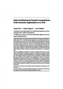
The square-corner partitioning differs from the rectangular partitioning described above by relaxing the restriction that all partitions must be rectangular. Instead we extend the two node partitioning presented in [4] by creating two square partitions in diagonally opposite corners of the matrix. Since the total volume of communication is proportional to the sum of half perimeters of the partitions, it is easy to show that the sum of half perimeters is at a minimum when the two slower nodes are assigned the square partitions. Therefore, the optimal square corner partitioning assigns the balance of the matrix to the fastest node. Since a square has the smallest perimeter of any rectangle of a given area we do not consider nonsquare rectangular corner partitions. Figure 3 shows the partitioning scheme used by the square-corner partitioning and the necessary data movements. The total volume of communication of the squarecorner partitioning is given by (3.4), where X and Y are the areas assigned to nodes 2 and 3 (the two slower nodes). 2× N ×( X + Y )
(3.4)
As Figure 3 shows, nodes 2 and 3 do not communicate at all, thus the total volume of communication is equal to (3.4) for both the fully connected and linear array topology where node 1 is the middle node.
Figure 3. The partitions and data movements of the three node square-corner partitioning. Other similar (but non square-corner) partitioning methods were also investigated. In the square-corner partitioning, diagonally opposite corners are chosen to minimize the number of communication steps necessary. As shown in Figure 3 this number is eight. Placing the squares in corners that are not diagonally opposite requires ten communication steps provided X ≠ Y. If X = Y the number of steps remains at eight. The total volume of communication is still equal to (3.4) regardless. All other partitioning methods investigated resulted in an increased total volume of communication. In the square-corner partitioning, the squares cannot overlap. This imposes the following restriction on the relative speeds of the nodes S2 S3 1 , × ≤ S1 S1 4
(3.5)
where S1+S2+S3=1 and S1 is the relative speed of the node owing the balance of the matrix (the fastest node).
3.1 Comparison of Communications on a Linear Array Topology Since in the square-corner partitioning nodes 2 and 3 do not have to communicate at all, the total volume of communication on a linear array where node 1 is the middle node remains equal to (3.4). The rectangular partitioning has a total volume of communication equal to (3.3). In terms of processor speeds, the squarecorner partitioning has a lower total volume of communication when ( S2 + S3 ) < 1.5 − S1 is satisfied,
where S1:S2:S3 is the ratio representing the node speeds, normalized so that S1+S2+S3=1, and subject to the restriction of (3.5). In order to see when the square-corner partitioning has a lower total volume of communication than the rectangular partitioning, we plotted the surface z = ( S3 + S 2 ) − 1.5 + S1 which represents the rectangular partitioning’s total volume of communication subtracted from that of the squarecorner partitioning. Since for all positive values of S1, S2, and S3, z < 0, the square-corner partitioning always results in a lower total volume of communication. Additionally, the fact that node 1 must now relay data from node 2 to node 3 and vice-versa introduces a section of the communication schedule that is necessarily serialized. The square-corner partitioning has no such section and can therefore exploit in full any existing network parallelism.
3.2 Comparison of Communications of a Fully Connected Topology On a fully connected topology the square-corner partitioning has a total volume of communication equal to (3.4) and the rectangular partitioning has a total volume of communication equal to (3.2). In terms of processor speeds the square-corner partitioning results in a lower total volume of communication when S ( S2 + S3 ) < 1 − 1 is satisfied, where again S1:S2:S3 2 is the ratio representing the node speeds, normalized so that S1+S2+S3=1, and subject to the restriction of (3.5). This inequality shows that the total volume of communication is dependent on the values of S2 and S3 (S1 can be expressed as 1-S2-S3). To investigate what values of S2 and S3 result in a lower total volume of communication compared to the rectangular partitioning, we plotted the surface z = ( S 2 + S3 ) − 1 +
S1 2
(3.9)
which is negative when the square-corner partitionng’s total volume of communication is less than that of the rectangular partitioning. Figure 4 shows a contour plot of this surface at z = 0. The hatched region represents values of S2 and S3 which violate (3.5). The striped region has values of z < 0, and therefore in this region the total volume of communication for the squarecorner partitioning is less than that of the rectangular partitioning. The white region has values of z > 0 indicating that the square-corner partitioning has a total volume of communication greater than that of the rectangular partitioning.
Figure 5. A rectangular partitioning for three nodes.
Figure 4. A contour plot of the surface represented by (3.9) at z = 0.
3.3 Comparison with state-of-the-art and the Lower Bound In section 2 we summarized the work in [3]. The authors present an algorithm to find an optimal rectangular partitioning with the restriction that the rectangles are arranged in columns. For three nodes, this algorithm results in a partitioning similar to Figure 5, with three rectangles proportional in area to the relative powers of the nodes. The sum of halfperimeters s which is proportional to the total volume of communication was given by (2.1), and in the case p of three nodes, is equal to ∑ i=1 ( hi + wi ) = 3 × N + q , where 0 < q < N. The lower bound of the sum of half perimeters l is given by (2.2), and for the case of three nodes l = 2 × ∑ i =1 ai = 2 × ( a1 + a2 + a3 ) where ai is the p
area of the partition belonging to node i. In the case of three nodes, the square-corner partitioning has a sum of half perimeters s = 2 × ( N + X + Y ) . This equation shows that for the square-corner partitioning, as X , Y → 0, s → 2 N , which is equal to the lower bound that cannot be met by the rectangular partitioning. To compare the square-corner sum of halfperimeters with that of the rectangular partitioning and the lower bound, we adopted the same approach as in [3]. We generated 2,000,000 random values for the partition areas a1 = N2-X-Y, a2 = X, and a3 = Y, and calculated values for the sum of half-perimeters s and the lower bound l. Since we already know that the total volume of communication for the square-corner partitioning (on a fully connected network) is greater for the cases where (3.9) is positive, we restrict the random areas a1, a2, and a3 accordingly.
The average sum of half-perimeter to lower bound ratio for the rectangular partitioning is 1.128, while that of the square-corner partitioning is 1.079. Considering that 1.0 is the optimum value, this is an improvement of 38%. The minimum value for the sum of half-perimeter to lower bound ratio for the rectangular partitioning is 1.0595, while that of the square-corner partitioning is 1.0001, an improvement of well over 99%. This also shows that the squarecorner partitioning does approach the lower bound which cannot be met by the rectangular partitioning. In generating 2,000,000 random areas, there are bound to be many that are have very large ratios, making them computationally unrealistic. Surely nobody would use two nodes in parallel if one of them is slower than the other by an order of hundreds or thousands or greater. We therefore imposed the tighter but more realistic restriction of amax / amin ≤ 100 . Even with these much tighter restrictions, the average sum of half-perimeter to lower bound ratio for the rectangular partitioning is 1.104 while that of square-corner partitioning is 1.062, an improvement of 40%. The minimum is improved from 1.059 to 1.008, an improvement of 86%.
3.4 Overlapping Computations and Communications The other primary benefit of the square-corner partitioning is overlapping communications and computations. As seen in Figure 3, and in more detail Figure 6, there is a sub-partition C1 of node 1’s C partition which is immediately calculable – no communications are necessary to compute the product of this sub-partition. On an architecture which has a dedicated communications sub-system this quality can be exploited to overlap some communications and computations.
Figure 6. The shaded areas represent node 1’s partition. The sub-partition C1=A1xB1 is immediately calculable – no communications are necessary to compute its product. Figure 7 shows a schematic of the overlapping of communication and computation from an execution time point of view. As the areas C2, X, and Y (in Figure 6) are calculated to be proportional to the speed of the nodes owning them, it is expected that steps III, IV, and V will finish their computations at the same time. The same is not true for steps I and II, as they represent unrelated tasks.
The ratio of speeds between the three nodes were varied by slowing down CPUs when required using a CPU limiting program as proposed in [5]. This program supervises a specified processes and using the /proc pseudo-filesystem, forces the process to sleep when it has used more than a specified fraction of CPU time. The process is then woken when enough idle CPU time has elapsed for the process to resume. Sampled frequently enough, this provides a fine level of control over the CPU speed. Comparison of the runtimes of each node confirmed that this method results in the desired ratios to within 2%. For simplicity we present results where the speeds of the slower nodes (S2 and S3) equal. We varied this relative value from 5 to 25, where S1 = 100 - S2 - S3. Network bandwidth is 100Mb/s, and N = 5000. Figure 8 shows the communication times for the square-corner and rectangular partitionings on the linear array topology. The square-corner has a lower communication time than the rectangular linear array in all cases. On average the square-corner partitioning results in a reduction in communication time of 40%.
Figure 7. Overlapping Communication and Computation from an execution-time point of view. A solution exists which would minimize the overall execution time but this would alter the approach of the square-corner partitioning. Thus we formulate the total execution time as texe = max(I,II) + max(III,IV,V) .
4. Experimental Results To experimentally verify this new partitioning, we implemented matrix multiplications utilizing the optimal square-corner partitioning and the optimal rectangular partitioning in Open-MPI [7]. Local matrix multiplications utilize ATLAS [10]. Experiments were carried out on three identical machines to eliminate contributions of architectural differences. The machines were connected with a full duplex Ethernet switch that allows the bandwidth between the nodes to be finely controlled.
Figure 8. Communication times for the square-corner and rectangular partitionings on the linear array topology. Relative speeds S1+S2+S3 = 100. A plot of the communication volumes agrees well with Figure 8 with one exception. The rectangular and square-corner communication volumes converge as S2,S3→25. The reason that the communication times do not converge is due to the necessarily sequential component of the rectangular partitioning’s communication schedule. This component can not make use of network parallelism such as Ethernet’s full
duplex. Experiments “illegally” altering the rectangular partitioning’s communication schedule (by deserializing necessarily serial communications) confirm this. Figure 9 shows a plot of the execution times for the square-corner and rectangular partitionings on the linear array topology. For the square-corner partitioning two values are plotted, the execution time obtained with no overlapping of communication and computation, and the values obtained with overlapping. It is seen that with no overlapping (only taking into account the communication differences) the execution time for the square-corner partitioning is on average 14% less than that of the rectangular, and that the reduction in communication times seen in Figure 8 directly influence the execution times.
reason for this is that the total volume of communication for this partitioning increases much slower than that of both the rectangular partitioning on the linear array and the square-corner partitioning. It increases so much slower that the increased benefit of more computational parallelism (as S2 and S3 get closer to S1) outweighs the higher communication burden. Still, for ratios more heterogeneous than about 80:10:10, the square-corner partitioning has a lower total volume of communication, and therefore lower communication times.
Figure 10. Communication times for the square-corner and rectangular partitionings on a fully connected topology. Relative speeds S1+S2+S3 = 100.
Figure 9. Execution times for the square-corner and rectangular partitionings on the linear array topology. Relative speeds S1+S2+S3 = 100. The introduction of overlapping communication and communications significantly influences the performance of the square-corner partitioning. For a ratio of 90:5:5 it is 38% faster than the rectangular partitioning. As the ratio approaches 50:25:25, the amount of overlap possible tends to zero, and the execution times of the square-corner partitioning with and without overlap converge. Figure 10 shows the Communication times for the fully connected topology. A notable aspect is that the rectangular partitioning’s communication times decrease despite the fact that it is dealing with increasingly higher communication volumes. The
Figure 11 shows the overall execution times for the square-corner and rectangular partitionings on a fully connected topology. Again the square-corner partitioning is shown with and without overlapping. Again, without overlapping the execution times are directly affected by the communication times. For ratios more heterogeneous than about 80:10:10, the square-corner partitioning outperforms the rectangular. The introduction of overlapping again significantly influences the performance of the square-corner partitioning. For a ratio of 90:5:5 the square-corner partitioning is 30% faster that the rectangular. Additionally, the range of ratios where the squarecorner is faster than the rectangular is broadened from about 80:10:10 to about 60:20:20. Similar results were seen at other bandwidths, values of N, and power ratios, including where S2 ≠ S3.
We determine that this partitioning is viable and future work will include employing it as the top-level partitioning of a hierarchal algorithm that will perform parallel computations across three interconnected clusters. This work was supported by Science Foundation Ireland.
References [1] Jorge G. Barbosa, João Tavares and Armando J. Padilha, “Linear Algebra Algorithms in a Heterogeneous Cluster of th Personal Computers”, Proceedings of the 9 Heterogeneous Computing Workshop (HCW 2000), 2000
Figure 11. Execution times for the square-corner and rectangular partitionings on a fully connected topology. Relative speeds S1+S2+S3 = 100.
5. Conclusion We presented a new ‘square-corner’ data partitioning strategy for parallel computing on three interconnected clusters. This partitioning has two advantages over existing partitionings. First it reduces communication time due to a lower total volume of communication and a more efficient communication schedule. The total volume of communication is shown to approach the known lower bound unlike existing partitionings. Second it allows for the overlapping of communication and computation. To determine the viability of this partitioning we modeled the three cluster topology with three processors performing matrix multiplications. Compared to more general partitionings which result in simple ‘rectangular’ partitions the square-corner partitioning is shown to reduce the total volume of communication in all cases for the linear array topology and in most cases for a fully connected topology. We experimentally show that this directly translates to lower communication times. In the case of the linear array topology, we show average reductions in communication time of about 40%. Further experimentation shows that this reduction in communication time directly translates to a reduction in the overall execution time, aided by a more efficient communication schedule. Overlapping communication and computation brings further benefit, in both reducing the execution times significantly, and broadening the ratio range where the square-corner partitioning outperforms the rectangular partitioning on a fully connected topology. MPI experiments demonstrate reductions in execution times of up to 38%.
[2] Olivier Beaumont, Vincent Boudet, Fabrice Rastello and Yves Robert, “Partitioning a Square into Rectangles: NPCompleteness and Approximation Algorithms”, Algorithmica, 2002, Vol.34, No.3, pp.217-239 [3] Olivier Beaumont, Vincent Boudet, Fabrice Rastello and Yves Robert, “Matrix-Matrix Multiplication on Heterogeneous Platforms”, IEEE Transactions on Parallel and Distributed Systems, 2001, Vol.12, No.10, pp.1033-1051 [4] Brett A. Becker and Alexey Lastovetsky, “Matrix Multiplication on Two Interconnected Processors”, Proceedings of the 8th IEEE International Conference on Cluster Computing (Cluster 2006), 2006. [5] Louis-Claude Canon and Emmanuel Jeannot, “Wrekavoc: a Tool for Emulating Heterogeneity”, Proceedings of the International Parallel and Distributed Processing Symposium (IPDPS 2006), 2006. [6] Egor Dovolnov, Alexey Kalinov and Sergey Klimov, “Natural Block Data Decomposition for Heterogeneous th Clusters”, Proceedings of the 17 International Parallel and Distributed Processing Symposium (IPDPS 2003), 2003 [7] Edgar Gabriel et. al., “Open MPI: Goals, Concept, and Design of a Next Generation MPI Implementation”, Proceedings of the 11th European PVM/MPI Users' Group Meeting,(Euro PVM/MPI 2004) 2004 [8] The Jabberwocky Project, http://jabberwocky.anu.edu.au/ [9] Alexey Kalinov and Alexey Lastovetsky, "Heterogeneous Distribution of Computations While Solving Linear Algebra Problems on Networks of Heterogeneous Computers", Proceedings of the 7th International Conference on High Performance Computing and Networking Europe (HPCN`99), 1999. [10] R. Clint Whaley and Jack Dongarra, “Automatically Tuned Linear Algebra Software”, Ninth SIAM Conference on Parallel Processing for Scientific Computing, 1999.