AbstractâThis paper describes a set of TDMA MAC protocols for wireless sensor ... data gathering for disaster recovery and tracking rapid move- ment through a ...
Towards Optimal TDMA Frame Size in Wireless Sensor Networks Kevin L. Bryan, Tiegeng Ren, Lisa DiPippo, Timothy Henry, Victor Fay-Wolfe {bryank,rentg,dipippo,tmh,wolfe}@cs.uri.edu University of Rhode Island, Kingston, RI 02881
Abstract—This paper describes a set of TDMA MAC protocols for wireless sensor networks that can achieve near-optimal throughput and good latency for regular periodic data delivery. The protocol is based on a novel graph coloring technique called the Color Constraint Heuristic (CCH) The paper describes a centralized TDMA slot assignment algorithm, Centralized Slot Assignment (CSA-CCH), that uses CCH. It then describes a distributed version of the algorithm, Distributed Slot Assignment (DSA-CCH. A further refinement of DSA that is designed for query tree aggregation applications (DSA-AGGR) is also presented. The paper shows through simulations that our algorithm performs closer to the optimal bound on data throughput than several prominent TDMA slot assignment protocols for wireless sensor networks. In addition, the CCH-based algorithms carefully order the coloring to provide good latency for data delivery.
I. I NTRODUCTION Wireless Sensor Networks (WSN) are becoming popular as solutions to an increasing number of application areas. Monitoring the stress and pressure on a building’s framework, data gathering for disaster recovery and tracking rapid movement through a sensor field all require high query rates and consistent, timely delivery of data in order to ensure that data’s usefulness. Contention based MACs behave quite poorly under these circumstances[1] and are not acceptable in real-time or time-sensitive applications. Time-division multiple access (TDMA) scheduling can eliminate collisions and remove the need for a backoff. This increased predictability can better meet the requirements for high query rate and timely data delivery in high traffic scenarios. Applications like those described above may require data to be collected at the nodes and aggregated up to a base station. It may also require that information, like code updates, be flooded throughout the network to quickly reset the state of the nodes. These applications have specific requirements that we articulate here in a list of criteria. We will use these criteria to evaluate the MAC protocols that we have developed. • Predictability: When a node in the sensor network detects that a critical value has changed, there must be a level of certainty that the data will be received by the base station within a specified time, and that the data is still valid. • Timeliness: Along with being predictable, the delivery of data in these types of applications must also be fast. Thus, the latency of data delivery should be minimized. Further, if periodic requests are made for data delivery
from the sensor network, the rate at which the query results are returned should be maximized, thus increasing overall throughput of the application. • Power efficiency: Many sensor networks are made up of wireless nodes that run on limited battery power. Protocol development must consider the energy cost of a successful message transmission. It must also consider how much energy must be expended before the network can perform useful data transmission (set-up cost). • Adaptability: The sensor network should be able to adapt to nodes entering and leaving the network. This may come from design, in networks with mobile nodes, or it may come from node failure during the lifetime of the network. • Scalability: Sensor network protocol solutions should work for small networks as well as larger networks without incurring a large increase in cost in terms of power, timeliness, adaptability, and predictability. Scalability can be viewed in terms of number of nodes in the network as well as density of the nodes in the network. The benefit of having a conflict-free TDMA schedule is clear: as the number of collisions is reduced or eliminated, the throughput of the network can be greatly improved by the corresponding reduction in retransmits. For flooding applications, this means data can be disseminated a great deal faster. For applications in which data is aggregated from sensors to a base station, these improvements imply the possibility of quicker rates for receipt of periodic data collection. Recently, there has been research into applying graph coloring theory to the assignment of time slots in a TDMA schedule [2], [3], [4]. One of the goals of this work is to reduce the number of colors used, and thus reduce the number of time slots necessary for the schedule. We have developed a set of TDMA-based MAC protocols based on coloring graphs Our algorithms provide near-optimal slot assignment using a heuristic that carefully addresses the order of coloring. We first describe a centralized protocol, Centralized Slot Assignment (CSA-CCH) that assumes knowledge of the entire network topology. We then describe a distributed version of the algorithm, Distributed Slot Assignment (DSA-CCH) that does not assume any prior knowledge of the network, and thus could be used in any real sensor network deployment. The rest of this paper is organized as follows. Section II provides a discussion of the mapping of the graph coloring
2
χ ∆ G2 ∆(G2 ) clique ω
Minimum number of colors to color a graph Maximum degree of any vertex in a graph The square of graph G The maximum degree of G2 A fully connected neighborhood of nodes Maximum clique size in a graph TABLE I G RAPH N OTATION Fig. 1.
problem to the assignment of slots in a WSN TDMA protocol. Section III presents related work in WSN TDMA slot assignment using both centralized and distributed algorithms. Section IV describes our algorithms. Section V presents a set of simulations that we conducted to compare our algorithms with existing graph-coloring TDMA algorithms. Finally, Section VI summarizes our important results, and discusses future work. II. WSN AND G RAPH C OLORING Graph coloring theory can be applied to frequency or time slot assignment in wireless sensor networks. In this section we provide background in the applicable graph theory, discuss how it can be mapped to the WSN slot assignment problem, and describe the network model that we have chosen to follow in our work. A. Graph Coloring Graph coloring is a classic problem in graph theory. The idea is to color/label/number all of the vertices of a graph such that adjacent nodes never have the same color. The smallest number of colors that can be used to color a graph G is the chromatic number of G and is denoted χ(G). When it is clear from context, we will just use χ. There is a large body of research on the chromatic number of graphs. The computational complexity of finding the optimal solution is proven to be NP-hard and χ is bounded by ω ≤ χ ≤ ∆ + 1 [5], where ω is the maximum clique size in the graph, and ∆ is the maximum degree of any vertex of the graph, (see Table I for a summary of notation). For any greedy coloring algorithm, the worst case number of colors is ∆ + 1. A generalization of graph coloring may contain more constraints. One such generalization is the L(p, q)-labeling where the labels of neighboring vertices differ by at least p and the labels of vertices at distance two differ by at least q [6]. The L(p, q)-labeling problem has been studied well in the past, as summarized by Bodlaender et. al in [7]. The L(1, 1)-labeling problem, is also known as the distance2 coloring problem [8]. It is equivalent to the coloring of the square of a graph that has been stated in [9]. The square of a graph G is the graph G2 such that the edge (u, v) is in G2 if and only if there is a distance of at most two edges between the u and v. The order in which colors are assigned to nodes can dramatically affect the number of colors used. Sorting vertices by decreasing degree is an ordering heuristic suggested in [5] that reduces the number of colors in a graph.
Square of UD graph
B. Mapping to WSN There are two types of potential communication collisions in a wireless sensor network using TDMA. The first is direct collision, in which any pair of neighbor transmitters are assigned the same time slot. This prevents each from hearing anything sent from the other since they transmit simultaneously. The second is a hidden collision, in which a node cannot hear anything during a listening slot if two of its neighbors are assigned to transmit during that same time slot and therefore transmit at the same time. In the radio literature this is referred to as the hidden terminal problem. When coloring a graph for WSN scheduling both types of collisions must be considered. To model TDMA slot assignments in terms of the graph theory coloring problem, we map nodes to vertices in the graph, and links to edges. Each color represents a TDMA time slot. We consider L(1, 1)-labeling (coloring the square of the graph) because the square of the graph consists of the graph containing the two-hop neighborhoods for all nodes, and thus avoid both direct and hidden collisions. The fewer colors needed for the graph, the fewer time slots and smaller resulting frame size. For applications in which data is flooded throughout the network, a smaller frame size will reduce latency in distributing the data since a greater amount of data can be transmitted in a fixed amount of time. In applications that rely on data aggregation, the query rate can be increased with a smaller frame size. A data query rate as high as max 1color can be achieved by any conflict-free schedule. This is easy to see by considering some node n. If n’s slot is t, then in the max color slots before t, all of n’s neighbors have been able to send data, which must include transmissions from all of n’s children. Thus, n can aggregate it’s children’s data with its own data for transmission at time t. C. Unit Disk Radio Model A Unit Disk Graph (UD) [10], [11] can be used to model a sensor network because the radius of the disk can be considered the transmission distance for the radios on the nodes. Thus, two nodes are considered adjacent if the first node is within the radius of a unit disk centered at the second node. We extend this concept further to consider the square of the UD graph. This represents the two-hop neighborhoods of the nodes in the network. Figure 1 depicts the square of a UD graph. There are four disks of diameter one centered by vertices {u, v, w, x}. If the center of a disk is under the coverage of another disk, there’s an edge between the centers of these two disks in the UD
3
graph G. For example, in the diagram v and u are neighbors, as are w and u. Solid lines indicate an edge in graph G. G(V, E) = G({u, v, w, x}, {{uv}, {uw}}) In the square of the graph G, G2 , there is an edge between v and w (the dashed line), since v and w are distance two in G. G2 (V, E) = G({u, v, w, x}, {{uv}, {uw}, {vw}}) In previous work, we have proven an upper bound on the chromatic number for G2 of a UDG that is linear with respect to ω(G) for these graphs [12]. III. R ELATED W ORK Recently there has been a large amount of research done in the area of MAC protocols for wireless sensor networks. In this section, we describe some of the general results in this area, as well as results of applying graph coloring theory to WSN MAC protocols. Langendoen and Halkes [13] present a recent survey of MAC protocols for WSNs. They describe CSMA and TDMA protocols, and compare them based on various criteria. The authors mention the power benefit of using TDMA protocols because nodes can turn off their radios when they are not scheduled to send or receive. While some MAC protocols that use TDMA strategies allow for some collisions [14], [15], all of the graph coloring MAC protocols that we consider generate conflict free schedules. As noted in [2], there are drawbacks and challenges to TDMA scheduling for WSN’s in terms of clock drifting, flexibility and the ability to adapt to interference from nodes not considered as neighbors. However, there are various solutions to these issues. Clock drifting can be handled by a buffer at the beginning of a slot (other proposals to deal with clock drifting appear in [16]). Topological flexibility can be introduced by having nodes recolor at random intervals. A major distinction among the various graph coloring based algorithms that we examine is where the coloring decision is made. In some of the algorithms (centralized), it is assumed there is a single entity that has full knowledge of the network topology. This is consistent in an environment where the nodes are systematically placed and the queries and data sink are stable. Distributed algorithms remove these strong assumptions and instead allow the nodes to color themselves. In most cases, we would expect better performance from a centralized algorithm, as it has more information with which to work. However, some centralized algorithms, such as RAND [17], do not make use of a priori information. Distributed algorithms are applicable on a wider variety of applications when centralized knowledge of topology is not possible. A. Centralized In [17] the authors discuss three breadth-first centralized algorithms which vary the labeling order of the nodes. The first approach is called RAND whereby any node in the uncolored list is chosen at random to be the next node assigned a color. The Minimum Neighborhood First (MNF) labels nodes from
those having few neighbors to those with many neighbors. The nodes are then colored in reverse order of their labeling. The Progressive Minimum Neighborhood First (PMNF) is similar to MNF, but once a node has been labeled, that node and the corresponding connections are removed from the graph. Therefore, the neighborhoods consistently change during the labeling and must be recalculated with each step. The MNF and PMNF algorithms cannot be distributed because their ordering requires global information. The authors state the worst case coloring could be as high as the maximum distance2 neighborhood in the graph, ∆(G2 ). qMAC [4] is a protocol in which coloring begins at the data sink and proceeds breadth-first (referred to here as BF). A token containing the current coloring is passed amongst the uncolored nodes. When a node receives the token, it colors itself with the lowest available color that will not cause conflicts. Because the token builds a map of the global structure, a distributed version of this protocol is possible, but it must still retain its sequential nature for color assignments. There’s another centralized algorithm for coloring a graph The Degree Heuristic (DH) is a centralized greedy algorithm that colors the nodes in the graph in order of nodes’ degree from highest to lowest [5]. The work in [18] provides a First-Fit algorithm that leads to a low bound very close to optimal for L(1, 1)-Labeling for Disk Graphs by utilizing the geometric properties of unit disk graphs. However, there’s no implementation of this technique in wireless sensor network, and it is not translatable to a distributed solution. B. Distributed DRAND [2] is a distributed version of RAND. Each node chooses its own color on a random schedule, and refreshes the color periodically. In order to prevent nodes that are separated by two hops from attempting to assign their colors at the same time, it uses a locking scheme where the node requests a lock from each of the one hop neighbors before setting its color. If granted, those neighbors will deny requests from other nodes in their one hop neighborhood (the original node’s two hop neighborhood) until the color is assigned and the lock is released. This allows DRAND to complete its initial coloring within a time proportional to ∆(G2 ). DRAND randomizes the order of the nodes to be colored. While this allows for parallelism in setup, it does not allow the protocol to choose the order in which the nodes are colored. Thus, in the worst case DRAND performs like a greedy algorithm which uses ∆(G2 ) colors. In [4], the authors do not provide a distributed solution for qMAC. Instead they recommend using the distributed coloring algorithm of DRAND or the one found in [19] which implements a distributed breadth-first search in sensor networks. However, this solution has drawbacks. First, it has a performance issue based on the token passing. That is, the algorithm would be O(n) in number of nodes, since it could not implement parallelism in the coloring. Also, the bookkeeping for a breadth-first search would create significant
4
overhead since each node must request and pass a token containing the developing tree structure. Work by [20] provides two distributed algorithms for Distance − 2 coloring in Unit Disk Graphs. However, their goal is on shorter setup time for a conflict-free schedule instead of a smaller TDMA frame size. The work in [3] presents DCQS (Dynamic Conflict-free Query Scheduling) a TDMA protocol designed specifically for query services with in-network data aggregation. It exploits the precedence constraints imposed by the query path and data aggregation. This solution assigns TDMA slots based on these precedence constraints, and unlike our work, their algorithms use edge coloring, instead of node coloring. Our work seeks to improve on current protocol algorithms in two key ways: reducing the number of colors and thereby the frame size and intelligently ordering colors to reduce the latency caused by “color-inversions” on the path to a base station. IV. A LGORITHMS Our goal in developing MAC protocols is to find a coloring for the TDMA schedule, such that the TDMA frame size is as low as possible to reduces latency and maximize the level of certainty that data will be received within a specified time. This translates into a coloring that approaches the minimum achievable number of colors and has small positive color distances along data paths. The color distance of two nodes is the difference between the numerical representations (slots) of their colors. In a data aggregation application, a positive color distance indicates that a parent node will have received data from its child node along the data path prior to its own transmission slot time. A. Color Constraint Heuristic (CCH) Randomized slot assignment algorithms, such as RAND and DRAND, lose the advantage that can be gained from a careful ordering of the node colors or slots and can approach ∆(G2 )[2] in number of colors. We have developed a lightweight and efficient heuristic, the Color Constraint Heuristic (CCH), for choosing the order in which to color nodes in a graph. If we always color the most constrained node in the entire network, we arrive at a very efficient order for coloring the network. The “most-constrained” node is the node whose number of already colored neighbors gives it the least freedom in selecting a color for itself. To determine the most constrained node, we use a weighted sum of the one hop and two hop neighbors that have been previously colored. A higher weight is given to one hop neighbors, as they more directly affect the color choices. CCH Ordering = 2 · ColoredOneHop + ColoredT woHop
When choosing a node to be colored, we pick the node with the highest value of CCH Ordering. Once a node has been selected for coloring, it is colored with the lowest available color in its two-hop neighborhood.
B. Centralized CCH Slot Assignment (CSA-CCH) A centralized coloring algorithm must make color decisions for individual nodes based on an overview of the entire graph. For example, a centralized greedy coloring of a graph will order the vertices by decreasing degree and then color the nodes in that order. This can lead to fewer number of colors for most graphs, however, in the worst case, it would lead to ∆(G) + 1 as other greedy algorithm does. For our centralized CSA-CCH algorithm, we start at the base station, if one exists, or the highest degree node in the original graph, and then spread the coloring decisions out from that node. While this could be performed in a strict breadth first pattern, we use the highest CCH value among uncolored nodes as an indicator of which node to color. The CCH is then re-computed for nodes neighboring the colored node. C. Distributed CCH Slot Assignment (DSA-CCH) In our distributed algorithm (DSA), a spreading scheme can be used to color nodes. The coloring starts at one point (e.g. base station) and all its one hop neighbors, then each node must wait until a sufficient number of its neighbors are colored before it can color itself. To determine how many neighbors must be colored prior to a node coloring itself, we use the ratio of a weighted sum of the one hop and two hop neighborhood sizes to a weighted sum of the one hop and two hop neighbors that have been previously colored. color score =
2 · ColoredOneHop + ColoredT woHop 2 · N umberOneHops + N umberT woHops
In our distributed DSA-CCH algorithm, it would be extremely expensive to do global scoring. Instead, we use a “coloring threshold”, a percentage of already colored neighbors in a node’s two-hop neighborhood. For our preliminary tests, we used 0.25 for the color score threshold. Therefore, a node will color itself if its color score is greater than 0.25. This is performed in a distributed manner so that each node can start to color itself based on its own environment. The color score provides a means to balance the coloring between breadthfirst and depth-first. The 0.25 used in these simulations was selected so that the ordering is weighted towards a breadthfirst. While the 0.25 color score threshold works well in many cases, it is possible that for some topologies the coloring cannot propagate through the entire network. For example, when a single node is bridging two larger networks. Edge nodes in the second neighborhood will never have a color score high enough to self-color. This is an area for future work and possible solutions to this will be discussed in Section VI. The distributed DSA-CCH algorithm uses the node locking mechanism of DRAND to avoid deadlock and ensure consistency. Our approach comes at the cost of scalability because it is a spreading approach, rather than the extremely parallel color assignments of which DRAND is capable. Parallelism in DSA-CCH increases as the boundary between colored and uncolored nodes increases. In networks that are used for data
5
f u n c t i o n ReadyToColor : i f 2 ∗ ( ColoredOneHop ) + ( ColoredTwoHop ) / ( 2 ∗ NumberOneHops ) + NumberTwoHops ) ) > 0.25: return True return False f u n c t i o n ChooseColor ( c o l o r T a b l e ) : parentcolor = colorTable [ parent ] # P r e f e r c o l o r j u s t below p a r e n t ’ s c o l o r f o r n e x t c o l o r : = p a r e n t c o l o r − 1 downto 0 : i f n e x t c o l o r not in c o l o r T a b l e : return n e x t c o l o r # I f no s u c h c o l o r i s f o u n d above , # t h e n p i c k a c o l o r n e a r t h e end # of th e c u r r e n t high frame s i z e m a x c o l o r = max ( max ( c o l o r T a b l e ) , NumberOneHops + 1 ) f o r n e x t c o l o r : = m a x c o l o r − 1 downto p a r e n t c o l o r + 1 : i f n e x t c o l o r not in c o l o r T a b l e : return n e x t c o l o r # I f we do n o t h a v e a c o l o r , c r e a t e a new c o l o r return maxcolor + 1 f u n c t i o n Color : i f RequestLock ( / ∗ [ out ] ∗ / c o l o r T a b l e ) : i f ReadyToColor ( ) : ChooseColor ( c o l o r T a b l e ) ReleaseLock ( )
Fig. 2.
Pseudo-code for DSA-AGGR
aggregation, the coloring time is proportional to the height of the routing tree and node density (in terms of neighborhood size). D. Distributed CCH for Data Aggregation (DSA-AGGR) Data aggregation queries are a common use for sensor networks. We have developed a version of our DSA-CCH algorithm, called DSA-AGGR, that is optimized for coloring aggregation trees. In order to reduce query latency as aggregate values are returned to a base station, we must reduce the number of times a parent’s color number is less than any of it’s children. Each “color inversion” corresponds to an additional frame in the delivery of data to the base station. Our modification to DSA-CCH uses routing tree information in coloring nodes so that there are fewer color inversions, thereby reducing latency. Figure 2 shows the DSA-AGGR algorithm. Not shown there is that the base station starts by coloring itself and its one-hop neighbors (a single transmission with all or most of the one-hop neighbors assigned colors can accomplish this). Note that RequestLock and ReleaseLock work in the same way as in DRAND. Our algorithm ensures that a parent node has a higher numbered slot than its children without introducing any more colors unless absolutely necessary. To do this, we first search for a free slot below the parent’s number. If none is found, then we start from either the maximum color in the two hop neighborhood or the nodes degree, whichever is higher. In trial runs, there was a negligible difference in the number of colors DSA-AGGR used compared to DSA-CCH. However, DSA-AGGR has significantly improved performance on an aggregation query and maintains performance similar to DSACCH in flooding distributions. Details of this are shown in Section V.
V. S IMULATIONS In order to evaluate how well our algorithms meet the criteria specified in Section I, we performed a series of tests comparing them to similar protocols. In the first test, the Node Coloring Test, we measured how many colors, or TDMA slots, are used by the various algorithms. This gives an indication of how close our algorithm is to the optimal coloring. We next performed a Startup Cost test to measured the energy and time need to compute the slot assignments for each of the distributed TDMA protocols. The third test (Data Flooding) demonstrates the performance of the TDMA algorithm in an application that has each node sending data to every other node. This represents a high traffic scenario in which the throughput of the nodes is critical. The final test, for Data Aggregation, evaluates the performance of our algorithms, and others, in a query routing scenario. Data is collected at sensor nodes, and is routed and aggregated up a tree to the base station. The protocols we compare with our CSA and DSA are RAND, DRAND, DH, and BF. DH and BF are selected because they are recognized as efficient centralized coloring schemes in graph theory. We want to compare them with ours to show how our choice of CCH for ordering the nodes to color is valid. Since there these coloring schemes have no WSN MAC protocol developed that we know of, and they don’t lend themselves to distributed solutions, we do not apply them in our other simulations. All of our tests were run on our own URIMACSim simulator which is designed specifically for testing TDMA-based algorithms over hundreds of nodes. The simulator runs a fixedclock where each node is processed for each TDMA slot. The state of each node can be one of: sleep, idle, transmit, receive or collision. In each slot the simulator determines the state of a node based on the predetermined slot assignments. If the node is assigned a slot for transmission, its state is set to transmit. If one of the node’s neighbors is assigned to transmit in the slot, its state is set to receive. If more than one of the node’s neighbors is assigned to transmit in the slot, its state is set to collision. In any other case, the node’s state is set to either idle or to sleep (if the algorithm allows sleeping). Collisions are treated the same as receives with respect to power consumption. While this simplification reduces the usefulness of the simulator for several important metrics, we believe the numbers obtained provide a reasonable guideline for use in designing algorithms that can be tested in a more complete simulator at a later time. A. Simulation Metrics The specific measurements that we used in the four tests that we performed are described here. • Frame Size: number of colors/slots used. • Extra Colors: number of colors used above the optimal number. • Startup Time: amount of time used to color all of the nodes in the network.
6
Startup Energy Cost: energy is used to perform the node coloring at startup. • Completion over time: percentage of nodes receiving all data from other nodes in the network over time. • Max Latency: time from when a sensor is read until that data is aggregated at the base station. Each of the simulations was run on two different topologies within a fixed dimension box of 100 × 100 units. The first 100 100 topology places each mote randomly in a sqrt(N ) by sqrt(N ) box within a regular grid and N ranging from 81 to 400 (thus, effectively increasing the density). The second topology places nodes randomly throughout the 100 × 100 space. These two topologies will be referred to as Grid-Random and Random respectively. In both scenarios, the communication radius was fixed at 20 units. Tests were run with the same set of PRNG seeds so that identical topologies would be run by each of the algorithms. •
180
∆(G) DH BF CSA DSA RAND 140 DRAND 2 ∆(G ) 120 Frame Size
160
100
80
60
40
20
0 50
100
150
200
250
300
350
400
350
400
Number of Nodes
(a) Frame on Grid-Random topology 35 CSA DH BF DSA RAND DRAND
30
25
20
15
10
5
0 50
100
150
200
250
300
Number of Nodes
(b) Extra colors used on Grid-Random topology 200
∆(G) DH BF CSA DSA 160 RAND DRAND ∆(G2) 140 180
Frame Size
120 100 80 60 40 20 0 50
100
150
200
250
300
350
400
350
400
Number of Nodes
(c) Frame size on Random topology 25 CSA DH BF DSA RAND 20 DRAND
Extra Colors
The first set of simulations examined the number of colors used by each algorithm. Each topology/algorithm pair was run ten times and the data was averaged. Figure 3(a) shows that DSA-CCH uses 12% to 21% fewer colors than DRAND with an average savings of 17.6% over all densities. Our centralized algorithm CSA-CCH requires 22.9% fewer colors than the corresponding centralized RAND algorithm. Notice that this figure and Figure 3(c) show the upper and lower bounds on the number of colors, ∆(G2 ) and ∆(G) respectively, since both are served as base line test in literatures frequently. Figures 3(b) and 3(d) show the performance of each algorithm compared to the lower bound of colors needed (∆(G)) by illustrating how many extra colors each algorithm uses over the number used by the optimal coloring. Figure 3(b) and 3(d) also shows that CSA performs better than DH and BF in all topologies (2.5% better than DH and 4.5% than BF in Random topology; 1.1% better than DH and 4% than BF in Grid-Random topology). This validates our CCH as a good choice for ordering node coloring. CSA performs slightly better than the well-established node coloring heuristics, DH and BF, and it has a distributed solution that is more realistic in most WSN applications. Figures 3(c) and 3(d), show that our CCH-based algorithms perform slightly better than RAND and DRAND on a Random topology. This variance allows all coloring algorithms to frequently reuse lower numbers instead of adding an extra color. However, such varied node density itself does not guarantee that the chromatic number (of G2 ) is less. We consider the effect of layout on this bound to be future work.
Extra Colors
B. Node Coloring Test
15
10
5
C. Startup Cost Test In this test we measured the amount of time and energy that is used in the startup phase of the TDMA protocols. This startup phase involves assigning time slots to each node in the network. Because the centralized protocols assume that all setup is done by some entity that has knowledge of the entire network, we can assume that this is done a priori on a
0 50
100
150
200
250
300
Number of Nodes
(d) Extra colors used on Random topology Fig. 3.
Frame Size Tests
7
45 DSA DRAND 40
35
Setup time
30
20
10
5
0 50
100
150
200
250
300
350
400
Number of nodes
(a) Startup Time Varying over Number of Nodes 35 DSA DRAND 30
Setup time
25
20
15
10
5
0 12
14
16
18
20
22
24
26
28
Nodes density
(b) Startup Time Varying over Network Density 35000 DSA DRAND 30000
25000
20000
15000
10000
5000
0 50
100
150
200
250
300
350
400
Number of nodes
(c) Startup Energy Cost Varying over Number of Nodes
D. Data Flooding Test
40000 DSA DRAND 35000
30000
25000 Energy cost
In the data flooding simulation test, we used a trivial routing strategy where every node in the network floods its message in an attempt to reach every other node. Two observations can be made about this strategy. First, this strategy will only complete in a connected topology. Second, on connected topologies with a no-conflict schedule, the entire flooding will complete. This test can show data dissemination rates when specific data paths are not known. Because the algorithms tested in this set have no routing information, none are biased towards a particular type of dissemination. Figures 5(a) and 5(b), show the number of nodes that have received 100% of the data in each test. The test shows how a shorter frame size helps data move quicker in an all-to-all data flooding scenario, averaging out all possible paths that data could take through the network. By observing
25
15
Energy cost
base station that is not power constrained. Therefore, we only ran this test on the distributed protocols, DSA and DRAND. An important thing to note is that the startup phase for these algorithms must use CSMA for the MAC protocol because the TDMA schedule has not been setup yet. While we modeled most aspects of CSMA in our simulator, it does not completely simulate the performance of CSMA. Thus, the results in these tests do not necessarily reflect a real scenario. However, since the setup for all of the protocols is simulated in the same way, the results reflect the relative differences among them. We wanted to find out how the startup cost changes as the system scales in both number of nodes and in network density. Figure 4(a) shows the startup time for both protocols as the number of nodes increases. As expected, DRAND uses less time than DSA, and as the number of nodes increases, the startup time remains constant because of the parallelism of DRAND. DSA increases linearly as the number of nodes increases. Figure 4(b) shows how the protocols scale with network density. With low density, DRAND has a shorter startup time than DSA. But as the number of neighbors per node increases, DSA performs better and remains relatively constant. This is because with very dense networks, DRAND has a lot of nodes in the same neighborhood deciding to color themselves. On the other hand, DSA uses information about the node’s neighborhood to decide which to color, and thus does it more efficiently. Figures 4(c) and 4(d) show how the protocols scale in terms of energy used for the startup phase. In both tests, DSA uses less energy than DRAND, and the difference increases as the network scales up. This is because DRAND randomly chooses nodes to try to color themselves, and thus under the CSMA MAC, collisions can occur, which can waste energy. DSA chooses nodes to color more carefully, and also chooses fewer nodes at a time to color, so collisions are less likely to occur. Overall the startup tests indicate that while DRAND generally takes less time to startup, DSA conserves energy better, and scales better in terms of time as the density of the network increases.
20000
15000
10000
5000
0 12
14
16
18
20
22
24
26
28
Nodes density
(d) Startup Energy Cost Varying over Network Density Fig. 4.
Startup Cost Tests
8
90
100
CSA DSA 80 RAND DRAND
90 80
70
CSA DSA-AGGR DSA RAND DRAND
70
Query latency
Nodes Completed
60
50
40
60 50 40
30 30 20
20
10
0 500
10 0 600
700
800
900
1000
1100
1200
80
Time
90
100
110
120
130
140
150
160
170
Number of nodes in field
(a) Flooding with 81 Nodes
Fig. 6.
Data Aggregation on Grid-Random topology with 81 to 169 nodes
160 CSA DSA RAND 140 DRAND
Nodes Completed
120
100
80
60
40
20
0 2000
2200
2400
2600
2800
3000
3200
3400
3600
3800
Time
(b) Flooding with 144 Nodes Fig. 5.
Data Flooding Tests
the 81-node simulation in Figure 5(a) and 144-node test in Figure 5(b), we see the total completion time of DSA-CCH is 16.7% and 10.6% quicker than DRAND respectively. From the simulations, we found DSA-CCH saves 20% in the frame size over DRAND. A related is the difference in time from when the first node gets all data until the last node get its last piece of data as shown in Figure 5(a) and 5(b). In the 144 node test, DSACCH shows an 11.9% improvement over DRAND. E. Data Aggregation Test The fourth test examines latency in a data aggregation application and again compares the same four algorithms, plus DSA-AGGR, which was designed to improve DSA in such scenarios. Our routing tree for aggregation is a simple breadth first spanning tree where the first parent to announce itself takes all the unclaimed neighbors. We use this simple routing tree setup because it is often used in sensor networks, and because the focus of our work is on the TDMA schedule, so this type of routing tree is sufficient to demonstrate the algorithms of interest. Note that because parts of the tree may have different heights, some interior nodes will have longer queues of unfinished aggregation than others. Figure 6 compares our algorithms to RAND and DRAND on data aggregation queries with Grid-Random deployments. Random was not considered for this simulation, since it is not guaranteed to be connected. For the 81-node deployment, DSA-AGGR yields a 25% gain over DRAND.
Although we do not show it here, we also compared our algorithms against the numbers provided in [3] with respect to the DCQS algorithm. Their tests ran DCQS on an 81 node Grid-Random network with a 675m × 675m field with radio radius of 125m. Their total latency was 30 and they had query 1 rate of 26 . This compares directly to our 81-node setup (which has the same density), where we have latency of 33 and a 1 query rate of 12 (see Figure 3(a)). While this figure does not include DSA-AGGR in it, the number of colors, and thus the query rate, is the same as DSA, as shown in the figure. Given these results, we can see that at a cost of only 10% of their latency, we were able to double the query rate. This is because our DSA-AGGR algorithm emphasizes assigning the smallest number of slots, while also taking the routing order into account. On the other hand, DCQS focuses on the query precedence order and not minimizing number of slots. VI. C ONCLUSION In this paper, we have presented an algorithm that approaches the lower bound of achievable frame size for a TDMA schedule better than existence algorithms. By using a novel color constraint heuristic (CCH), we developed an efficient and light-weight centralized coloring algorithm for slot assignment (CSA-CCH) in wireless sensor networks. We also presented a distributed version of the algorithm (DSACCH) and achieved a measure of parallelism without use of global information for the coloring. We compare centralized algorithms such as DH, RAND, and BF algorithm to CSA, and distributed algorithms such as DRAND, DCQS, to DSA. Our algorithm shows substantial improvement in terms of TDMA frame size, which lead to higher throughput in TDMA systems. For the data aggregation application, we improved our DSACCH algorithm to accommodate the data routing and make the best use of pipelining so that we achieve relatively low latency and yet keep the near optimal query rate which benefits from the small frame size. Recall the five criteria specified in Section I as important characteristics of sensor network MAC protocols. Here we discuss how our protocols provide these important requirements.
9
Predictability. Our TDMA protocols that we have presented here are collision-free and thus requires no retransmissions. We can bound the amount of time it will take for a message to traverse a path in the network. • Timeliness. For applications in which data is flooded throughout the network, we have demonstrated that DSA reaches more nodes more quickly than DRAND. For query aggregation applications, DSA-AGGR has lower latency than DRAND. • Power efficiency. Our protocols demonstrate power efficiency in several ways. First, the ability to schedule sleep time for the node can reduce the amount of energy wasted on overhearing and idle listening. Second, because there are no collisions, the protocols do not waste energy in retransmitting lost messages. And third, the efficient assignment of transmission slots allows the overall number of messages to be reduced when sending data around the network. • Adaptability. While we do not discuss adaptability in the description of our algorithms, they can adapt to additions and removals of nodes relatively easily. If a node is added to the network, we can use a technique similar to that used in DRAND [2] in which we reschedule the nodes in the two-hop neighborhood of the new node. If a node is removed from the network, the TDMA schedule does not need to change at all because removal of a node cannot cause collisions. However, over time, removal of many nodes can make the TDMA schedule inefficient. This can be fixed by periodically rescheduling the entire network, as was also described in [2]. • Scalability. Scalability can be defined several ways. In Section V, we show how the startup cost of our protocols scales with the number of nodes and with network density. While the startup time increases faster than DRAND as the number of nodes increases, the increase with density is slower. We believe that a more important scalability issue involves the number of transmission slots needed to schedule the network. The simulations described in Section V.B show that as the size of the network increases, the number of slots used by DSA increases slower than for DRAND. For a long-lived application, as many sensor network applications tend to be, the scalability of the executing schedule is more important than the scalability of the startup cost. In the future, we plan to integrate our algorithm into a realtime service to support high data query rates in wireless sensor networks. We also have ideas on how to improve the DSAAGGR algorithm by understanding more about the path of the messages. That is, some collisions may be acceptable if we know that they are not in the path of any messages being sent. We have hypotheses about workarounds to the bridging problem in our DSA-CCH algorithm. For example, it might be possible to use timeouts or multiple starting locations, but these have not been tested. Finally, we plan to explore how our algorithm works with more realistic radio models. The unit disk radio assumption •
is useful for reasoning about sensor network algorithms but it has been shown that it does not reflect the true nature of radio communications. We plan to explore models that consider the difference between transmission distance and interference distance, as well as unreliability of radio connectivity. R EFERENCES [1] S. S. Kulkarni and M. U. Arumugam, “Tdma service for sensor networks,” ICDCSW, vol. 05, pp. 604–609, 2004. [2] I. Rhee, A. Warrier, J. Min, and L. Xu, “Drand:: distributed randomized tdma scheduling for wireless ad-hoc networks,” in MobiHoc ’06: Proceedings of the seventh ACM international symposium on Mobile ad hoc networking and computing. New York, NY, USA: ACM Press, 2006, pp. 190–201. [3] O. Chipara, C. Lu, and J. Stankovic, “Dynamic conflict-free query scheduling for wireless sensor networks,” in Proceedings of the 14th IEEE International Conference on Network Protocols, 2006. [4] S. B. Eisenman and A. T. Campbell, “Structuring contention-based channel access in wireless sensor networks,” in IPSN ’06: Proceedings of the fifth international conference on Information processing in sensor networks. New York, NY, USA: ACM Press, 2006, pp. 226–234. [5] D. B. West, Introduction to Graph Theory, 2nd ed. Prentice Hall, 2001. [6] B. M. K. Q. Peter Bella, Daniel Kral, “Labeling planar graphs with a condition at distance two,” in Proceedings 2005 European Conference on Combinatorics, Graph Theory and Applications, 2005. [7] H. Bodlaender, T. Kloks, R. Tan, and J. van Leeuwen, “Approximation λ − coloring on graphs,” in STACS, 2000. [Online]. Available: citeseer.ist.psu.edu/bodlaender00approximations.html [8] M. Halld´orsson, “Approximating the l(h, k)-labelling problem,” Engineering Research Institute, University of Iceland Technical, Tech. Rep. Report No. VHI-03-2005, 2005. [Online]. Available: citeseer.ist.psu.edu/252952.html [9] N. Alon and B. Mohar, “The chromatic number of graph powers,” Comb. Probab. Comput., vol. 11, no. 1, pp. 1–10, 2002. [10] G. W. Ewa Malesinska, Steffen Piskorz, “On the chromatic number of disk graphs,” Networks, vol. 32, no. 1, pp. 13–22, 1998. [11] T. Erlebach and J. Fiala, “Independence and coloring problems on intersection graphs of disks,” 2001. [Online]. Available: citeseer.ist.psu. edu/erlebach01independence.html [12] T. Ren, K. L. Bryan, and L. Thoma, “On coloring the square of unit disk graph,” University of Rhode Island Dept. of Computer Science and Statistics, Tech. Rep., 2006. [13] G. P. Halkes, T. van Dam, and K. G. Langendoen, “Comparing energysaving mac protocols for wireless sensor networks,” Mob. Netw. Appl., vol. 10, no. 5, pp. 783–791, 2005. [14] I. Rhee, A. Warrier, M. Aia, and J. Min, “Z-mac: a hybrid mac for wireless sensor networks,” in SenSys 05: Proceedings of the 3rd international conference on Embedded networked sensor systems. New York, NY, USA: ACM Press, 2005, pp. 90–101. [15] L. DiPippo, D. Tucker, V. Fay-Wolfe, K. Bryan, T. Ren, W. Day, M. Murphy, T. Henry, and S. Joseph, “Energy-efficient mac for broadcast problems in wireless sensor networks,” in Proceedings of the Third International Conference on Networked Sensing Systems, Chicago, IL, June 2006. ´ L´edeczi, “The flooding time [16] M. Mar´oti, B. Kusy, G. Simon, and A. synchronization protocol,” in SenSys ’04: Proceedings of the 2nd international conference on Embedded networked sensor systems. New York, NY, USA: ACM Press, 2004, pp. 39–49. [17] S. Ramanathan, “A unified framework and algorithm for channel assignment in wireless networks,” Wirel. Netw., vol. 5, no. 2, pp. 81–94, 1999. [18] P. Wan, C. Yi, X. Jia, and D. Kim, “Approximation algorithms for conflict-free channel assignment in wireless ad hoc networks: Research Articles,” Wireless Communications & Mobile Computing, vol. 6, no. 2, pp. 201–211, 2006. [19] B. Awerbuch, “Randomized distributed shortest paths algorithms,” in STOC ’89: Proceedings of the twenty-first annual ACM symposium on Theory of computing. New York, NY, USA: ACM Press, 1989, pp. 490–500. [20] S. Parthasarathy and R. Gandhi, “Distributed algorithms for coloring and domination in wireless ad hoc networks,” Proc. of FSTTCS, 2004.