Towards Principled Design of Deep Convolutional Networks - arXiv

1

Towards Principled Design of Deep Convolutional Networks: Introducing SimpNet

arXiv:1802.06205v1 [cs.CV] 17 Feb 2018

Seyyed Hossein Hasanpour∗ , Mohammad Rouhani, Mohsen Fayyaz, Mohammad Sabokrou and Ehsan Adeli

Abstract—Major winning Convolutional Neural Networks (CNNs), such as VGGNet, ResNet, DenseNet, etc., include tens to hundreds of millions of parameters, which impose considerable computation and memory overheads. This limits their practical usage in training and optimizing for real-world applications. On the contrary, light-weight architectures, such as SqueezeNet, are being proposed to address this issue. However, they mainly suffer from low accuracy, as they have compromised between the processing power and efficiency. These inefficiencies mostly stem from following an ad-hoc designing procedure. In this work, we discuss and propose several crucial design principles for an efficient architecture design and elaborate intuitions concerning different aspects of the design procedure. Furthermore, we introduce a new layer called SAF-pooling to improve the generalization power of the network while keeping it simple by choosing best features. Based on such principles, we propose a simple architecture called SimpNet. We empirically show that SimpNet provides a good trade-off between the computation/memory efficiency and the accuracy solely based on these primitive but crucial principles. SimpNet outperforms the deeper and more complex architectures such as VGGNet, ResNet, WideResidualNet etc., on several well-known benchmarks, while having 2 to 25 times fewer number of parameters and operations. We obtain state-of-theart results (in terms of a balance between the accuracy and the number of involved parameters) on standard datasets, such as CIFAR10, CIFAR100, MNIST and SVHN. The implementations are available at https://github.com/Coderx7/SimpNet. Index Terms—Deep Learning, Convolutional Neural Networks (CNNS), Simple Network, Classification, Efficiency.

S

I. I NTRODUCTION

INCE the resurgence of neural networks, deep learning methods have been gaining huge success in diverse fields of applications, including semantic segmentation, classification, object detection, image annotation and natural language processing [1]. Convolutional Neural Network (CNN), as a powerful tool for representation learning, is able to discover complex structures in the given data and represent them in a hierarchical manner [2–4]. Therefore, there are few parameters to be manually engineered, among which is the network architecture. What all of the recent architectures have in common is the increasing depth and complexity of the network that provides ∗ Corresponding

Author S.H. Hasanpour is with Arvenware Ltd, Babol, Iran (email: Hossein. [email protected]) M. Rouhani is with Technicolor R&I, Rennes, France (email: Mohammad. [email protected]) M. Fayyaz is with University of Bonn, Bonn, Germany (email: fayyaz@iai. uni-bonn.de) M. Sabokrou is with Institute for Research in Fundamental Sciences (IPM), Tehran, Iran (email: [email protected]) E. Adeli is with Stanford University, Stanford, CA 94305, USA (email: [email protected])

better accuracy for the given task. The winner of the ImageNet Large Scale Visual Recognition Competition 2015 (ILSVRC) [5] achieved its success using a very deep architecture of 152 layers [2]. The runner up also deployed a deep architecture [3]. This trend has been followed ever since [6–9]. As networks get deeper, aiming to improve their discrimination power, the computations and memory usage cost and overhead become critically expensive, which makes it very hard to apply or expand them for a variety of real-world applications. Despite the existence of various techniques for improving the learning algorithms, such as different initialization algorithms [10–13], normalization and regularization [14– 18], nonlinearities [11, 19–21] and data-augmentation tricks [4, 14, 22–24], they are most beneficial when utilized in an already well performing architecture. In addition, some of these techniques may even impose more computational and memory usage overheads [6, 15, 16]. Therefore, it is highly desirable to design efficient (less complex) architectures with smaller number of layers and parameters, which are as good as their deeper and more complex counterparts. Such architectures can then be further tweaked using novel tricks from the literature. The key to devising a well performing architecture is to have basic principles that each aim at achieving a specific goal, which together enhance different aspects of a network. Following a principled approach, rather than an ad-hoc one, has the advantage of allowing granular tuning and automated architecture design approaches. In other words, established proven designing principles can be used for achieving a custom architecture that suits a specific goal by the architect or even be made automatically by maneuvering in different design space aspects introduced by such principles. In addition, such maneuvering in the design space effectively exhibits which aspects are more influential and can better result in rectifying existing issues without diverging altogether or working on aspects that are less influential. One of such influential use cases can be the related research on creating an architecture using evolutionary optimization algorithms. With better recognized intuitions, the domain knowledge can be transferred into the algorithm. For instance, Google AutoML aims at automating the design of machine learning models [25]. In this paper, we introduce a set of designing principles to create a road-map for designing efficient networks tailored to the desired goals. We elaborate detailed explanation about different aspects in design, such as different pooling operations, kernel sizes, depth, etc.and provide a good insight into the underlying components in an architecture. Following our defined principles, we propose a new operational layer called “SAF-pooling”, which enhances the network discrimination

2

power. In this layer, we enforce the network to learn more robust features by first pooling the highest activations, which denote strong features related to the specific class, and then randomly turning off some of them. During this process, we simulate the cases where not all features are present in the input due to occlusion, viewpoint changes, illumination variation and the likes, and thus the network is forced to adapt itself to these new situations by developing new feature detectors.

II. R ELATED W ORKS

In this section, we review the latest trends and related works, categorized into two subsections. However, to the best of our knowledge there is no work investigating the network design principles in a general framework. There are previous works such as [8, 28, 29] that proposed some principles or strategies that suited their specific use-cases, although some of them can be applied to any architecture, they were mostly aimed at a specific architecture and therefore did not contain Considering all these introduced principles, we propose a new tests or experiments to show how effective they are in other simple and efficient architecture denoted as SimpNet. To show scenarios. Works such as [30] only listed a few previously used the effectiveness of such principles, a series of experiments techniques without specifically talking about their effectiveness are conducted on 4 major benchmark datasets (CIFAR10/100, or validity/usability in a broader sense. It was mere a report SVHN, and MNIST), results of which show that the our on what techniques are being used without any regards on architecture outperforms all deeper and heavier architectures, how effective they are in different situations. Strategy-wise, while using 2 to 25 times fewer parameters. Apart from these, the most similar work to ours is [28]. In the following, we each principle is also tested extensively to show their necessity. briefly talk about the general trends that have been used in Simple yet efficient architectures, such as SimpNet, signify recent years. the importance of considering such principles. They result in efficient and ideal architectures for many scenarios, especially A. Complex Networks for deploying in mobile devices (such as drones, cell phones), Designing more effective networks were desirable and embedded systems (for Internet of Things, IoT, applications), attempted from the advent of neural networks [31–33]. This and in general for Artificial Intelligence (AI) and Deep Learning desire manifested itself in the form of creating deeper and more (DL) applications at the edge (i.e., bringing AI and DL from complex architectures [2–4, 6, 9, 22, 34–37]. This was first cloud to the end point devices). They can be further compressed attempted and popularized by Ciresan et al. [34] training a 9 using Compression methods such as [26, 27] and thus their layer multi-layer precenteron (MLP) on a GPU, which was then memory and processing power consumption can be further practiced by other researchers [2–4, 6, 9, 21, 34–38]. Among decreased drastically. We intentionally employ simple and different works, some played an important role in defining a basic methods, in order to avoid any unnecessary cluttered defacto standard in creating and designing architectures. In design spaces. Doing this allows us to specifically focus 2012 Krizhevsky et al. [22] created a deeper version of LeNet5 on and identify the main underlying principles and aspects [39] with 8 layers called AlexNet, unlike LeNet5, It had a new in the design space that greatly influence the performance. normalization layer called local contrast normalization, and Failing to do so brings unnecessary complexity and many side used rectified linear unit (ReLU) [21] nonlinearity instead of the challenges specific to each new method that would ultimately hyperbolic tangent (i.e., T anh), and also a new regularization result in either a prolonged process or failing to identify truly layer called Dropout [40]. This architecture achieved stateimportant principles. This can ultimately lead to overlooking of-the-art on ILSVRC 2012 [5]. In 2013 Lin et al. [41] or mistaking main contributing factors with not-so-relevant introduced a new concept into the literature and deviated from criterion, which would be a deviation from the initial goal. the previously established trend in the designing networks. They Therefore, complementary methods from the literature can, proposed a concept named network-in-network (NIN). they then, be separately investigated. In this way, when the resulting built micro neural networks into convolutional neural networks model performs reasonably well, relaxing the constraints on the using 1 × 1 filters and also used global pooling instead of fully model (inspired by the above recent complementary methods) connected layers at the end, acting as a structural regularizer can further boost the performance with little to no effort. This that explicitly enforces feature maps to be confidence maps performance boost has direct correlation with how well an of concepts and achieved state-of-the-art results on CIFAR10 architecture is designed. A fundamentally clumsily designed dataset. In 2014, VGGNet by Simonyan et al. [4] introduced architecture would not be able to harness the advantages, several architectures, with increasing depth from 11 to 19 because of its inherent flawed design. layers, which denoted deeper ones perform better. They also used 3 × 3 convolution (conv) filters, and showed that stacking The rest of the paper is organized as follows: Section smaller filters results in better nonlinearity and yields better II presents the most relevant works. In Section III, we accuracy. In the same year, a NIN inspired architecture named present our set of designing principles and in Section IV we GoogleNet [3] was released, 56 convolutional layers making up present SimpNet, derived from such principles. In Section a 22 modular layered network. The building block was a block V the experimental results are presented on 4 major datasets made up of conv layers with 1×1, 3×3, and 5×5 filters, named (CIFAR10, CIFAR100, SVHN, and MNIST), followed by more an inception module. This allowed to decrease the number of details on the architecture and different changes pertaining to parameters drastically compared to former architectures and each dataset. Finally, conclusions and directions for future yet achieve state-of-the-art in ILSVRC. In a newer version, works are summarized in Section VI. each 5 × 5 kernel was replaced with two consecutive 3 × 3. A

3

technique called batch-normalization [16] was also incorporated into the network for reducing internal covariate shift, which proved to be an essential part in training deep architectures and achieving state-of-the-art results in the ImageNet challenge. In 2015, He et al. [11] achieved state-of-the-art results in ILSVRC using VGGNet19 [4] with ReLU replaced with a new variant, called Parametric ReLU (PReLU), to improve model fitting. An accompanying new initialization method was also introduced to enhance the new nonlinearity performance. Inter-layer connectivity was a new concept aimed at enhancing the gradient and information flow throughout the network. The concept was introduced by [2] and [37] independently. In [2], a residual block was introduced, in which layers are let to fit a residual mapping. Accompanied by previous achievements in [11], they could train very deep architectures ranging from 152 to 1000 layers successfully and achieve state-of-the-art on ILSVRC. Similarly, [37] introduced a solution inspired by Long Short Term Memory (LSTM) recurrent networks (i.e., adaptive gating units to regulate the information flow throughout the network). They trained 100 to 1000 layer networks successfully. In 2016, Szegedy et al. [7] investigated the effectiveness of combining residual connections with their Inception-v3 architecture. They gave empirical evidence that training with residual connections accelerates the training of Inception networks significantly, and reported that residual Inception networks outperform similarly expensive Inception networks by a thin margin. With these variations, the single-frame recognition performance on the ILSVRC 2012 classification task [5] improves significantly. Zagoria et al. [9] ran a detailed experiment on residual nets [2] called Wide Residual Net (WRN), where instead of a thin deep network, they increased the width of the network in favor of its depth (i.e., decreased the depth). They showed that the new architecture does not suffer from the diminishing feature reuse problem [37] and slow training time. Huang et al.[6] introduced a new form of inter-layer connectivity called DenseBlock, in which each layer is directly connected to every other layer in a feed-forward fashion. This connectivity pattern alleviates the vanishing gradient problem and strengthens feature propagation. Despite the increase in connections, it encourages feature reuse and leads to a substantial reduction of parameters. The models tend to generalize surprisingly well, and obtain state-of-the-art in several benchmarks, such as CIFAR10/100 and SVHN. B. Light Weight Architectures Besides more complex networks, some researchers investigated the opposite direction. Springenberg et al. [42] investigated the effectiveness of simple architectures. They intended to come up with a simplified architecture, not necessarily shallower, that would perform better than, more complex networks. They proposed to use strided convolutions instead of pooling and mentioned that downsampling is enough for achieving good performance, therefore no pooling is necessary. They tested different versions of their architecture, and using a 17 layer version, they achieved a result very close to the state-of-the-art on CIFAR10 with intense data-augmentation. In 2016, Iandola et al. [29] proposed a novel architecture called,

SqueezeNet, a lightweight CNN architecture that achieves AlexNet-level [22] accuracy on ImageNet, with 50 times fewer parameters. They used a previously attempted technique called bottleneck and suggested that the spatial correlation does not matter much and thus 3 × 3 conv filters can be replaced with 1 × 1 ones. In another work, [43] proposed a simple 13-layer architecture, avoiding excessive depth and large number of parameters, and only utilizing a uniform architecture using 3 × 3 convolutional and 2 × 2 pooling layers. Having 2 to 25 times less parameters, it could outperform much deeper and heavier architectures such as ResNet on CIFAR10, and achieve state-of-the-art result on CIFAR10 without data-augmentation. It also obtained very competitive results on other datasets. In 2017, Howard et al. [44], proposed a novel class of architectures with 28 layers called MobileNets, which are based on a streamlined architecture that uses depth-wise separable convolutions to build light weight deep neural networks. They tested their architecture on ImageNet and achieved VGG16 level accuracy while being 32 times smaller and 27 times less computational intensive. Several month later, Zhang et al. [45] proposed their architecture called ShuffleNet, designed specially for mobile devices with very limited computing power (e.g., 10-150 MFLOPs). Using the idea of depth-wise separable convolution, the new architecture proposed two operations, point-wise group convolution and channel shuffle, to greatly reduce computation cost while maintaining accuracy. In this work, we introduce several fundamental designing principles, which can be used in devising efficient architectures. Using these principles, we design a simple 13-layer convolutional network that performs exceptionally well on several highly competitive benchmark datasets and achieves state-ofthe-art results in a performance per parameter scheme. The network outperforms nearly all deeper and heavier architectures with several times fewer parameters. The network has much fewer parameters (2 to 25 times less) and computation overhead compared to all previous deeper and more complex architectures. Compared to architectures like SqueezeNet or FitNet (which have less number of parameters than ours while being deeper), our network performs far superior in terms of accuracy. This shows the effectiveness and necessity of the proposed principles in designing new architectures. Such simple architectures can further be enhanced with novel improvements and techniques in the literature. III. D ESIGN I NTUITIONS Designing an optimal architecture requires a careful consideration and compromise between the computational complexity and the overall performance of the framework. There are several different factors contributing to each of these two. Previous works often neglected one or more of such factors based on their applications. Here, we study these factors, and clearly categorize and itemize them as principles to take into consideration when designing a network. Then, based on these principles we propose an architecture and illustrate that we can obtain comparable or even better results, while requiring much less computational resources.

4

A. Gradual Expansion with Minimum Allocation

computationally more effective to widen the layers, rather than having thousands of small kernels, as GPUs are often much The very first thought striking to mind, when designing a more efficient in parallel computations on large tensors [9]. network, is that it should be a very deep architecture. It is a Failing to give enough care at this stage will give rise to widely accepted belief in the literature that deeper networks issues concerning very deep architectures (such as weakened perform better than their shallower counterparts. One reason gradient flow, degradation issue [2] and computation usage for such a wide spread belief is the success of deeper models overhead), while it is usually unnecessary to maintain such in recent years [2–4, 46–51]. Romero et al. [52] also showed a depth in many applications. It is recommended to expand how a deeper and thinner architecture performs better. It makes the network to reach a pyramid-shaped form, which means sense that by adding more layers, we are basically providing a progressive reduction of spatial resolution of the learned more capability of learning various concepts and relations feature maps with the increase in the number of feature maps between them. Furthermore, it is shown that early layers learn to keep the representational expressiveness. A Large degree lower level features while deeper ones learn more abstract and of invariance to geometric transformations of the input can domain specific concepts. Therefore, a deeper hierarchy of such be achieved with this gradual reduction of spatial resolution features would yield better results [22, 53]. Furthermore, More compensated by a progressive increase of the richness of complex datasets seem to benefit more from deeper networks, the representation (the number of feature maps) [39]. It is while simpler datasets work better with relatively shallower important to note that, one may find out that with the same ones [2–4, 22, 48]. However, while deeper architectures do number of parameters, a deeper version might not achieve as provide better accuracy compared to a shallower counterpart, good accuracy as a shallower counterpart and this looks like after certain depth, their performance starts to degrade [28], and a contradiction to what we have previously discussed. The they perform inferior to their shallower counterpart, indicating improved performance in the shallower architecture can be a shallower architecture may be a better choice. Therefore, attributed to the better allocation of layers processing capacity. there have been attempts to show that wider and shallower Each layer in an architecture needs a specific number of networks can perform like a deep one [9, 43]. The depth processing units in order to be able to carry out its underlying of the network has a higher priority among other aspects in task properly. Hence, with the exact same number of parameters, achieving better performance. Based on these results, it seems these parameters will be scattered among the shallower layers a certain depth is crucial to attain a satisfactory result. However, better than a much deeper architecture. It is evident that in the ratio between depth, width and number of parameters are the deeper counterpart, with the same processing budget, these unknown, and there are conflicting results against and in support fewer units in each layer will bear less processing capacity and, of depth. Based on the above discussions, to utilize depth, hence, a decreased and degraded performance will result. In memory and parameters more efficiently, it is better to design such a circumstance, we can say that we have an underfitting or the architecture in a gradual fashion, i.e., instead of creating a low-capacity issue at the layer level. The decreased processing network with a random yet great depth, and random number of capacity will not let the network take advantage of the available neurons, beginning with a small and thin network then gradually depth, and hence the network is unable to perform decently. proceeding with deepening and then widening the network is A much deeper architecture also exhibits a higher chance recommended. This helps to prevent excessive allocation of of ill-distribution of processing units to the other extreme. processing units, which imposes unnecessary overhead and Furthermore, properly distributing neurons between a shallower causes overfitting. Furthermore, employing a gradual strategy and a deeper architecture, using the same processing budget, is helps in managing how much entropy a network would provide. harder for the deeper counter part. This issue even gets more The more parameters a network withholds, the faster it can pronounced, when the architecture is made further deeper. In converge and the more accuracy it can achieve, However it will other words, as the difference between the depth of the two also overfit more easily. A model with fewer parameters, which increases, the job of properly allocating neurons to all layers provides better results or performs comparable to its heavier becomes even harder and ultimately at some point will be counterpart indicates the network has learned better features impossible with the given budget. When a deeper architecture is for the task. In other words, by imposing more constraints deprived of the needed processing capacity, a Processing Level on the entropy of a network, the network is implicitly forced Deprivation (PLD) phenomena occurs, in which the architecture to find and learn much better and more robust features. This fails to develop simple but necessary functions to represent the specifically manifests itself in the generalization power, since data. This causes the deeper network to perform inferior to the network decisions are based on more important, more the shallower one. That is one of the main issues that arises discriminative, and less noisy features. By allocating enough when a shallower and a deeper architecture are being compared capacity to the network, a shallower and wider network can performance-wise. Accordingly, when the processing budget perform much better than when it is randomly made deeper increases, the shallower architecture starts to perform inferior and thinner, as shown in our experiments and also pointed to the deeper counterpart, and this gets more pronounced as out by [8, 9, 28]. It is also shown that widening an existing the budget is further increased. This is because the shallower residual architecture significantly improves its performance architecture has saturated and fails to properly utilize the compared to making it deeper [9]. Thus, instead of going any existing capacity, and thus a phenomena called Processing deeper with thinner layers, a wider and comparatively shallower Level Saturation (PLS) occurs, where more processing power "but still deep enough" is a better choice. Additionally, it is would not yield in increased representational power. Meanwhile,

5

the deeper architecture can now utilize the increased processing power and develop more interesting functions, resulting in PLD vanishing and further improvements in model performance. As the number of parameters increases, this difference is even more vigorously noticed. This is in turn one of the reasons, deeper architectures are usually larger in the number of parameters (compared to shallower ones). Note that if we consider an increased budget (suited for a deeper architecture so that all layers can be capacitated properly to carry on their task), the same number of parameters will over-saturate the shallower network and result only in unnecessary and wasted processing power (and vice versa). This also shows why gradual expansion and minimum allocation are key concepts, as they prevent first from choosing a very deep architecture and second from allocating too much neurons, thus, preventing the PLD and PLS issues effectively. B. Homogeneous Groups of Layers The design process of typical architectures has conventionally been treated as simply putting together a stack of several types of layers such as Convolution, Pooling, Normalization and the likes. Instead of viewing the design process as a simple process of stacking a series of individual layers, it is better to thoughtfully design the architecture in groups of homogeneous layers. The idea is to have several homogeneous groups of layers, each responsible for a specific task (achieving a single goal). This symmetric and homogeneous design, not only allows to easily manage the number of parameters a network will withhold while providing better information pools for each semantic level, but will it also provide the possibility of further granular fine-tuning and inspection, in a group-wise fashion. This technique has been in use implicitly, since the success of [22] and is also being used by all recent major architectures more profoundly (accentuated) than before, including [2, 6– 9, 54]. However, the previous use of this technique has been only to showcase a new concept rather than to fully take advantage of such building block. Therefore, other aspects and advantages of such feature has not yet been fully harnessed. In other words, almost all former use-cases have been following an ad-hoc formation [7] in utilizing such concept inside the network. Nevertheless, this scheme greatly helps in managing network topology requirements and parameters. C. Local Correlation Preservation It is very important to preserve locality throughout the network, especially by avoiding 1 × 1 kernels in early layers. The corner stone of CNN success lies in the local correlation preservation [39, 55]. However, [29] has a contrary idea and reported that using more 1 × 1 (as opposed to more 3 × 3) in their architecture had a better result, and thus spatial resolution in CNN is not as important as it may have looked. Our extensive experiments along with others [4, 8, 39] show the contrary and we argue this is the result of following an ad-hoc procedure in evaluating the hypothesis and more thorough experiments could yield a different outcome. For instance, the distribution of filters throughout the network does not follow a principled strategy, the same thing applies to the ad-hoc creation of the architecture,

which would prevent the network from fully utilizing the capacity provided by bigger kernels. One reason can be the excessive use of bottlenecks to compress the representations that yielded such results. Further experiments showed indications of our claim, where a much shallower architecture utilizing only 3 × 3 kernels with fewer parameters could outperform SqueezeNet with twice the number of parameters. Based on our extensive experiments, it is recommended not to use 1×1 filters or fully connected layers, where locality of information matters the most. This is exclusively crucial for the early layers in the network. 1 × 1 kernels bear several desirable characteristics, such as increasing networks nonlinearity and feature fusion [41] and also decreasing number of parameters by factorization and similar techniques [8]. However, on the other hand, they ignore any local correlation in the input. Since they do not consider any neighborhood in the input and only take channel information into account, they distort valuable local information. Nevertheless, the 1 × 1 kernels are preferable in the later layers of the network. It is suggested to replace 1 × 1 filters with 2 × 2 if one plans on using them in places other than the ending layers of the network. Using 2 × 2 filters reduces the number of parameters, while retaining the neighborhood information. It should also be noted that excessive shrinkage in bottleneck strategy using 1 × 1 filters should be avoided or it will harm the representational expressiveness [8]. While techniques, such as aggregation and factorization heavily utilized in [8], provide a good way for replacing larger kernels by smaller ones and decreasing computation massively, we specifically do not use them for several reasons: (1) To intentionally keep everything as simple as possible, evaluate the basic elements, and identify crucial ones, which can then be incorporated in other schemes including inceptionlike modules. (2) Trying to replace all kernels into a sequence of smaller ones without knowing their effectiveness would increase the depth of the network unnecessarily (e.g., one 5 × 5 would need two 3 × 3 or four 2 × 2 kernels), and would therefore quickly provide difficulties in managing the network efficiency. (3) Knowing the effectiveness of different kernel sizes helps utilizing this technique judiciously, and thus, improve the network performance. (4) They have been used in multi-path designs such as inception [3, 7, 8], where several convolutional layers are concatenated with various filter sizes or numbers, and there is not enough evidence of how they work individually [28]. It seems they work well in cases where complementary kernels are also being incorporated alongside. So, their effectiveness in isolation requires more research and experimentation. Furthermore, the principle of choosing hyperparameters concerning such multi-path designs requires further investigation. As an example, the influence of each branch remains unclear [28], and therefore we only consider “single-path” designs with no parallel convolutional layers (already faced with abundance of choices). (5) While modules such as inception do reduce the number of parameters [8], they impose computation overhead and their complex nature makes it even harder to customize it for arbitrary scenarios, since there are many variables to account for. Therefore, we resorted to single path design. At the very minimum, using these principles improves the results.

Finally It is noteworthy to avoid shrinking feature-map size at ending layers too much and at the same time, allocate excessive amount of neurons to them, while specifically earlier layers have much fewer numbers. very small feature-map sizes at the end of the network (e.g., 1 × 1) leads to a minuscule information gain and allocating too much neuron would only result in wasted capacity. D. Maximum Information Utilization

Relative training time

6

cuDNN v4+K40 3 2 1 0

Alexnet

cuDNN v5.1+M40

Googlenet

VGG

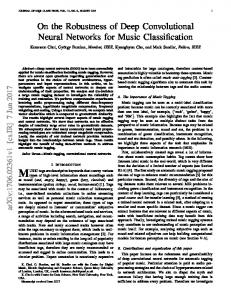
Fig. 1: Comparisons of the speedup of different architectures. This plot shows 2.7× faster training when using 3 × 3 kernels using cuDNN v5.x.

It is very important to avoid rapid downsampling or pooling, especially in early layers. Similar suggestion has also been TABLE I: Improved performance by utilizing cuDNN v7.x. given by [8, 28, 29]. To increase the network’s discriminability k80+cuDNN 6 P100+ cuDNN 6 v100+cuDNN 7 power, more information needs to be made available. This can 2.5x + CNN 100 200 600 be achieved either by a larger dataset (i.e., collecting more 3x + LSTM 1x 2x 6x data, or using augmentation) or utilizing available information more efficiently in the form of larger feature-maps and better information pools. Techniques, such as Inception [3, 7, 8, 16], in the architecture. Since the use of max-pooling will distort inter layer connectivity including residual connections [2], the exact location, excessive appliance of such layer would Dense connections [6], and pooling fusion [56], are examples negatively impact the performance in some applications, such as of more complex ways of providing better information pools. semantic segmentation and object detection. Proper application However, at the very least in its most basic form, an architecture of pooling both results in obtaining translation invariance, can achieve better information pool without such complex and imposes less memory and computation overheads. It also techniques as well. If larger dataset is not available or feasible, needs to be noted that the pooling operation, in its essence the existing training samples must be efficiently utilized. Larger is different than simple downsampling. It is usually theorized feature-maps, especially in the early layers, provide more that a convolutional layer can “learn” the pooling operation valuable information in the network compared to the smaller better. The notion that a pooling operation can be learned ones. With the same depth and number of parameters, a network in a network is correct and have already been tried many that utilizes larger feature-maps achieves a higher accuracy times [15, 56, 59, 60], however, examples such as strided [4, 8, 28]. Therefore, instead of increasing the complexity of a convolutions [42] which are convolutions with bigger strides, network by increasing its depth and its number of parameters, are far from doing that. Techniques such as strided convolution one can leverage better results by simply using larger input thus do not yield the same effect as a pooling operation, since a dimensions or avoiding rapid early downsampling. This is a simple convolution layer with rectified linear activation cannot good technique to keep the complexity of the network in check by itself implement a p-norm computation [42]. Furthermore and to increase the accuracy. Similar observation has been It is argued [42] that the improvement caused by pooling reported by [3, 4, 8] as well. Utilizing larger feature-maps is solely because of the downsampling and thus, one can to create more information pools can result in large memory replace a pooling operation with a strided convolution. However, consumption despite having a small number of parameters. A our empirical results and further intuitions, which result in good example of such practice can be observed in DenseNet improved performance by pooling (explained later), prove [6], from which a model (DenseNet-BC, L = 100, k = 12, otherwise. This is more visible in our tests, where with the with 0.8M parameters) takes more than 8 gigabytes of video same number of parameters, the architecture with simple maxmemory (or VRAM). Although such memory consumption in pooling always outperforms the strided convolution counterpart. part can be attributed to the inefficient implementation, still a This is thoroughly addressed in the experiments section. great deal of that is present even after intensive optimization. Other instances can be seen in [2] and [9] that utilize many layers with large feature-maps. This shows that part of these E. Maximum Performance Utilization architectures success is because of the information pool that Considering implementation details and recent improvements is being provided for each semantic level using an increased in the underlying libraries, one can simply design better number of layers with feature maps of the same size (without performing and more efficient architectures. For instance, being downsampled). Moreover, other than data-augmentation, using 3 × 3 filters, besides its already known benefits [4], which has the most influential role in achieving translation allows to achieve a substantial boost in performance, when invariance [57], (max-)pooling plays an important role in using NVIDIA’s Cudnnv5.x library or higher. This is a speed reducing the sensitivity of the output to shift and distortions up of about 2.7× compared to the former v4 version. The [39]. It also helps achieving translation invariance to some performance boost can be witnessed in newer versions such as extend [28, 58]. Scherner et al. [58] show that max-pooling Cudnnv7.x as well. This is illustrated in Figure 1 and Table I. operation is vastly superior for capturing invariances in image- The ability to harness every amount of performance is crucial, like data, compared to a subsampling operations. Therefore, it is when it comes to production and industry. Whereas, using larger important to have reasonably enough number of pooling layers kernels such as 5 × 5 and 7 × 7 tend to be disproportionally

7

more expensive in terms of computation. For example, a policy leads to inefficient convergence, wasting network re5 × 5 convolution with n filters over a grid with m filters sources. Simple things, such as learning rates and regularization is 25/9 = 2.78 times more computationally expensive than a methods, usually have an adverse effect if not tuned correctly. 3 × 3 convolution with the same number of filters. Of course, a Therefore, it is first suggested to use an automated optimization 5 × 5 filter can capture dependencies between signals activation policy to run quick tests and when the architecture is finalized, of units further away in the earlier layers, so a reduction of the the optimization policy is carefully tuned to maximize network geometric size of the filters comes at a larger cost [8]. Besides performance. It is essential to note that when testing a new the performance point of view, on one hand larger kernels do feature or applying a change, everything else (i.e., all other not provide the same efficiency per parameter as a 3 × 3 kernel settings) remain unchanged throughout the whole experimental does. It may be interpreted that since larger kernels capture round. For example, when testing 5 × 5 vs. 3 × 3, the overall a larger area of neighborhood in the input, they may help network entropy must remain the same. It is usually neglected suppressing noise to some extend and thus capturing better in different experiments and features are not tested in isolation features. However, in practice the overhead they impose in or better said, under a fair and equal condition which ultimately addition to the loss in information they cause makes them not an results in a not-accurate or, worse, a wrong deduction. ideal choice. Furthermore, larger kernels can be factorized into smaller ones [8], and therefore using them makes the efficiency per parameter to decline, causing unnecessary computational H. Dropout Utilization burden. Substituting larger kernels with smaller ones is also Using dropout has been an inseparable part of nearly all previously investigated in [7, 8]. Smaller kernels, on the other recent deep architectures, often considered as an effective hand, do not capture local correlations as well as 3 × 3 kernels. regularizer. Dropout is also interpreted as an ensemble of Detecting boundaries and orientations are better done using a several networks, which are trained on different subsets of 3×3 kernel in earlier layers. A cascade of 3×3 can also replace the training data. It is believed that the regularization effect any larger one and yet achieve similar effective receptive field. of dropout in convolutional layers is mainly influential for In addition, as discussed, they lead to better performance gain. robustness to noisy inputs. To avoid overfitting, as instructed by [40], half of the feature detectors are usually turned off. However, this often causes the network to take a lot more to F. Balanced Distribution Scheme converge or even underfit, and therefore in order to compensate Typically, allocating neurons disproportionally throughout for that, additional parameters are added to the network, the network is not recommended, because the network would resulting in higher overhead in computation and memory face information shortage in some layers and operate inefusage. Towards better utilizing this technique, there have been fectively. For example, if not enough capacity is given to examples such as [42] that have used dropout after nearly all early layers to provide low-level features, or middle layers to convolutional layers rather than only fully connected layers, provide middle-level features, the final layers would not have seemingly to better fight overfitting of their large (at the time) access to sufficient information to build on. This applies to network. Recently [6] also used dropout with all convolutional all semantic levels in a network, i.e., if there is not enough layers with less dropout ratio. Throughout our experiments capacity in the final layers, the network cannot provide higher and also in accordance to the findings of [61], we found level abstractions needed for accurate deduction. Therefore, to that applying dropout to all convolutional layers improves increase the network capacity (i.e., number of neurons) it is the accuracy and generalization power to some extent. This best to distribute the neurons throughout the whole network, can be attributed to the behavior of neurons in different layers. rather than just fattening one or several specific layers [8]. The One being the Dead ReLU issue, where a percentage of the degradation problem that occurs in deep architectures stems whole network never gets activated and thus a substantial from several causes, including the ill-distributed neurons. As network capacity is wasted. The dead ReLU issue can be the network is deepened, properly distributing the processing circumvented by using several methods (e.g., by using other capacity throughout the network becomes harder and this often variants of ReLU nonlinearity family [11, 20]). Another way is the cause for some deeper architectures under-performing to avoid this issue is to impose sparsity by randomly turning against their shallower counterparts. This is actually what arises off some neurons, so that their contribution that may cause to PLD and PLS issues. we address this in the experiments incoming input to the next neurons get negative, cancel out and section in details. Using this scheme, all semantic levels in thus avoid the symptom. The dropout procedure contributes the network will have increased capacity and will contribute to this by randomly turning off some neurons, and thus helps accordingly to the performance, whereas the other way around in avoiding the dead ReLU issue (see Figures 2 and 3). will only increase some specific levels of capacity, which will Additionally, for other types of nonlinearities incorporated most probably be wasted. in deep architectures, dropout causes the network to adapt to new feature combinations and thus improves its robustness G. Rapid Prototyping In Isolation (see Figure 4). It also improves the distributed representation It is very beneficial to test the architecture with different effect [40] by preventing complex co-adaptions. This can be learning policies before altering it. Most of the times, it is observed in early layers, where neurons have similar mean not the architecture that needs to be changed, rather it is the values, which again is a desirable result, since early layers in optimization policy that does. A badly chosen optimization a CNN architecture capture common features. This dropout

8

With dropout Without dropout

100

50

0 1

11

21

31

41

51

61

67

Fig. 2: Layer 1 neuron activations with and without dropout. More neurons are frequently activated when dropout is used, which means more filters are better developed. procedure improves the generalization power by allowing better sparsity. This can be seen by visualizing the neurons activation in higher layers, which shows more neurons are activated around zero [61] (see Figure 5).

(a) With dropout.

(b) Without dropout.

Fig. 3: When dropout is used, all neurons are forced to take part and thus less dead neurons occur. It also results in the development of more robust and diverse filters.

(a) layer 13, using dropout.

(b) layer 13, using no dropout.

Fig. 5: More neurons are activated around 0 when dropout is used which means more sparsity.

propose a variation, denoted as SAF-pooling, which provides the best performance compared to conventional max-, averagepooling operations. SAF-pooling is essentially the max-pooling operation carried out before a dropout operation. If we consider the input as an image, pooling operation provides a form of spatial transformation invariance, as well as reducing the computational complexity for the upper layers. Furthermore, different images of the same class often do not share the same features due to the occlusion, viewpoint changes, illumination variation, and so on. Therefore, a feature which plays an important role in identification of a class in an image may not appear in different images of the same class. When maxpooling is used alongside (before) dropout, it simulates these cases by dropping high activations deterministically(since high activations are already pooled by max-pooling), acting as if these features were not present This procedure of dropping the maximum activations simulates the case where some important features are not present due to occlusion or other types of variations. Therefore, turning off high activations helps other less prominent but as important features to participate better. The network also gets a better chance of adapting to new and more diverse feature compositions. Furthermore in each feature-map, there may be different instances of a feature, and by doing so, those instances can be further investigated, unlike average pooling that averages all the responses feature-mapwise. This way, all those weak responses get the chance to be improved and thus take a more prominent role in shaping the more robust feature detector. This concept is visualized and explained in more details in supplementary material.

(a) Filters learned in the first layer, (b) Filters learned in the first layer, when dropout is used. when dropout is not used.

Fig. 4: When dropout is not used, filters are not as vivid and more dead units are encountered, which is an indication of the presence of more noise.

J. Final Regulation Stage

While we try to formulate the best ways to achieve better accuracy in the form of rules or guidelines, they are not necessarily meant to be aggressively followed in all cases. I. Simple Adaptive Feature Composition Pooling These guidelines are meant to help achieve a good compromise Max- and average-pooling are two methods for pooling op- between performance and the imposed overhead. Therefore, it eration that have been widely in use by nearly all architectures. is better to start by designing the architecture according to the While different architectures achieved different satisfactory above principles, and then altering the architecture gradually to results by using them and also many other variants [56], we find the best compromise between performance and overhead.

9

BN

BN

SC

3

128

3

66

Conv. 2, 3 & 4

Conv. 1

3

192

×3

3

3

SC

BN

SC

2

3

3

192

2

BN

SC

×4

3

Max Pooling

Conv. 6, 7, 8 & 9

Conv. 5

3

BN 3

288 3

SC

2

BN

2

3

288

Max Pooling

SC

BN 355

3

Conv. 10

Conv. 11

BN

SC

SC

3

432

3

3

3 Conv. 13

Conv. 12

Global Max Pooling

Inner Product

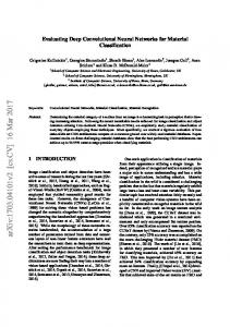
Fig. 6: SimpNet base architecture with no dropout. IV. S IMP N ET

V. E XPERIMENTAL R ESULTS In this section, several experiments are setup to show the significance of the introduced principles. To this end, results are generated without any hyperparameter tuning. These experiments are conducted using variants of our simple architecture. The overall architecture is the same as the one introduced in Section IV with slight changes in the architecture for two reasons, first to make it easier to conduct fair tests between different usecases, and second to provide more diversity in terms of the architecture essence. For example, we tried architectures with different depth and different number of parameters. Therefore, in each experiment, a different version of this network is used with an emphasis on the principle in question. Also, different cases within an experiment use the same architecture and optimization policy so that the test reflects only the changes required by the principle. We report the number of layers and parameters when evaluating each architecture, to see the effect of varying depth with fixed number of parameters for the same network. We present our experimental results in the following subsections, in which two different types of experiments are designed: first to evaluate the principles outlined in Section III, and then to assess the performance of the proposed architecture based on those principles (i.e., SimpNet) compared to several leading architectures.

Based on the principles mentioned above, we build a simple convolutional network with 13 layers. The network employs a homogeneous design utilizing 3 × 3 filters for convolutional layers and 2×2 filters for pooling operations. Figure 6 illustrates the proposed architecture. To design the network based on the above principles, we first specified the maximum depth allowed, to assess the architecture characteristics in comparisons with other deeper and wider counterparts. Following the first rule, we started by creating a thin but deeper architecture with 10 layers, then gradually increased its width to the point where no improvements were witnessed. The depth is then increased, and at the same time the last changes related to the width are reverted back. The experiments are reiterated and the width is increased gradually (related to the first rule and rapid prototyping). During this process, we kept the width of all layers proportional and avoided any excessive allocation or lack thereof (balanced distribution scheme). In order to manage this criteria, we designed layers in groups with similar characteristics, i.e., the same number of featuremaps and feature-map sizes (homogeneous groups). To enable the extraction and preservation of as much information as possible, we used pooling operation sparingly, thus placing a pooling layer after each 5 layers. This lets the network to preserve the essential information with increased nonlinearity A. Implementation Details (maximum information utilization). The exact locations where The experiments concerning the design principles use pooling should be placed can be easily determined through CIFAR10 benchmark dataset, however, the second set of a few tests. Since groups of homogeneous layers are used, experiments are run on 4 major benchmarking datasets namely, placing poolings after each group makes it an easy experiment. CIFAR10, CIFAR100, SVHN and MNIST. CIFAR10/100 We used 3 × 3 filters to preserve local information maximally, datasets [62] include 60,000 color images, of which 50,000 and also to utilize underlying performance optimizations in belong to the training set and the rest are reserved for testing cuDNN library (maximum performance). We then ran several (validation), with 10 and 100 distinct classes, respectively. The experiments in order to assess different network characteristics, classification performance is evaluated using top-1 error. The and in order to avoid sweeping unintentional details affecting SVHN dataset [63] is a real-world image dataset, obtained the final result, we ran experiments in isolation, i.e., when an from house numbers in Google Street View images. It consists experiment is being run, all criteria are locked. Finally the of 630,420 32 × 32 color images, 73,257 of which are used network is revised in order to resolve specific internal limits, for training, 26,032 images are used for testing and the other i.e., memory consumption and number of parameters (final 531,131 images are used for extra training. The MNIST dataset regulation stage). [39] also consists of 70,000 28 × 28 grayscale images of

10

TABLE II: Gradual expansion of the number of layers. Network Properties Arch1, 8 Layers Arch1, 9 Layers Arch1, 10 Layers Arch1, 13 Layers

Parameters 300K 300K 300K 300K

Accuracy (%) 90.21 90.55 90.61 89.78

handwritten digits, 0 to 9, with 60,000 images used for training and 10,000 for testing. We used Caffe framework [64] for training our architecture and ran our experiments on a system with Intel Corei7 4790K CPU, 20 Gigabytes of RAM and NVIDIA GTX1080 GPU. B. Examining the Design Intuitions The first set of experiments involve examining the design principles, ran on CIFAR10 [62] dataset. Gradual Expansion and Minimum Allocation: Table II shows how gradually expanding the network helps obtaining better performance. Increasing the depth up to a certain point improves accuracy (up to 10 layers) and then after that it starts to degrade the performance. It is interesting to note that a 10-layer network is outperforming the same network with 13 layers. While in the next experiment(s), a deeper network is outperforming a shallower one with much fewer parameters. As already explained in the principles, namely in Subsections III-A and III-F, one of the root causes that affects deeper architectures is an ill-distribution of processing capacity and more specifically the PLD/PLS issues, which can be seen in Table II and III respectively. These issues are indications of how a specific architecture manifests its needs, including more processing or representational capacity. It may be argued that the shallower architectures can still accommodate more capacity until they meet their true saturation point and, therefore, the difference in accuracy may be attributed to illdistribution, rather than saturation (i.e., PLD/PLS). PLD/PLS are themselves manifestation of issues in proper distribution of processing units. Moreover, saturation is a process, which starts at some point and, as continues, it becomes more prominent. Our point is to give such impression and thus do not get into the specifics of finding the upper limit of an architecture saturation point. The networks used for II experiments are variants of SimpNet with different depths, denoted by Arch1 in the table. More information concerning architectures and their overall topology is given in the supplementary material. In addition to the first test, Table III shows how a deeper network with fewer number of parameters works better than its shallower but wider counterparts. A deeper architecture can develop more interesting functions and thus the composition of many simpler functions can yield better inference, when properly capaciated. This is why despite the difference in the number of parameters, the deeper one is performing better. This experiment shows the importance of minimum allocation in the gradual expansion scheme. The networks used in III are variants of Arch1. Table IV demonstrates the results concerning balanced distribution of processing units throughout the architecture and how it excels against the ill-distributed counterpart. Networks used for IV use variants of [43], which

TABLE III: Shallow vs. Deep (related to Minimum Allocations), showing how a gradual increase can yield better performance with fewer number of parameters. Network Properties Arch1, 6 Layers Arch1, 10 Layers

Parameters 1.1M 570K

Accuracy (%) 92.18 92.23

TABLE IV: Balanced distribution scheme is demonstrated by using two variants of SimpNet architecture with 10 and 13 layers, each showing how the difference in allocation results in varying performance and ultimately improvements for the one with balanced distribution of units. Network Properties Arch2, 10 Layers (wide end) Arch2, 10 Layers (balanced width) Arch2, 13 Layers (wide end) Arch2, 13 Layers (balanced width)

Parameters 8M 8M 128K 128K

Accuracy (%) 95.19 95.51 87.20 89.70

we call Arch2 from which The first 10 layers are used for the 10-layer architecture and the 13-layer architecture is slimmed to have 128K parameters for the second test. Maximum Information Utilization: The Results summarized in the Table V show the effect of delayed pooling in an architecture, and demonstrate how utilizing more information in the form of bigger feature-maps can help the network to achieve higher accuracy. This table shows a variant of SimpNet with 13 layers and only 53K parameters, along with its performance with and without delayed pooling. We call this architecture Arch3. To assess the effect in question, one pooling operation is applied each time at different layers and everything else is kept fixed. L5, L3 and L7 refer to layer 5, 3 and 7, respectively. The results indicate an improvement compared to the initial design. Strided convolution vs. Maxpooling: Table VI demonstrates how a pooling operation regardless of architecture, dataset and number of parameters, outperforms the strided convolution. This proves our initial claim and thus nullifies the theory which implies 1. downsampling is what that matters, 2. strided convolution performs better than pooling. Apart from these, form the design point of view, strided convolution imposes more unwanted and unplanned overhead to the architecture and thus contradicts the principled design and notably gradual expansion and minimum allocation. To be more precise, it introduces adhoc allocation strategy, which in-turn introduces PLD issues into the architecture. This is further explained in supplementary material. Correlation Preservation: Table VII shows the effect of correlation preservation, and how a 3 × 3 architecture is better than its counterpart utilizing a bigger kernel size but with the same number of parameters. Table VIII illustrates the same concept on different architectures and demonstrates how 1 × 1, 2 × 2 and 3 × 3 compare with each other at different layers. As it can be seen, applying 1 × 1 on earlier layers has a bad effect on the performance, while in the middle layers it is not as bad. It is also clear that 2 × 2 performs better than 1 × 1 in all cases, while 3 × 3 filters outperform both of them. Here we ran several tests using different kernel sizes, with two different variants, one having 300K and the other

11

TABLE V: The effect of using pooling at different layers. TABLE VII: Accuracy for different combinations of kernel Applying pooling early in the network adversely affects the sizes and number of network parameters, which demonstrates performance. how correlation preservation can directly effect the overall accuracy. Network Properties Parameters Accuracy (%) Arch3, L5 default Arch3, L3 early pooling Arch3, L7 delayed pooling

53K 53K 53K

79.09 77.34 79.44

TABLE VI: Effect of using strided convolution (†) vs. Maxpooling (∗). Max-pooling outperforms the strided convolution regardless of specific architecture. First three rows are tested on CIFAR100 and two last on CIFAR10. Network Properties SimpNet∗ SimpNet∗ SimpNet† ResNet∗ ResNet†

Depth 13 15 15 32 32

Parameters 360K 360K 360K 460K 460K

Accuracy (%) 69.28 68.89 68.10 93.75 93.46

Network Properties Arch4, 3 × 3 Arch4, 3 × 3 Arch4, 5 × 5 Arch4, 7 × 7 Arch4, 7 × 7 Arch4, 7 × 7

Parameters 300K 1.6M 1.6M 300K.v1 300K.v2 1.6M

Accuracy (%) 90.21 92.14 90.99 86.09 88.57 89.22

TABLE VIII: Different kernel sizes applied on different parts of a network affect the overall performance, i.e., the kernel sizes that preserve the correlation the most yield the best accuracy. Also, the correlation is more important in early layers than it is for the later ones. Network Properties Arch5, Arch5, Arch5, Arch5,

13 Layers, 1 × 1 vs. 2 × 2 (early layers) 13 Layers, 1 × 1 vs. 2 × 2 (middle layers)

Params 128K 128K 128K 128K

Accuracy (%) 87.71 vs. 88.50 88.16 vs. 88.51 89.45 vs. 89.60 89.30 vs. 89.44

13 Layers, 1 × 1 vs. 3 × 3 (smaller vs. bigger end-avg) 1.6M parameters. Using 7 × 7 in an architecture results in 11 Layers, 2 × 2 vs. 3 × 3 (bigger learned feature-maps) more parameters, therefore in the very same architecture with 3 × 3 kernels, 7 × 7 results in 1.6M parameters. Also, to TABLE IX: The importance of experiment isolation using the decrease the number of parameters, layers should contain fewer same architecture once using 3×3 and then using 5×5 kernels. neurons. Therefore, we created two variants of 300K parameter Network Properties Accuracy (%) architecture for the 7 × 7 based models to both demonstrate the Use of 3 × 3 filters 90.21 effect of 7 × 7 kernel and to retain the computation capacity Use of 5 × 5 instead of 3 × 3 90.99 throughout the network as close as possible between the two counter parts (i.e., 3 × 3 vs. 7 × 7). On the other hand, we TABLE X: Wrong interpretation of results when experiments increased the base architecture from 300K to 1.6M for testing are not compared in equal conditions (Experimental isolation). 3 × 3 kernels as well. Table VII shows the results for these Network Properties Accuracy (%) architectures, in which the 300K.v1 architecture is an all 7 × 7 Use of 5 × 5 filters at the beginning 89.53 Use of 5 × 5 filters at the end 90.15 kernel network with 300K parameters (i.e., the neurons per layer are decreased to match the 300K limit). The 300K.v2 is the same architecture with 7 × 7 kernels only in the first TABLE XI: Using SAF-pooling operation improves architecture two layers, while the rest use 3 × 3 kernels. This is done, so performance. Tests are run on CIFAR10. that the effect of using 7 × 7 filters are demonstrated, while Network Properties Accuracy (%) With–without SAF Pooling SqueezeNetv1.1 88.05(avg)–87.74(avg) most layers in the network almost has the same capacity as SimpNet 94.76–94.68 their counterparts in the corresponding 3 × 3-based architecture. Finally, the 7×7 1.6M architecture is the same as the 3×3 300K architecture, in which the kernels are replaced by 7 × 7 ones again the number of parameters and thus network capacity is and thus resulted in increased number of parameters (i.e., 300K neglected. The example test was to determine whether placing became 1.6M). Therefore, we also increased the 3 × 3-based 5 × 5 filters at the beginning of the network is better than architecture to 1.6, and ran a test for an estimate on how each placing it at the end. Again here the results suggest that of these work in different scenarios. We also used a 5 × 5 1.6M the second architecture should be preferred, but at a closer parameter network with the same idea and reported the results. inspection, it is cleared that the first architecture has only 412K The network used for this test is the SimpNet architecture, parameters, while the second one uses 640K parameters. Thus, with only 8 layers, denoted by Arch4. The networks used in the assumption is not valid because of the difference between Table VIII are also variants of SimpNet with slight changes to the two networks capacities. the depth or number of parameters, denoted by Arch5. SAF-pooling: In order to assess the effectiveness of our Experiment Isolation: Table IX shows an example of intuition concerning Section III-I, we further ran a few tests invalid assumption, when trying different hyperparameters. In using different architectures with and without SAF-pooling the following, we test to see whether 5 × 5 filters achieve better operation on CIFAR10 dataset. We used SqueezeNetv1.1 and accuracy against 3 × 3 filters. Results show a higher accuracy our slimmed version of the proposed architecture to showcase for the network that uses 5 × 5 filters. However, looking at the improvement. Results can be found in Table XI. the number of parameters in each architecture, it is clear that the higher accuracy is due to more parameters in the second C. SimpNet Results on Different Datasets architecture. The first architecture, while cosmetically the same SimpNet performance is reported on CIFAR-10/100 [62], as the second one, has 300K parameters, whereas the second SVHN [63], and MNIST [39] datasets to evaluate and compare one has 1.6M. A second example can be seen in Table X, where our architecture against the top ranked methods and deeper

12

TABLE XII: Top CIFAR10-100 results. Method VGGNet(16L) [65]/Enhanced ResNet-110L / 1202L [2] * SD-110L / 1202L [66] WRN-(16/8)/(28/10) [9] DenseNet [6] Highway Network [37] FitNet [52] FMP* (1 tests) [14] Max-out(k=2) [15] Network in Network [41] DSN [67] Max-out NIN [68] LSUV [69] SimpNet SimpNet

#Params 138m 1.7/10.2m 1.7/10.2m 11/36m 27.2m N/A 1M 12M 6M 1M 1M N/A 5.48M 8.9M

CIFAR10 91.4 / 92.45 93.57 / 92.07 94.77 / 95.09 95.19 / 95.83 96.26 92.40 91.61 95.50 90.62 91.19 92.03 93.25 94.16 95.49/95.56 95.89

CIFAR100 74.84/72.18 75.42 / 77.11/79.5 80.75 67.76 64.96 73.61 65.46 64.32 65.43 71.14 N/A 78.08 79.17

TABLE XIII: MNIST results without data-augmentation. Method Batch-normalized Max-out NIN [68] Max-out network (k=2) [15] Network In Network [41] Deeply Supervised Network [67] RCNN-96 [70] SimpNet

Error rate 0.24% 0.45% 0.45% 0.39% 0.31% 0.25%

slimmed version with only 300K parameters could achieve an error rate of 1.95%. TABLE XIV: Comparisons of performance on SVHN dataset. Method Network in Network[41] Deeply Supervised Net[67] ResNet[2] (reported by [66] (2016)) ResNet with Stochastic Depth[66] DenseNet[6] Wide ResNet[9] SimpNet

Error rate 2.35 1.92 2.01 1.75 1.79-1.59 2.08-1.64 1.648

4) Architectures with fewer number of parameters: Some architectures cannot scale well, when their processing capacity is decreased. This shows the design is not robust enough to efficiently use its processing capacity. We tried a slimmed version of our architecture, which has only 300K parameters to see how it performs and whether it is still efficient. Table XV shows the results for our architecture with only 300K and 600K parameters, in comparison to other deeper and heavier architectures with 2 to 20 times more parameters. As it can be seen, our slimmed architecture outperforms ResNet and WRN with fewer and also the same number of parameters on CIFAR10/100.

models that also experimented on these datasets. We only used simple data augmentation of zero padding, and mirroring on CIFAR10/100. Other experiments on MNIST [39], SVHN TABLE XV: Slimmed version results on CIFAR10/100 datasets. [63] and ImageNet [5] datasets are conducted without dataModel Param CIFAR10 CIFAR100 Ours 300K - 600K 93.25 - 94.03 68.47 - 71.74 augmentation. In our experiments we used one configuration for Maxout [15] 6M 90.62 65.46 all datasets and did not fine-tune anything except for CIFAR10. DSN [67] 1M 92.03 65.43 We did this to see how this configuration can perform with no ALLCNN [42] 1.3M 92.75 66.29 dasNet [71] 6M 90.78 66.22 or slightest changes in different scenarios. ResNet [2] (Depth32, tested by us) 475K 93.22 67.37-68.95 1) CIFAR10/100: Table XII shows the results achieved by WRN [9] 600K 93.15 69.11 different architectures. We tried two different configurations NIN [41] 1M 91.19 — for CIFAR10 experiment, one with no data-augmentation, i.e., no zero-padding and normalization and another one using data-augmentation, we achieved 95.26% accuracy with no VI. C ONCLUSION zeropadding and normalization and achieved 95.56% with zero-padding. By just naively adding more parameters to our In this paper, we proposed a set of architectural design princiarchitecture without further fine-tuning or extensive changes ples, a new pooling layer, detailed insight about different parts to the architecture, we could easily surpass all WRN results in design, and finally introduced a new lightweight architecture, ranging from 8.9M (with the same model complexity) to 11M, SimpNet. SimpNet outperforms deeper and more complex to 17M and also 36M parameters on CIFAR10/100 and get very architectures in spite of having considerably fewer number of close to its state-of-the-art architecture with 36M parameters parameters and operations, although the intention was not to set on CIFAR100. This shows that the architecture, although with a new state-of-the-art, rather, showcasing the effectiveness of fewer number of parameters and layers, is still capable beyond the introduced principles. We showed that a good design should what we tested with a limited budget of 5M parameters and, be able to efficiently use its processing capacity and that our thus, by just increasing the number of parameters, it can slimmed version of the architecture with much fewer number match or even exceed the performance of much more complex of parameters outperforms deeper and heavier architectures as architectures. well. Intentionally, limiting ourselves to a few layers and basic 2) MNIST: On this dataset, no data-augmentation is used, elements for designing an architecture allowed us to overlook and yet we achieved the second highest score even without the unnecessary details and concentrate on the critical aspects fine-tuning. [18] achieved state-of-the-art with extreme data- of the architecture, keeping the computation in check and augmentation and an ensemble of models. We also slimmed achieving high efficiency, along with better insights about the our architecture to have only 300K parameters and achieved design process and submodules that affect the performance the 99.73%. Table XIII shows the result. most. As an important direction for the future works, there is a 3) SVHN: Like [15, 41, 66], we only used the training and calling need to study the vast design space of deep architectures testing sets for our experiments and did not use any data- in an effort to find better guidelines for designing more efficient augmentation. Best results are presented in Table XIV. Our networks.

13

ACKNOWLEDGMENT The authors would like to thank Dr. Ali Diba, CTO of Sensifai, for his invaluable help and cooperation, and Dr. Hamed Pirsiavash, Assistant Professor at University of Maryland-Baltimore County (UMBC), for his insightful comments on strengthening this work.

R EFERENCES [1] Y. Guo, Y. Liu, A. Oerlemans, S. Lao, S. Wu, and M. S. Lew, “Deep learning for visual understanding: A review,” Neurocomputing, 2015. [2] K. He, X. Zhang, S. Ren, and J. Sun, “Deep residual learning for image recognition,” CoRR, vol. abs/1512.03385, 2015. [3] C. Szegedy, W. Liu, Y. Jia, P. Sermanet, S. Reed, D. Anguelov, D. Erhan, V. Vanhoucke, and A. Rabinovich, “Going deeper with convolutions,” in CVPR, pp. 1–9. [4] K. Simonyan and A. Zisserman, “Very deep convolutional networks for large-scale image recognition,” CoRR, vol. abs/1409.1556, 2014. [5] O. Russakovsky, J. Deng, H. Su, J. Krause, S. Satheesh, S. Ma, Z. Huang, A. Karpathy, A. Khosla, M. Bernstein, A. C. Berg, and L. Fei-Fei, “Imagenet large scale visual recognition challenge,” in ICCV, vol. 115, pp. 211–252, 2015. [6] G. Huang, Z. Liu, K. Q. Weinberger, and L. van der Maaten, “Densely connected convolutional networks,” arXiv preprint arXiv:1608.06993, 2016. [7] C. Szegedy, S. Ioffe, V. Vanhoucke, and A. Alemi, “Inception-v4, inceptionresnet and the impact of residual connections on learning,” arXiv preprint arXiv:1602.07261, 2016. [8] C. Szegedy, V. Vanhoucke, S. Ioffe, J. Shlens, and Z. Wojna, “Rethinking the inception architecture for computer vision,” in CVPR, pp. 2818–2826. [9] S. Zagoruyko and N. Komodakis, “Wide residual networks,” arXiv preprint arXiv:1605.07146, 2016. [10] X. Glorot and Y. Bengio, “Understanding the difficulty of training deep feedforward neural networks,” in AISTATS, vol. 9, pp. 249–256. [11] K. He, X. Zhang, S. Ren, and J. Sun, “Delving deep into rectifiers: Surpassing human-level performance on imagenet classification,” in CVPR, pp. 1026–1034. [12] D. Mishkin and J. Matas, “All you need is a good init,” arXiv preprint arXiv:1511.06422, 2015. [13] A. M. Saxe, J. L. McClelland, and S. Ganguli, “Exact solutions to the nonlinear dynamics of learning in deep linear neural networks,” arXiv:1312.6120, 2013. [14] B. Graham, “Fractional max-pooling,” vol. ArXiv e-prints, December 2014a, 2014. [15] I. J. Goodfellow, D. Warde-Farley, M. Mirza, A. Courville, and Y. Bengio, “Maxout networks,” in ICML, vol. 28, pp. 1319–1327, 2013. [16] S. Ioffe and C. Szegedy, “Batch normalization: Accelerating deep network training by reducing internal covariate shift,” CoRR, vol. abs/1502.03167, 2015. [17] S. Wager, S. Wang, and P. S. Liang, “Dropout training as adaptive regularization,” in NIPS, pp. 351–359. [18] L. Wan, M. Zeiler, S. Zhang, Y. L. Cun, and R. Fergus, “Regularization of neural networks using dropconnect,” in ICML, pp. 1058–1066. [19] D.-A. Clevert, T. Unterthiner, and S. Hochreiter, “Fast and accurate deep network learning by exponential linear units (elus),” arXiv preprint arXiv:1511.07289, 2015. [20] A. L. Maas, A. Y. Hannun, and A. Y. Ng, “Rectifier nonlinearities improve neural network acoustic models,” in ICML, vol. 30. [21] V. Nair and G. E. Hinton, “Rectified linear units improve restricted boltzmann machines,” in ICML, pp. 807–814. [22] K. Alex, I. Sutskever, and E. H. Geoffrey, “Imagenet classification with deep convolutional neural networks,” in NIPS, pp. 1097–1105, 2012. [23] R. Wu, S. Yan, Y. Shan, Q. Dang, and G. Sun, “Deep image: Scaling up image recognition,” CoRR, vol. abs/1501.02876, 2015. [24] B. Xu, N. Wang, T. Chen, and M. Li, “Empirical evaluation of rectified activations in convolutional network,” arXiv preprint arXiv:1505.00853, 2015. [25] B. Zoph, V. Vasudevan, J. Shlens, and Q. V. Le, “Learning transferable architectures for scalable image recognition,” arXiv preprint arXiv:1707.07012, 2017. [26] S. Han, H. Mao, and W. J. Dally, “Deep compression: Compressing deep neural network with pruning, trained quantization and huffman coding,” CoRR, abs/1510.00149, vol. 2, 2015. [27] M. Rastegari, V. Ordonez, J. Redmon, and A. Farhadi, “Xnor-net: Imagenet classification using binary convolutional neural networks,” in ECCV, pp. 525–542, Springer. [28] K. He and J. Sun, “Convolutional neural networks at constrained time cost,” in CVPR, pp. 5353–5360. [29] F. N. Iandola, S. Han, M. W. Moskewicz, K. Ashraf, W. J. Dally, and K. Keutzer, “Squeezenet: Alexnet-level accuracy with 50x fewer parameters and< 0.5 mb model size,” arXiv preprint arXiv:1602.07360, 2016. [30] L. N. Smith and N. Topin, “Deep convolutional neural network design patterns,” arXiv preprint arXiv:1611.00847, 2016. [31] K. Fukushima, “Neural network model for a mechanism of pattern recognition unaffected by shift in position- neocognitron,” ELECTRON. & COMMUN. JAPAN, vol. 62, no. 10, pp. 11–18, 1979. [32] K. Fukushima, “Neocognitron: A self-organizing neural network model for a mechanism of pattern recognition unaffected by shift in position,” Biological cybernetics, vol. 36, no. 4, pp. 193–202, 1980. [33] A. G. Ivakhnenko, “Polynomial theory of complex systems,” IEEE Transactions on Systems, Man, and Cybernetics, no. 4, pp. 364–378, 1971. [34] D. C. Ciresan, U. Meier, L. M. Gambardella, and J. Schmidhuber, “Deep, big, simple neural nets for handwritten digit recognition,” Neural computation, vol. 22, no. 12, pp. 3207–3220, 2010.

[35] D. Cirecsan, U. Meier, J. Masci, and J. Schmidhuber, “A committee of neural networks for traffic sign classification,” in IJCNN, pp. 1918–1921, IEEE. [36] D. CirecsAn, U. Meier, J. Masci, and J. Schmidhuber, “Multi-column deep neural network for traffic sign classification,” Neural Networks, vol. 32, pp. 333–338, 2012. [37] R. K. Srivastava, K. Greff, and J. Schmidhuber, “Highway networks,” arXiv preprint arXiv:1505.00387, 2015. [38] D. Ciregan, U. Meier, and J. Schmidhuber, “Multi-column deep neural networks for image classification,” in CVPR, pp. 3642–3649, IEEE. [39] Y. Lecun, L. Bottou, Y. Bengio, and P. Haffner, “Gradient-based learning applied to document recognition,” Proceedings of the IEEE, vol. 86, pp. 2278–2324, 1998. [40] G. E. Hinton, N. Srivastava, A. Krizhevsky, I. Sutskever, and R. R. Salakhutdinov, “Improving neural networks by preventing co-adaptation of feature detectors,” arXiv preprint arXiv:1207.0580, 2012. [41] M. Lin, Q. Chen, and S. Yan, “Network in network,” CoRR, vol. abs/1312.4400, 2013. [42] J. T. Springenberg, A. Dosovitskiy, T. Brox, and M. A. Riedmiller, “Striving for simplicity: The all convolutional net,” CoRR, vol. abs/1412.6806, 2014. [43] S. H. Hasanpour, M. Rouhani, M. Fayyaz, and M. Sabokrou, “Lets keep it simple: using simple architectures to outperform deeper architectures,” arXiv preprint arXiv:1608.06037, 2016. [44] A. G. Howard, M. Zhu, B. Chen, D. Kalenichenko, W. Wang, T. Weyand, M. Andreetto, and H. Adam, “Mobilenets: Efficient convolutional neural networks for mobile vision applications,” arXiv preprint arXiv:1704.04861, 2017. [45] X. Zhang, X. Zhou, M. Lin, and J. Sun, “Shufflenet: An extremely efficient convolutional neural network for mobile devices,” arXiv preprint arXiv:1707.01083, 2017. [46] D. Eigen, J. Rolfe, R. Fergus, and Y. LeCun, “Understanding deep architectures using a recursive convolutional network,” arXiv preprint arXiv:1312.1847, 2013. [47] K. J. Geras, A.-r. Mohamed, R. Caruana, G. Urban, S. Wang, O. Aslan, M. Philipose, M. Richardson, and C. Sutton, “Blending lstms into cnns,” arXiv preprint arXiv:1511.06433, 2015. [48] H. Larochelle, D. Erhan, A. Courville, J. Bergstra, and Y. Bengio, “An empirical evaluation of deep architectures on problems with many factors of variation,” in ICML, pp. 473–480, ACM. [49] F. Seide, G. Li, and D. Yu, “Conversational speech transcription using contextdependent deep neural networks,” in ISCA. [50] R. K. Srivastava, K. Greff, and J. Schmidhuber, “Training very deep networks,” in NIPS, pp. 2377–2385. [51] G. Urban, K. J. Geras, S. E. Kahou, O. A. S. Wang, R. Caruana, A. Mohamed, M. Philipose, and M. Richardson, “Do deep convolutional nets really need to be deep (or even convolutional)?,” in ICLR, 2017. [52] A. Romero, N. Ballas, S. E. Kahou, A. Chassang, C. Gatta, and Y. Bengio, “Fitnets: Hints for thin deep nets,” arXiv preprint arXiv:1412.6550, 2014. [53] M. D. Zeiler and R. Fergus, Visualizing and Understanding Convolutional Networks, pp. 818–833. Cham: Springer International Publishing, 2014. [54] F. Iandola, M. Moskewicz, S. Karayev, R. Girshick, T. Darrell, and K. Keutzer, “Densenet: Implementing efficient convnet descriptor pyramids,” arXiv preprint arXiv:1404.1869, 2014. [55] Y. LeCun, Y. Bengio, and G. Hinton, “Deep learning,” Nature, vol. 521, no. 7553, pp. 436–444, 2015. [56] C.-Y. Lee, P. W. Gallagher, and Z. Tu, “Generalizing pooling functions in convolutional neural networks: Mixed, gated, and tree,” in AISTATS. [57] E. Kauderer-Abrams, “Quantifying translation-invariance in convolutional neural networks,” 2016. [58] D. Scherer, A. Muller, and S. Behnke, “Evaluation of pooling operations in convolutional architectures for object recognition,” Artificial Neural Networks, pp. 92–101, 2010. [59] C. Gulcehre, K. Cho, R. Pascanu, and Y. Bengio, “Learned-norm pooling for deep feedforward and recurrent neural networks,” in Joint European Conference on Machine Learning and Knowledge Discovery in Databases, pp. 530–546, Springer, 2014. [60] Y. Jia, C. Huang, and T. Darrell, “Beyond spatial pyramids: Receptive field learning for pooled image features,” in Computer Vision and Pattern Recognition (CVPR), 2012 IEEE Conference on, pp. 3370–3377, IEEE, 2012. [61] S. Park and N. Kwak, “Analysis on the dropout effect in convolutional neural networks,” in ACCV, pp. 189–204, Springer. [62] A. Krizhevsky and G. Hinton, “Learning multiple layers of features from tiny images,” 2009. [63] Y. Netzer, T. Wang, A. Coates, A. Bissacco, B. Wu, and A. Y. Ng, “Reading digits in natural images with unsupervised feature learning,” in NIPS workshop, 2011. [64] Y. Jia, E. Shelhamer, J. Donahue, S. Karayev, J. Long, R. Girshick, S. Guadarrama, and T. Darrell, “Caffe: Convolutional architecture for fast feature embedding,” vol. arXiv preprint arXiv:1408.5093, 2014. [65] S. Zagoruyko, “92.45% on cifar-10 in torch,” 2015. [66] G. Huang, Y. Sun, Z. Liu, D. Sedra, and K. Weinberger, “Deep networks with stochastic depth,” arXiv preprint arXiv:1603.09382, 2016. [67] C.-Y. Lee, S. Xie, P. Gallagher, Z. Zhang, and Z. Tu, “Deeply supervised nets,” AISTATS, 2015. [68] Y.-S. C. Jia-Ren Chang, “Batch-normalized maxout network in network,” vol. arXiv:1511.02583v1, 2015. [69] J. M. Dmytro Mishkin, “All you need is a good init,” in ICLR, 2016. [70] M. Liang and X. Hu, “Recurrent convolutional neural network for object recognition,” in CVPR, pp. 3367–3375. [71] M. F. Stollenga, J. Masci, F. Gomez, and J. Schmidhuber, “Deep networks with internal selective attention through feedback connections,” in NIPS, pp. 3545–3553,

S1

Towards Principled Design of Deep Convolutional Networks: Introducing SimpNet (Supplementary Material) Seyyed Hossein Hasanpour, Mohammad Rouhani, Mohsen Fayyaz, Mohammad Sabokrou and Ehsan Adeli

S1. E XTENDED D ISCUSSIONS A. Strided convolution vs. Max-pooling

[1], we propose a variation, denoted as SAF-Pooling, which provides the best performance compared to conventional max, average-pooling operations. SAF-Pooling is essentially the max-pooling operation carried out before a dropout operation.

Table VI (in the main paper) demonstrates how a pooling operation, regardless of architecture, dataset, and number of parameters, outperforms the strided convolution. This goes along our initial claim and also contradicts with the assumption C. SAF-Pooling Intuition which implies (1) Downsampling is what that matters; (2) If the input is considered as an image, pooling operation Strided convolution performs better than pooling. Furthermore, provides a form of spatial transformation invariance as well from the design point of view, strided convolution imposes as reducing the computational complexity for the upper layers. unwanted and unplanned overhead to the architecture and However, by considering the input to the pooling layer as therefore contradicts the principled design and notably gradual a series of different features, which is actually the case expansion and minimum allocation. It introduces ad hoc after appliance of several layers and feature representation allocation which in-turn causes PLD issues in the architecture. possibly getting shrunk, it would be a mechanism which selects Suppose an optimal depth is X with a given budget Y , using prominent features that describe an input identity. In this sense, gradual expansion, one reaches to the depth X using pooling an ideal pooling method is expected to preserve task-related operation, now replacing pooling with strided convolution, information, while discarding irrelevant details. It is noteworthy introduces K layers to the architecture depth, (K is the number that for the first intuition which considers input as an image, an of pooling layers). In the limited budget, the network will overlapping pooling would be desired since the nonoverlapping face PLD, since the balanced distribution is not optimal for pooling would lose considerably more spatial information in the new depth. Furthermore, in order to cope with the PLD the input than its counterpart. However, when this assumption issue, the capacity needs to be increased by a large margin to doesn’t hold, nonoverlapped pooling would be a better choice. accommodate K new layers. The resulting architecture, then, In our experiments, we noted that the nonoverlapping version ultimately under-performs against its counterpart using pooling outperforms the overlapped version by a relatively high margin, operations, since strided convolution does not approximate a two intuitions may explain this improvement: (1) Due to the pooling layer and can only simulate the downsampling part of distributed representation and hierarchical nature of the network, a pooling layer. This can be clearly seen from the obtained and the fact that the neurons at higher level capture high-level results. For the first part of the argument, it can be seen that and abstract features unlike the ones at earlier layers which are the 13-layer architecture, which uses pooling with the same concerned with more low-level features and also (2) Deeper in number of parameters , outperforms the strided version with 15 the architecture, the essence of the input image changes and it layers by a relatively large margin. The 15-layer version also is no more the same input image/representation rather, it is a outperforms the strided counterpart, although both show signs feature-map, each pixel of which denotes a feature being present of PLD, the pooling based architecture performs much better. or not. Aafter some stages, the notion of image would not make For the second part of the argument, a ResNet architecture with sense at all, since the spatial dimension of the input may have 32 layers is tested. ResNet uses strided convolutions and when shrunk so much that the identity inside image can no more be it is altered to use pooling instead it performs much better. recognized (consider a 8×8 grid from a 32×32 pixel image of With the same depth, number of parameters and distribution CIFAR10 dataset). Taking these two points into consideration, scheme, the pooling-based architecture outperforms the strided we are truly dealing with feature-maps in a network especially convolution version. Therefore it is recommended not to use in mid to high layers. Thus, the second intuition seems more strided convolution instead of pooling. plausible, at least when pooling is carried out in the later layers as opposed to earlier ones, where the nonoverlapping B. Simple Adaptive Feature Composition Pooling may matter more because of more image like properties being Max- and average-pooling are the two methods for pool- still available. Furthermore, the first intuition may only apply ing operation that have been widely in use by nearly all to images in applications such as semantic segmentation and architectures. While different architectures achieved different object detection based on current practices, and for other satisfactory results by using them and also many other variants applications such as classification or other strategies in semantic

S2

Stage 1 : Building initial features

Stage 2: Capturing highest activated neurons

1

2

4

8

0

5

1

3

5

8

2

7

1 2

7

9

0

5

6 9

3 0 0 1

6 6 5

3

3

6

2 4 5 1

8

2

5

9

2 9

Stage 3 : Turn off stage High level feature detectors Whisker

Ear

New Feature compositions are developed

Ear

Paw

0.8

.01

.22

.45

.02

.01

.01

.02

.01

.0

.47

.37

Paw

Whisker

Final stage: Adapting to new feature combinations

Cat √

Fig. S1: SAF-Pooling: In this scheme, the network is forced to adapt itself to several different feature combinations through deterministically deactivating some feature responses, so that in cases some features are absent, due to occlusion, viewpoint changes, noise, etc., the network can still carry out its task using other available features. The process happens in several stages. After some mid/high level features are available (Stage 1), most prominent features (responses) are pooled (Stage 2). Then, some of them are deterministically turned off. The network now has to adapt to the absence of some prominent features and therefore develop new feature compositions (Stage 3). After several iterations, less relevant (or irrelevant) features will be gradually replaced by more informative ones as weaker features are more frequently given the chance to be further developed. As the cycle continues, more feature compositions are developed which ultimately results in the network maximizing the capacity utilization, by creating more diverse feature detectors, as more neurons will be sparsely activated and independently learn patterns. segmentation- or detection-based applications, it may not well. Therefore, we followed the second intuition. Another form hold. Moreover, drastic loss of information that is claimed of pooling is average-pooling, but how does it fare with maxto be attributed to nonoverlapped pooling is usually caused pooling in general? Average-pooling takes all activations in a by either drastic usage of pooling operations or frequent uses pooling region into consideration with “equal contributions”. of them in the architecture, such as the cases that can be This may downplay high activations as many low activations encountered in very deep architectures with several pooling are averagely included. Max-pooling, however, only captures layers, to take the computational burden as low as possible. the strongest activations, and disregards all other units in the Therefore, in the absence of such preconceptions/preconditions, pooling region [2]. We noted that the usage of average-pooling the nonoverlapping pooling would not only pose an issue but specifically in early layers adversely affects the accuracy. would also be beneficial, as we experienced in our results as However, in upper layers, it seems the difference between

S3

the two methods (max and average) is much less severe. E. Visualizing SAF-Pooling Furthermore, different images of the same class often do not In order to better demonstrate the underlying idea, and share the same features due to the occlusion, viewpoint changes, how it affects the performance of the network, we have run illumination variation, and so on. Therefore, a feature which some experiments. In the following set of figures we show plays an important role in identification of a class in an image how the the notion of image is drastically changed through a may not appear in different images of the same class. When network especially in higher layers and how this seemingly max-pooling is used alongside (before) dropout, it simulates minor observation plays an important role in developing these cases by dropping high activations deterministically (since better intuitions about the network and how to improve high activations are already pooled by max-pooling), acting as its performance. This observation, in addition to the fact if these features were not present. Placing pooling after dropout, that poolings should not be applied early in the network, simulates the stochastic pooling operation, which turns off any signifies that using overlapped pooling to keep image’s spatial neurons randomly and does not yield the same improvement information does not make much sense, and if they are treated as often. In our experiments, we found that it performs simply as feature-maps, it can lead to simple yet surprising inferior to its counterpart. This procedure of dropping the ways of improvements (i.e., SAF). In Figure S2, a head/neck maximum activations simulates the case where some important detector is being demonstrated. Followed by a max-pooling features are not present due to occlusion or other types of variations. Therefore, turning off high activations helps other operation, the most prominent responses are captured. This less prominent but also as important features to also participate mechanism can then be viewed as a way to filter useful features better and network gets a better chance of adapting to new and for the rest of the pipeline and ultimately lead to the creation more diverse feature compositions. Furthermore, in each feature- of robust feature compositions. Visualizations are created using map, there may be different instances of a feature, and by doing DeepVis toolbox [4]. This simple observation has critical consequences in netso, those instances can be further investigated. Unlike average pooling that averages all the responses feature-map wise, this works performance and the way it is constructed. Knowing way, all those weak responses get the chance to be improved what one deals with in an architecture, greatly helps in and thus take a more prominent role in shaping the more robust designing more intuitive and well-performing architectures. feature detector. Moreover, in case those responses were false It seems logical when we are dealing with features, and we positives, they will be treated accordingly and suppressed in can simply filter prominent ones, we can enhance the feature the back-propagation step, resulting in more robust feature composition part by explicitly creating new compositions on detector development. Therefore, this results in more robust the fly. This hopefully will result in much better flexibility in feature detectors and also better learning the class-specific the network, which would account for a lot of changes in the characteristics [3], and feature composition adaptability by the input (when some features are not present but others are). such network. Next, we present examples on how this improves the intuitions mentioned so far, lead to the simple adaptive feature composition pooling. In Figure S3, one can see examples of generalization power of the network greatly. how a network trained on CIFAR10, generalizes on hard to D. SAF Pooling vs. Related Methods recognize samples. The network used Simple Adaptive feature SAF-Pooling operation looks very similar to the work of [3], composition pooling. The following example also demonstrates how well the however, there is a difference in the way the two operations are carried out. In [3], in the first step, the highest activations network has learned robust features to identify a class. We are set to zero. This scheme turns off the most informative created a random image, that resembles several classes existing features within the feature-map. However, in our case, we first in CIFAR10, to see if the network can, identify several classes pool the highest activations, and then randomly turn off some that make sense (i.e., all 5 predictions need to be somehow of them. Furthermore, we use the dropout ratio instead of a relevant). Figure S4 shows the example image. Interestingly the different probabilistic selection scheme as in [3]. This ensures network successfully identifies similar classes. Some features that there are still enough features available not to hinder are valid for several classes and indeed network could use them the speed of convergence. Also, at the same time by turning to identify the corresponding identity. Not only a robust set of off some of the other highly activated values, the network is features need to have been learned, but also useful combinations forced to learn more robust features to compensate for their of such features needed to exist. This helps the network to absence, apart from that we avoid introducing new probabilistic enjoy better generalization and avoid relying heavily on one scheme and making the procedure any further complex. Also [2] feature as much as possible. introduced a similar layer named max-pooling dropout which It should be noted that the image is not a dog, neither a looks identical to the work presented in [3] with the difference cat nor a deer, or basically any specific creature/object. It that they use different probabilistic selection scheme. Wu et was created in a way that it could express some features, al. [2] also applied dropout before max-pooling and therefore thus resembling more than 1 class. The reason behind having performs some kind of stochastic pooling. On the contrary, the such drawing, was initially to see if the network has a way SAF-Pooling is constructed and behaves is driven by the logical/reasonable predictions. For instance, it should predict intuition we explained earlier and in the main paper (i.e., SAF- similar classes rather than any random ones. If it does random Pooling), and also the fact that we are intentionally keeping predictions, it implies the network has failed to learned proper everything simple. Figure S1 demonstrates our idea. features to use. Please note that, by predictions, we refer to

S4

Fig. S2: Throughout the network, the notion of input changes into a feature-map, in which each response denotes the presence of a specific feature. Using Max-pooling, it is possible to filter out responses and capture the most prominent ones and use them to form interesting feature compositions later in the pipeline. are faced with such cases, that are not clear from the start, such as when we have not seen an object before hand ( the first encounter), or the shape/features are different what has already been observed, we use a similarity measure which is based completely on abstract attributes found in the objects we have thus far observed. Using this similarity measure we are able to say a picture resembles a cat and a bit less like a Fig. S3: At the absence of some features, network has learned dog, but its definitely not a frog, a shark or an airplane. This to use other features and successfully and confidently recognize information is crucial for improved generalization, because the cats. it needs to know prominent yet highly abstract features and then build on top of such information, the new similarity measure. Such information are vital for techniques such as Knowledge Distillation as well, which directly use them to train student networks. The more such information is accurate, the better the network performs on unseen data and the more useful it becomes for knowledge transfer. Such information is considered hidden knowledge which a network with holds and use to carry on its task unlike networks parameter values which Fig. S4: Made up image to test network generalization and are visible yet not interpretable normally. Therefore improving feature robustness. upon this subject can greatly benefit network performance, since we are implicitly providing the kind of information it mostly needs better. This is also a good indication of how well the top 5 predictions. And by a logical/reasonable prediction, a network has learned and performs on unseen data. This is a we mean, we would like the network to predict similar classes very interesting observation, and clearly shows the network has based on what exists in the image. The similarity between learned exceptionally good features and their combinations to different classes are based on abstract attributes in those objects. predict a class. This is again to point attention to the distributed A dog is different than a cat, so is a horse or a deer, but when nature of the neural network and thus treat feature-maps as we see a not clear image of a dog, we might mistake it for they are and not simply as images. Having this insight lets a cat, but we most probably never mistake it for a frog or a utilizing the underlying learned features much efficiently. tin can! This kind of discrimination between different classes and yet be able to recognize and use inter-class features plays a critical role in our generalization capability. By looking at prominent features we can deduce the the actual object. The following images (Figures S5 and S6) also show how As an example, by looking at a stickman drawing we can the network has developed robust features and how it is robust instantly say it is a depiction of a human, while a lot of coarse to drastic changes in the input. Note that this is trained on and fine-grained features related to humans and how they CIFAR10, without any fine-tuning, or heavy data-augmentation. look are not even available, by looking at a very simplified It was simply trained on CIFAR10 with the same configuration drawing of a car we can identify it correctly. Now when we explained before.

S5

Fig. S5: The image that we created to see the network responses and see if its random or based on legitimately well learned features, here we can see the network could successfully list all classes that are close to each other can also can exists in the image

Fig. S6: Robust features are learned which is directly manifested in the very well generalization capability of the network TABLE S1: Maximum performance utilization using Caffe, cuDNNv6, networks have 1.6M parameters and the same depth. Network Properties Accuracy (higher is better) Elapsed time(min)(lower is better)

3×3 92.14 41.32

5×5 90.99 45.29

7×7 89.22 64.52

F. Maximum Performance Utilization Table S1 demonstrates the performance and elapsed time when different kernels are used. 3 × 3 has the best performance among the others. G. Correlation Preservation SqueezeNet test on CIFAR10 vs. SimpNet (slim version), which use 3 × 3 convs everywhere. S2. E XPERIMENTS OF THE NETWORK ARCHITECTURES For different tests we used a variety of network typologies based on main SimpNet (plain) architecture. Here we give general configuration concerning each architecture used in different tests reported in the main paper. The full implementation details along with other information is available at our Github repository. In what follows, Cx{y} stands for a convolution layer with x feature-map, which is repeated y times. When

TABLE S2: Correlation Preservation: SqueezeNet vs. SimpNet on CIFAR10. By optimized we mean, we added BatchNormalization to all layers and used the same optimization policy we used to train SimpNet. Network SqueezeNet1.1_default SqueezeNet1.1_optimized SimpNet_Slim SimpNet_Slim

Params 768K 768K 300K 600K

Accuracy (%) 88.60 92.20 93.25 94.03

TABLE S3: Gradual Expansion: Network Configurations. Network 8 Layers 9 Layers 10 Layers 13 Layers

Params 300K 300K 300K 300K

Config C41, C43, C70{4}, C85, C90 C44{2}, C57{4}, C75, C85, C96 C40{3}, C55{4},75, C85, C95 C30, C40{3}, C50{5}, C58{2}, C70, C90

y = 1, braces are not used. We use this form to demonstrate the overall architectures for the rest of the experiments. A. Gradual Expansion The configurations used in table II are shown in table S3. B. Minimum Allocation The configurations used in table III are shown in table S4.

S6

TABLE S4: Minimum Allocation: Network Configurations 2014. Network 6 Layers 10 Layers

Params 1.1M 570K

Config C64{2}, C128{2}, C256{2} C32, C48{2}, C96{7}

TABLE S5: Balanced Distribution: Network Configurations. WD stands for Wide End and BW stands for Balanced Width. Network 10 Layers.WE 10 Layers.BW 13 Layers.WE 13 Layers.BW

Params 8M 8M 128K 128K

Config C64, C128{2}, C256{3}, C384{2},C512{2} C150, C200{2}, C300{5},C512{2} C19, C16{7}, C32{3}, C252,C300 C19, C25{7}, C56{3},C110{2}

TABLE S6: Maximum Information Utilization: Network Configuration. Network Arch

Params 53K

Config C6, C12{3}, C19{5}, C28{2}, C35, C43

TABLE S7: Correlation Preservation: Network Configurations Kernel Size 3×3 3×3 5×5 7×7.v1 7×7.v2 7×7

Params 300K 1.6M 1.6M 300K 300K 1.6M

Config C41, C43, C70{4}, C85, C90 C66, C96, C128{4}, C215, C384 C53, C55, C90{4}, C110, C200 C20{2}, C30{4}, C35, C38 C35, C38, C65{4}, C74, C75 C41, C43, C70{4}, C85, C90

TABLE S9: Using Different base architectures. All kernels are 3 × 3, if anything else is used it is specified inside parentheses (GP = Global Pooling).

TABLE S8: Correlation Preservation 2: Network Configurations. Kernel Size 1×1.L1 →L3 2×2.L1 →L3 1×1.L4 →L8 2×2.L4 →L8 1×1.End 3×3.End 2×2.End 3×3.End

Params 128K 128K 128K 128K 128K 128K 128K 128K

Config C21, C32{8}, C37, C48,c49, C50 C20, C32{8}, C38, C46{3} C20, C32{2}, C46{6}, C48{3}, C49 C20, C32, C33, C41{2}, C40{4}, C41, C43,44, C45 C19, C25{7}, C64, C53{2}, C108{2} C19, C25{7}, C26, C51{3},52 C19, C257, C91, C922 C20, C257, C643

C. Balanced Distribution The configurations used in table IV are shown in table S5. D. Maximum Information Utilization The configurations used in table V are shown in table S6. E. Correlation Preservation The configurations used in table VII are shown in table S7. Table S8 contains the configurations pertaining to the Table VIII . R EFERENCES [1] C.-Y. Lee, P. W. Gallagher, and Z. Tu, “Generalizing pooling functions in convolutional neural networks: Mixed, gated, and tree,” in AISTATS. [2] H. Wu and X. Gu, “Max-pooling dropout for regularization of convolutional neural networks,” in ICNIP, pp. 46–54, Springer, 2015. [3] S. Park and N. Kwak, “Analysis on the dropout effect in convolutional neural networks,” in ACCV, pp. 189–204, Springer. [4] J. Yosinski, J. Clune, A. Nguyen, T. Fuchs, and H. Lipson, “Understanding neural networks through deep visualization,” in Deep Learning Workshop, International Conference on Machine Learning (ICML), 2015.

Arch1 Conv1 Conv2 Conv3 Conv4 Conv5 Pool Conv6 Conv7 Conv8 Conv9 Conv10 Pool Conv11 Conv12 Conv13 GP

Arch2 Conv1 Conv2 Conv3 Conv4 Pool Conv5 Conv6 Conv7 Pool Conv8 Conv9 Pool Conv10 Conv11(1x1) Conv12(1x1) Pool Conv13 Pool

Arch3 Conv1 Conv2 Conv3 Conv4 Conv5 Pool Conv6 Conv7 Conv8 Conv9 Conv10 Pool Conv11 Conv12 Conv13 GP

Arch4 Conv1 Conv2 Conv3 Conv4 Conv5 Pool Conv6 Conv7 Conv8 Conv9 Conv10 Pool Conv11 Conv12 Conv13 GP

Arch5 Conv1 Conv2 Conv3 Conv4 Conv5 Pool Conv6 Conv7 Conv8 Conv9 Pool Conv10 Conv11 Conv12 Conv13 GP