Josin Thomas et al. / International Journal of Engineering and Technology (IJET)
Towards Spam Mail Detection using Robust Feature Evaluated with Feature Selection Techniques Josin Thomas #1, Vinod P #2, Nisha S Raj #3 #
Department of Computer Science & Engineering, SCMS School of Engineering & Technology, Ernakulam, Kerala, India 1
[email protected] 2
[email protected] 3
[email protected] Abstract—Filtering of spam emails is a significant operation in email system. The efficiency of this process is determined by many factors such as number of features, representation of samples, classifier etc. This study covers all these factors and aims to find the optimal settings for email spam filtering. Twelve feature selection methods extensively used in text categorization are implemented to synthesize prominent attributes from different categories (i.e. header, subject and body of the mails). Optimal classification performances are obtained for Weighted Mutual Information and Log-TFIDF-Cosine(LTC) feature selection methods for header and body features of the mail with Random Forest and Support Vector Machine classifiers respectively. An overall F1-measure of 0.978 with 0.44s prediction time is achieved when 20% of the original feature length is considered. Keyword-Dimensionality Reduction, Feature Selection, Spam Filtering, Classifier I. INTRODUCTION Email is currently one of the most prominent medium used for communication and transferring information. Minimum effort is required for generating any kind of mail. This leads to piling up of unwanted mails also known as spam which carry no useful information. Around 29 billion spam emails are being sent globally per day according to the Symantec Security Report [1]. Spam mails consume the time and effort of users and lead to reduced productivity of work. Also spam results in misuse of network bandwidth and storage space. Thus, it is important to identify spam mails before they reach the recipient’s mail boxes. Since, it is impossible to handle such enormous amount of information manually, machine learning and automatic classification approaches are introduced for handling this issue [24]. Most of the spam filtering techniques classify the mails based on its contents. Appropriate pre-processing of emails should be performed before model is constructed for classifying new instances. The pre-processing steps[19] include tokenization, stop-word removal, lemmatization and representation of the mails. The representation is an important step as it has significance in classification accuracy. Mails can be represented as a boolean or frequency in vector space model. Initially, the list of unique words (bag-of-words) that occur in the training corpus is extracted. Classification model is constructed using training vectors as attributes. The number of attributes (unique terms extracted from the training set) in this feature space is enormous for a moderate size of training set. This incurs increased computational cost and degrades the classifier performance. Thus feature selection techniques are used for choosing the appropriate features for classification. Feature selection refers to choosing a subset of features by eliminating input attributes with very less classification information [28]. They could remove the noisy and noncontributing features from the higher dimensional feature set thereby improving the performance of the classifier. A feature vector table is constructed from the obtained reduced set of features. Various classification algorithms can be used for constructing the classification models and these models are later used for classifying the test samples. In this article twelve feature selection techniques are implemented and analysed. Feature pruning techniques used are Term Frequency Document Frequency (TFDF) [22], Mutual Information (MI) [29], Point-wise Mutual Information (PMI) [32], Weighted Mutual Information (WMI) [11], Normalized Mutual Information (NMI) [18], Class Discrimination Measure (CDM) [21], Chi-square Feature Selection[32], Ng Goh Low (NGL) Coefficient [29,33], Galavotti Sebastiani Simi (GSS) Coefficient [29], Categorical Proportional Difference (CPD) [23], Fisher Score [9] and Log-TFIDF-Cosine (LTC) [7]. The classification is performed using three different classifiers (Classifiers are algorithms which predict class of an input instance) namely (a) Multinomial Naïve Bayes [27] (b) Random Forest [30] and (c) Support Vector Machine [31]. Boolean and frequency representation
ISSN : 0975-4024
Vol 6 No 5 Oct-Nov 2014
2144
Josin Thomas et al. / International Journal of Engineering and Technology (IJET)
of the feature vector tables are independently analysed in this study. Extensive experiments conducted using header, body and subject of the emails to find the most suitable features for predicting spam emails. The reminder of the paper is organized as follows. Section II of the paper presents the related works performed in this area. Section III of the paper introduces the proposed methodology of this study along with a detailed explanation of various feature selection methods. Section IV discuss the experimental setup and discuss the results of the experiments. Section V presents the inferences of the conducted study. Conclusion of our work is provided in the last section. II. RELATED WORKS Authors in [3] implemented Darmstadt Indexing Approach (DIA) association factor and Ng Goh Low (NGL) coefficient feature selection, and evaluated its performance on spam classification. The experiments were conducted using the SpamAssasin dataset and produced an optimal classification accuracy of 95.8% with feature length of 104; model constructed using Random Forest classifier. A robust Chi-square feature selection method for spam classification was implemented by Josin Thomas et al [2]. The paper use Pearson’s chi-square test for determining the dependence of a feature to class. The experiments were performed on the SpamAssasin dataset and was compared with the previous works. An overall accuracy of 96% was reported from the study. Shrawan Kumar Trivedi & Shubhamoy Dey [5] in their work performed a study on the effect of feature selection methods on machine learning classifiers for detecting email spams. The investigation was conducted on two feature selection methods namely Genetic Search and Greedy Stepwise Search on Bayesian, Naïve Bayes, Support Vector Machine and Genetic Algorithm classifiers. The tests were conducted on Enron and SpamAssasin datasets. In the experiments Greedy Stepwise Search feature selection along with Support Vector Machine classifiers resulted in highest classification accuracy of 97.8%. The effect of combining multiple feature selection methods in Arabic text classification is analysed by Abdulmohsen Al-Thubaity et al. [4]. Five feature selection methods, namely CHI, Information Gain, GSS Coefficient, NGL Coefficient and Relevancy Score, were combined and analysed. They used intersection (AND) and union (OR) approaches for combining features. The experiments were performed on Saudi Press Agency dataset using Naïve Bayes classifier and obtained accuracy levels up to 80.58%. They showed that by combining feature selection methods improvement in accuracy was minimal. The study concludes that the importance of classification accuracy determine whether we should select independent or combine feature selection technique to build robust classification model. Thiago S. Guzella et al. [19] summarized the important works done on different steps of the spam filtering cycle. The paper also gives an insight to the available datasets, and performance measures that can be used to evaluate classification models. The authors reported that information gain could be considered as robust feature selection method and several classification algorithms with different characteristics can be combined to construct a more reliable spam filter. A new supervised feature selection method was proposed by Tanmay & Murthy [6]. The proposed method compute similarity score between a term and class. The terms were ranked according to the proximity of the terms with a class. The experiments are conducted on TREC and Reuter’s data set using KNN classifier. The studies demonstrated the proposed feature selection method was able to produce consistent classification accuracy even after eliminating 90% of the total features. Highest accuracy of 95.8% is obtained from the experiments. Ruichu Cai et al. [10] in their paper discussed a BAyesian SemiSUpervised Method (BASSUM) feature selection for text classification which exploits the values of unlabelled samples on feature selection. The experiment is conducted on five different real life datasets and the result of BASSUM was compared with some of the other semi-supervised learning algorithms. They obtained an accuracy of 90.4% on Thrombin dataset with SVM classifier. The authors conclude that BASSUM enhances the efficiency of traditional feature selection methods and overcomes the difficulties of redundant features in existing semi-supervised solutions. Huawen Liu et al [12] proposed a new feature selection method based on Hierarchical Feature Clustering. The method selects discriminative features by hierarchically agglomerative way. The obtained feature cluster assures high inter-category and minimal intra-category separability. The experiments were performed on seven different datasets and obtained a classification accuracy of 97.09%. The results are then compared with other popular feature selection algorithms. The results showed that the proposed method outperforms other feature selection methods. An improved mutual information algorithm for feature selection was introduced by Liang Ting et al in [8]. The word frequency and the word average frequency factor are introduced to the mutual information to construct an improved version of the algorithm. The experiments are performed using the PU1 (lemm_stop) and CCERT email data set. The feature subsets were extracted with improved algorithms, and classified using the
ISSN : 0975-4024
Vol 6 No 5 Oct-Nov 2014
2145
Josin Thomas et al. / International Journal of Engineering and Technology (IJET)
Naïve Bayes algorithm. The evaluation results demonstrated that improved mutual information algorithms can select feature subset which enhances the mail categorization and obtained an F1-measure value of 0.92. Bing Zhou et al [16] introduced three way decision approach for spam filtering. The method is based on Bayesian decision theory. Method provides the classifier an option to deny classifying the mail, if the result is not stable. Two threshold values was defined by which an email can be classified to a positive region (legitimate), a boundary region (further exam) or a negative region (spam). They exhibited that method reduces the error rate of classifying a legitimate email to spam and gives an optimal weighted accuracy of 98.36%. Sebastiani in [29] discussed the different approaches for text categorization. The paper gives detailed description of dimensionality reduction, classification, accuracy measures etc. The classifiers were implemented and compared using different number of training documents; best results were obtained with Support Vector Machines and Adaboost. Jiana Meng & Hongfei Lin [17] proposed a two level feature selection for text categorization. Authors merged the feature based method and semantic technique to reduce the feature space. Initial feature selection is done using Document Frequency, Chi-square and Mutual Information, and later Latent Semantic Indexing (LSI) is applied to constructs a new conceptual vector space on the reductive feature vector space. Experiments were performed using Lingspam and Andrew Farrugia Corpus and, resulted in high accuracy with Lingspam corpus. Authors find that the proposed method reduces number of dimensions drastically and overcomes the problems existing in vector space model used for text representation. A spam detection method using feature selection and parameter optimization was proposed by Sang Min Lee et al [14]. They optimized two parameters of Random Forest to maximize the detection rates and employed the variable importance of features to remove the irrelevant features. The authors used two methods to decide on an optimal number of features; (a) parameters optimization during overall feature selection and (b) parameters optimization in every feature elimination phase. The experiments were carried on the Spambase dataset and gave an overall accuracy of 95.1%. Fergus Toolan & Joe Carthy [15] in their paper aims to address the issue of spam identification by considering 40 features. They computed the information gain for features over ham, spam and phishing corpora. The investigation was performed on three different datasets. The classifiers were trained using three groups of features, those with the best IG, the median IG, and finally the worst IG values. The classifier trained on the best features outperformed all of the others and resulted in accuracy of 97.4%. Shouqiang Liu et al [26] studied feature selection mechanism for spam filtering system using an improved version of SVM classifier. Based on experimental results the author claims that proposed solution outperforms other conventional spam-filtering systems with F-measure value of 91.5% in his study. III.PROPOSED METHODOLOGY The steps involved in email spam detection are (a) data collection and pre-processing (b) feature selection (c) model construction and prediction (Fig.1). The following sections explain these steps in detail. A. Data Collection and Pre-processing The experiments are conducted using the SpamAsssasin Dataset [34]. The dataset has emails in its original form. The header, subject and body of the mails are extracted and kept separately. Each email is converted to a collection of words. Punctuations removed from the body and subject of the mails. Email header attribute names are extracted and used as header features (also referred as metadata). Metadata does not require any further processing and can be directly used in classification. On the other hand, the subject and body of the mails require further processing before it can be presented to the classifier. ‘Stop-word removal’ and ‘lemmatization’ is performed on the text as the next step. In stop-word removal the words such as ‘and’, ‘the’ etc. which does not provide any information to the classification is removed. During lemmatization the words are reduced to their root form. This allows representing different forms of the same word as a single feature in the feature set. For example the word ‘sorting’ is reduced to ‘sort’ after lemmatization. We conduct two experiments with subject and body of the mail (a) without eliminating stop-words and (b) eliminating stop-words and performing lemmatization. Finally comparative analysis is performed on the above two steps. The dataset is divided into train and test set a ratio of 60:40 is maintained. The training set is used for creating the classification model and the test set is used to find the effectiveness of the generated model. The list of unique words occurring in the training documents is constructed in next step. This collection of words is considered as the initial feature set. Sparse feature elimination is performed on this feature set for removing the features that occur with least probability in the training documents. For this the weight of each feature is computed by calculating the product of probability of occurrence of feature in the training set and the normalized frequency of the feature. The features are sorted according to the weight and top ranked features are
ISSN : 0975-4024
Vol 6 No 5 Oct-Nov 2014
2146
Josin Thomas et al. / International Journal of Engineering and Technology (IJET)
selected for further evaluation. In our investigation top 40% features are selected and this feature space is subsequently synthesized with feature selection techniques used in our proposed methodology.
Fig. 1. Proposed architecture of the spam filter
B. Feature Selection Feature selection is the process of selecting the subset of most relevant features for classification. Reducing the number of attributes in the feature space can increase the efficiency of the classifier. It could significantly decrease the time required for model creation and prediction. Using feature selection methods also enable us to use sophisticated classification algorithms which is otherwise infeasible to execute as the heap space required during modelling is completely used. Fig 2, 3, 4, 5 and 6 shows the top features obtained from feature selection techniques.
Fig. 2. Header features obtained from feature selection
ISSN : 0975-4024
Vol 6 No 5 Oct-Nov 2014
2147
Josin Thomas et al. / International Journal of Engineering and Technology (IJET)
Fig. 3. Body features obtained from feature selection
Fig. 4. Subject features obtained from feature selection
Fig. 5. Body features (without lemmatization) obtained from feature selection
ISSN : 0975-4024
Vol 6 No 5 Oct-Nov 2014
2148
Josin Thomas et al. / International Journal of Engineering and Technology (IJET)
Fig. 6. Subject features (without lemmatization) obtained from feature selection
Applying feature selection methods could also eliminate redundant and non-informative features from the feature set by eliminating the noise from the dataset. Feature selection techniques TFDF, MI, PMI, WMI, NMI, CDM, NGL Coefficient, GSS Coefficient, CPD, Fisher Score and LTC are implemented in our study. Different lengths of top ranked features are used for understanding the effect of feature length on model performance. Feature selection methods are discussed in detail in the following section. 1) Term Frequency Document Frequency (TFDF): TFDF [22] is an unsupervised method that combines the term frequency and document frequency of a feature for computing its score. TFDF is calculated using the following equation.
TFDF ( f i ) = (n1 × n2 + c(n1 × n3 + n2 × n3 ))
(1)
where, n1 is the number of documents in which the feature is absent, n2 is the number of documents in which the feature occurs exactly once, n3 is the number of documents in which the feature fi occur two or more times. c is a constant where c ≥ 0; we consider c = 10 [22]. The computed score of a feature is used for determining rank of the features and top ranked features are used for model preparation. 2) Mutual Information (MI): Mutual Information [29] is a supervised feature selection method which considers the membership of a term in both spam and ham classes for computing the significance of a feature. Higher MI score for features indicate that the given feature is highly correlated to a single class. Mutual information is computed as shown in equation 2.
MI ( f i ) =
P( F , C ) P( F , C ) ln P( F ) P(C ) C ∈{c s , c h } F ∈{ f i , f i }
(2)
where cs and ch represent spam and ham classes. fi and ̅fi stands for presence and absence of the feature. P(F,C) is the probability of occurrence of feature F in class C. P(F) is the probability feature F in the training set and P(C) is the probability of class C in the training set. 3) Point-wise Mutual Information (PMI): PMI [32] feature selection favours the rare features. The PMI score for a feature fi, PMI(fi,C) can be computed as,
PMI ( f i , C ) = log
N f i ,C × N N f i × NC
(3)
where C ∈ {C s , C h } , Cs and Ch represent spam and ham class respectively, N f ,C is the number of documents i in class C where feature fi is present, N f is the number of documents containing fi, Nc is the number of documents in class C and N is the total number of samples in train set. 4) Weighted Mutual Information (WMI): WMI [11] is a modified version of the Mutual Information feature selection technique. WMI is computed by combining the weight of a feature, which is determined based on the occurrence of a feature in the training samples, to the MI score of the feature. WMI is computed as shown in Equation 4. i
WMI ( f i ) = w( f i ) ⋅
ISSN : 0975-4024
P( F , C ) P( F , C ) ln P( F ) P(C ) C ∈{c s , c h } F ∈{ f i , f i }
Vol 6 No 5 Oct-Nov 2014
(4)
2149
Josin Thomas et al. / International Journal of Engineering and Technology (IJET)
where cs and ch represent spam and ham classes, fi and ̅fi denote presence and absence of a feature, w(fi) is the weight of feature fi. P(F,C) is the probability of occurrence of feature F in class C. P(F) is the probability feature F in the training set and P(C) is the probability of class C in the training set. On the basis of obtained WMI score, the features are sorted and the significant features are used for model construction and later employed in testing. 5) Normalized Mutual Information (NMI): NMI [18] is introduced as an enhancement of Mutual Information feature selection. MI is normalized using the minimum of entropy of a feature and the entropy of a class. The NMI score of a feature can be found using equation 5.
MI ( fi ) min{H ( f i ), H (C )}
NMI ( f i ) =
(5)
H ( f i ) = −[P( f i , Cs ) ⋅ log 2 ( P( f i , Cs ))] − [P( f i , Ch ) ⋅ log 2 ( P( f i , Ch ))]
(6)
H (C ) = − P(Cs ) ⋅ log 2 (Cs ) − P(Ch ) ⋅ log 2 (Ch )
(7)
where H(fi) and H(C) are the entropies of the feature and class respectively, P(fi,Cs) and P(fi,Ch) are probability of feature fi in spam and ham classes, and P(Cs) and P(Ch) are the probabilities of spam and ham classes in the training set. 6) Class Discrimination Measure (CDM): CDM [21] is a feature selection method which is developed on the basis of Odds Ratio. CDM score of a feature can be expressed as follows:
CDM ( fi , Cs ) = log
P ( f i | Cs ) P ( f i | Ch )
(8)
where Cs and Ch denote spam and ham class respectively, P(fi|C) is the conditional probability of feature fi in given the prior probability of a class C. The score of a feature (fi) is computed independently for spam and ham. CDM result in two feature lists based on score of a feature in spam and ham classes. 7) Chi-square Feature Selection: Chi-square feature selection [32] is developed on the basis of Pearson’s χ2 test. The χ2 test is used to evaluate the independence of two variables. If two variables are independent, then the χ2 value is small. Likewise higher χ2 value indicates that the feature identifies target class precisely. The Chisquare score for a feature is computed as follows:
χ 2 ( fi ) =
N × (( N f i , C s × N f , C ) − ( N f i ,C h × N f ,C )) 2 i
h
i
s
(9)
N f i × N f × NCs × NCh i
where N is the number of samples in the train set, of feature fi in spam and ham class.
N f i ,C s and N f i ,Ch are the number of documents consisting
N f ,C and N f ,C are the number of documents in which feature fi is absent i
s
i
h
in spam and ham class respectively. N f i is the total number of documents containing feature fi. N f is the i
number of documents in which feature fi is absent. N C s and N C h are the spam and ham samples in training set. The features are then ranked according to their Chi-square score and the top features are chosen for model preparation. 8) Ng Goh Low (NGL) Coefficient: NGL coefficient [29, 33] is introduced as a variant of chi-square evaluation. While chi-square looks for positive and negative class membership, NGL search for only membership of a feature in a class. The NGL coefficient of a feature fi is computed as given in equation 10.
NGL( f i , Ck ) =
(
N N f i ,C k N f ,C − N f ,C N f ,C i
k
i
N f i N f NCk NC i
k
i
k
)
(10)
k
where Ck∈{Cs, Ch}, Cs and Ch stands for the spam and ham class respectively. N is the total number of samples. N f i , C k is the instances consisting of feature fi in class Ck. N f i is the documents having attribute fi.
N C k is the total number of documents in class Ck. The scores based on spam and ham classes are computed and feature with high scores is selected as relevant. Subsequently the effect of diverse feature length on classifier performance is monitored.
ISSN : 0975-4024
Vol 6 No 5 Oct-Nov 2014
2150
Josin Thomas et al. / International Journal of Engineering and Technology (IJET)
9) Galavotti Sebastiani Simi (GSS) Coefficient: GSS Coefficient [29] is proposed as a simplified version of the Chi-square function. Equation 11 is used to determine GSS Coefficient for a feature fi.
GSS ( f i , Ck ) = N F ,C k N F ,C − N F ,C N F ,C k
k
(11) k
where Ck∈ {Cs, Ch}, Cs and Ch represents the spam and ham classes. N fi ,Ck is the number of documents having feature fi in class Ck and N f ,C is the number of documents with feature fi and not in class Ck. N f ,C is i
k
i
the number of documents in class Ck where fi is absent and N f
i ,C k
k
is the number of documents not in class Ck
and fi is absent. The GSS coefficient for a feature based on training set is calculated and the maximum of the obtained values is chosen as the score for that feature. Later features are sorted in the decreasing order of the score and top attributes are extracted. 10) Categorical Proportional Difference (CPD): CPD [23] for a feature fi in class Ck∈ {Cs,Ch} is computed as shown in equation 12.
CPD( f i , Ck ) =
N f i ,C k − N f ,C i
k
(12)
N fi
N f i ,C k is the number of documents with feature fi belonging to class Ck and N f ,C is the number of i
k
documents with feature fi absent in class Ck. The highest score of a feature in spam and ham is used for classification. 11) Fisher Score: Fisher score [9] is a supervised feature selection technique. The fisher score for a feature fi can be computed as follows,
Fisher ( f i ) =
(μ s ( fi ) − μh ( fi ) )2
(13)
σ s2 ( f i ) + σ h2 ( f i )
μ s ( f i ) is the mean of the frequency values of a feature fi in spam and μ h ( f i ) is the mean with respect to ham.
σ s2 ( f i )
is the variance of the feature fi in spam and
σ h2 ( f i )
is the variance of fi in ham. The features are
arranged according to their fisher score and the features with high score are considered for modelling and prediction. 12) Log-TFIDF-Cosine (LTC): LTC [7] is the normalized version of the TFIDF (Term Frequency Inverse Document Frequency) feature selection method. LTC for a feature j in ith document is computed as given in equation 15.
N log(tf ij + 1.0)⋅ log n j
aij = N
log(tf p =1
ip
N + 1.0) ⋅ log n p
2
(14)
where, N represents the total number of documents, tfij is the frequency of the jth feature in ith document, and nj is the sum of frequencies of feature j in the training set. The average of LTC values of a feature in all documents is taken as the normalized score of the corresponding term. C. Model Construction and Prediction Classification models are created by choosing best category of features obtained from each feature selection techniques. Multiple models with diverse feature length is constructed. This is undertaken to investigate the effect of feature length on performance of model. The Feature Vector Table is represented in two ways, (a) using boolean representation of features and (b) considering frequency of attribute in each specimen. Comparative analysis of feature vector table for its representation on each attribute category (header, body and subject of the mails) is performed. Three classifiers are used for model construction. They are •
Multinomial Naïve Bayes[27]
•
Random Forest[30]
ISSN : 0975-4024
Vol 6 No 5 Oct-Nov 2014
2151
Josin Thomas et al. / International Journal of Engineering and Technology (IJET)
• Support Vector Machine[31] These classification algorithms are introduced in the following paragraph. Multinomial Naïve Bayes (MNB) is an alternative form of the Naïve Bayes classifier. Multinomial distributions of features are used by MNB classifier. This classifier has very low CPU and memory requirements and is well suited for classifying discrete data [25]. MNB is used when the training and testing time is required to be small and only moderate accuracy levels are required. Random Forest (RF) is an ensemble based classification technique. It uses a combination of bagging and the random selection of features for constructing a collection of decision trees. The prediction of an input is determined by aggregating voted outputs of the individual tree. Random Forest is efficient in handling large data and to yield high accuracy. However, time required in training and testing RF is larger compared to MNB, as it needs to process the results obtained from multiple decision trees. Support Vector Machine (SVM) analyse the data and map them into a multidimensional space. It is capable of effectively handling large dimensional input data [13]. SVM identifies a hyper plane that separates the instances of classes in the multidimensional space. New instances are evaluated by mapping them to this region and observing to which side of the hyper plane it lie. Even though SVM produces high accuracy, it requires a large heap space and time involved in quadratic programming. In our study, the following facts are investigated: • Feature selection that improves classifier performance • Effect of feature length on classification accuracy • Robust classifier for spam classification • Which feature category is useful for spam evaluation (Header, Body or Subject features)? • What representation of FVT is effective (Boolean or Frequency representation)? IV. EXPERIMENTS AND RESULTS The experiments are performed using the SpamAssasin email dataset [34]. 4424 emails are extracted from the dataset, out of which 2212 spam mails and 2212 ham mails are considered. The model construction and prediction is performed with Multinomial Naïve Bayes, Random Forest and Support Vector Machine implemented in WEKA [20] with their default settings. A. Performance Measures F1-measure and Accuracy is used for comparing the performance of constructed model based on feature selection methods with variable feature length. The F1-measure is determined using precision and recall (refer to equation 16, 17 and 18).
precision = TP /(TP + FP)
(15)
recall = TP /(TP + FN )
(16)
The F1-measure value is computed as follows,
F1 − measure =
2 ⋅ ( precision × recall ) ( precision + recall )
(17)
TP is the number of correctly classified spam instances, FN is the number of misclassified spam mails as ham, TN is the number of precisely classified ham mails and FP is the number of ham mails misclassified as spam. B. Experimental Results The classification results with different proportion of features selected using various feature selection techniques are analysed in the following section. Table I, II, III and IV shows the best results obtained for each feature selection methods using header, body and subject features when frequency and boolean representation of feature vector tables are considered. In the table different features are abbreviated for convenience as header (A), body (B), subject (C), words in body features without lemmatization and with stop-words (D), subject without lemmatization and with stop-words (E). Feature length (FL) is the percentage of feature at which best results are obtained and classification algorithm (Alg.) that result in optimal performance. 1) Term Frequency Document Frequency: Classification with header features resulted in best performance when Feature Vector Table (FVT) based on frequency is used. In boolean representation of FVT the body with lemmatization and without stop words produced better results. A highest F1-measure value of 0.975 was obtained with 30% of the words selected from body with TFDF, and value 0.978 is obtained when 60% of the
ISSN : 0975-4024
Vol 6 No 5 Oct-Nov 2014
2152
Josin Thomas et al. / International Journal of Engineering and Technology (IJET)
features are selected from the header feature set. The Random Forest and Support Vector Machine classifiers exhibited the highest results TABLE I F1-measure using Boolean Feature Vector Table for Header (A), Body (B), Subject (C), Body without Lemmatization and Stop-words (D), Subject without Lemmatization and Stop-words (E) Category Features
TFDF
Feature
F1
MI
FL Alg.
F1
PMI-H
FL Alg.
RF 0.975 50
F1
FL Alg.
RF 0.915 100 RF
PMI-S F1
FL Alg.
NMI F1
CDM-H
FL Alg.
F1
FL Alg.
CDM-S F1
FL Alg.
A
0.973 50
0.84 100 RF 0.974 100 RF 0.912 100 RF 0.845 100 RF
B
0.975 60 SVM 0.979 60 SVM 0.934 100 MNB 0.927 100 RF 0.979 80 SVM 0.947 100 SVM 0.927 100 SVM
C
0.887 100 RF 0.887 100 RF 0.859 70 SVM 0.804 100 RF 0.891 90
D
0.966 80 SVM 0.968 50 MNB 0.948 80 SVM 0.929 90 SVM 0.975 50 SVM 0.946 100 SVM 0.93 100 SVM
E
0.892 100 RF 0.892 100 RF 0.844 100 RF 0.845 100 SVM 0.89 100 MNB 0.854 100 RF 0.85 90 SVM
RF 0.861 90
RF 0.818 100 RF
TABLE II F1-measure using Boolean Feature Vector Table for Header (A), Body (B), Subject (C), Body without Lemmatization and Stop-words (D), Subject without Lemmatization and Stop-words (E) Category Features
WMI
Feature
F1
Chi-square
FL Alg.
F1
FL Alg.
RF 0.976 60
NGL F1
GSS
FL Alg.
FL Alg.
FL Alg.
F1
LTC
FL Alg.
F1
FL Alg.
0.977 50
B
0.975 40 SVM 0.978 50 SVM 0.98 60 SVM 0.976 50 SVM 0.973 50 MNB 0.974 30 SVM 0.971 20 SVM
C
0.882 80
D
0.967 60 MNB 0.968 40 MNB 0.968 70 MNB 0.968 90 MNB 0.975 70 SVM 0.965 30 SVM 0.962 20 SVM
E
0.895 90
RF 0.887 90
RF 0.894 100 RF
RF 0.975 50
F1
Fisher
A
RF 0.889 90
RF 0.978 50
F1
CPD
RF 0.972 100 RF 0.974 40 RF 0.978 20
RF 0.882 100 RF
0.89 100 MNB 0.891 100 RF
0.89 90
RF
RF 0.886 80 RF 0.881 100 RF
0.89 100 MNB 0.892 100 RF 0.892 100 RF
TABLE III F1-measure using Frequency Feature Vector Table for Header (A), Body (B), Subject (C), Body without Lemmatization and Stop-words (D), Subject without Lemmatization and Stop-words (E) Category Features
Feature
TFDF
MI
F1 FL Alg.
F1
PMI-H
FL Alg.
F1
PMI-S
FL Alg. F1
NMI
FL Alg.
F1
CDM-H
FL Alg.
A
0.978 60 RF 0.975 50
RF 0.909 100 RF 0.937 100 RF 0.913 80
B
0.975 30 SVM 0.973 30 SVM 0.894 50 RF 0.915 50
RF
C
0.876 60 RF 0.882 80
RF 0.888 100 RF
F1
FL Alg.
CDM-S F1
FL Alg.
RF 0.906 90 SVM 0.931 100 RF 70
RF 0.917 90 RF
0.86 90
RF 0.814 100 RF
D
0.969 20 SVM 0.964 40 SVM 0.928 40 RF 0.927 100 RF 0.965 20 MNB 0.932 50
RF 0.915 90 RF
E
0.89 90 RF 0.89 100 SVM 0.852 100 RF 0.836 80
RF 0.854 90 RF 0.808 90
0.97 70 SVM 0.9
RF 0.885 100 SVM 0.849 100 RF 0.843 90 RF
TABLE IV F1-measure using Frequency Feature Vector Table for Header (A), Body (B), Subject (C), Body without Lemmatization and Stop-words (D), Subject without Lemmatization and Stop-words (E) Category Features
Feature
WMI F1
Chi-square
FL Alg.
F1
FL Alg.
RF 0.975 50
NGL F1
FL Alg.
GSS F1
CPD
FL Alg.
FL Alg.
F1
LTC
FL Alg.
F1
FL Alg.
A
0.978 30
B
0.973 20 SVM 0.972 20 SVM 0.973 20 SVM 0.969 20 SVM 0.971 60 SVM 0.964 90 SVM 0.976 60 SVM
C
0.886 90
D
0.965 10 SVM 0.966 50 SVM 0.967 40 SVM 0.966 30 SVM 0.963 70 SVM 0.953 80 SVM 0.967 60 MNB
E
0.892 90
RF 0.882 90
RF 0.978 60 RF 0.977 50
F1
Fisher
RF 0.888 100 RF 0.888 90
RF 0.977 100 RF 0.949 100 RF 0.973 50
RF 0.889 90
RF 0.781 90
RF 0.892 100 RF 0.885 100 SVM 0.893 100 RF 0.894 100 RF 0.792 80
ISSN : 0975-4024
Vol 6 No 5 Oct-Nov 2014
RF
RF 0.887 100 RF
RF 0.892 100 RF
2153
Josin Thomas et al. / International Journal of Engineering and Technology (IJET)
2) Mutual Information: The study is conducted using boolean and frequency FVT’s. The results of the experiments are depicted in Table I and III. A highest F1-measure value of 0.979 is obtained considering body features with boolean feature vector table, followed by metadata (F1-value: 0.975) with RF classifier along using 50% features. 3) Point-wise Mutual Information: The performance of PMI feature selection is less compared to the other feature selection techniques because it produces high score to rare features. The results are shown in Table I and III. In the table the PMI based on ham score is abbreviated as PMI-H and PMI based on spams core is abbreviated as PMI-S. Highest F1-measure value of 0.948 is obtained with body features without lemmatization and with stop words using boolean feature vector table from PMI-hamscore. The results from PMI changes abnormally as feature size changes. 4) Normalized Mutual Information: Normalized Mutual Information yields best performance on boolean based feature vector table with a F1-measure value of 0.979 for body features along with SVM classifier. Table I and III depict these results. The feature pruning capacity is less for NMI even if it produces good classification results. 5) Class Discrimination Measure: The classification accuracy using CDM is less compared to other feature selection methods that are considered. The results are reported in Table I and III, where CDM-H represents ham score and CDM-S represents spam score. The values based on words extracted from body of the emails gives the highest result (F1-measure: 0.947) with boolean FVT modelled with SVM classifier for CDMH. On the other hand for CDM-S the header features with Random Forest classifier report the highest results for frequency based FVT. 6) Weighted Mutual Information: Table II and IV gives the performance of WMI feature selection. The classifier modelled with header features gave the best results with both boolean and frequency based FVT representation. The optimal performance is obtained when 50% of the complete feature space is considered with boolean FVT (F1-measure: 0.977) and 30% features with frequency based FVT respectively (F1-measure: 0.978). Similar trends are also obtained with words in body of the mails. 7) Chi-square Feature Selection: The classification based on body of the mails depicted best performance boolean FVT is used with SVM classifier, with an F1-measure value of 0.978. In case of frequency based FVT, the header features render the highest performance with Random Forest classifier with F1-measure value of 0.975. The best results are obtained when 50% of features are selected in both cases. Table II and IV exhibited the results of Chi-square feature selection with boolean and frequency based FVT’s respectively. 8) NGL Coefficient: The NGL classifier, in the case of frequency FVT showed the best performance (F1measure 0.978, refer Table II and IV) using header features when model is constructed using RF classifier. With Boolean FVT representation a highest F1-measure value of 0.98 is obtained when SVM classifier is used. Both cases resulted in best accuracy with 60% of the features are selected. 9) GSS Coefficient: The RF classifier on header features gave best F1-measure i.e. 0.977 for frequency based FVT(refer Table II and IV). In case of boolean feature vector table SVM classifier gave the F1-measure of 0.976 with body features. GSS feature selection produced better performance compared to other well-known methods. 10) Categorical Proportional Difference: CPD feature selection generated highest F1-measure value i.e. 0.977 for header feature represented using boolean FVT with Random Forest classifier. But the result is obtained with large number of features. In case of Boolean FVT it gives an F1-measure of 0.973 when 50% of features are selected with SVM classifier for body features. 11) Fisher Score: In case of boolean FVT the feature selection based on fisher score generated an F1measure value of 0.974 for both header and body features, when 40% and 30% features are selected respectively. The header feature gave best results with Random Forest classifier and the body features performed better when support vector machine classifier is used. 12) LTC Feature Selection: LTC based feature selection has high feature pruning capabilities and produced best results when frequency based FVT is considered. An F1-measure value of 0.978 is obtained for header features and 0.971 F1-measure is obtained for words in body when 20% of the features were selected using LTC. The model construction is performed using RF and SVM classifiers respectively. C. Analysis of Prediction Time The time for classifying an unseen sample to a target class is an important factor in determining the performance of the selected feature set, classification algorithm and finally if the machine learning approach can be used for spam filtering (refer Table V). In Table V each cell depicts the rank of corresponding feature selection method in different category of features (A, B, C, D and E), and the time used for predicting an instance along with rank assigned to feature selection technique is denoted by us as ‘rank/[time]’. The feature
ISSN : 0975-4024
Vol 6 No 5 Oct-Nov 2014
2154
Josin Thomas et al. / International Journal of Engineering and Technology (IJET)
selection method with best performance in each category is indexed as 1. Lower the value better is the feature selection technique. TABLE V Rank and Time Consumption of Feature Sets Obtained from Feature Selection Methods
FVT
Boolean
Frequenc y
Featur TFDF e
MI
PMI-H PMI-S
NMI CDM-H CDM-S WMI
Chisquare
NGL
GSS
CPD
Fisher
LTC
A
9/[0.12s 5/[0.11s 11/[0.12 14/[0.18 8/[0.20s 12/[0.13 13/[0.18 3/[0.14s 4/[0.15s 2/[0.15s 6/[0.18s 10/[0.18 7/[0.20s 1/[0.13s ] ] s] s] ] s] s] ] ] ] ] s] ] ]
B
8/[1.32s 3/[1.05s 12/[0.45 13/[0.61 6/[1.48s 11/[1.19 14/[0.97 3/[0.82s 4/[1.08s 1/[1.21s 5/[1.16s 10/[0.51 9/[0.64s 2/[0.44s ] ] s] s] ] s] s] ] ] ] ] s] ] ]
C
5/[0.40s 6/[0.27s 12/[0.22 14/[0.39 1/[0.36s 11/[0.24 13/[0.29 8/[0.43s 3/[0.34s 4/[0.34s 9/[0.43s 2/[0.44s 7/[0.42s 10/[0.42 ] ] s] s] s] s] ] ] ] ] ] ] s] ]
D
8/[2.13s 4/[0.47s 11/[1.26 14/[0.63 1/[1.36s 12/[1.76 13/[1.27 7/[0.94s 3/[0.56s 5/[0.48s 6/[0.77s 2/[2.04s 9/[1.16s 10/[0.86 ] ] s] s] s] s] ] ] ] ] ] ] s] ]
E
7/[0.46s 4/[0.33s 13/[0.37 14/[0.25 10/[0.17 11/[0.38 12/[0.28 1/[0.34s 2/[0.36s 9/[0.23s 8/[0.29s 3/[0.24s 5/[0.37s 6/[0.54s ] ] s] s] s] s] s] ] ] ] ] ] ] ]
A
2/[0.18s 6/[0.14s 14/[0.12 13/[0.20 12/[0.12 11[0.14s 10[0.17s 1/[0.16s 7/[0.13s 3/[0.18s 4/[0.14s 5/[0.20s 9/[0.15s 8/[0.16s ] ] s] s] s] ] ] ] ] ] ] ] ] ]
B
2/[0.52s 5/[0.57s 14/[0.36 12/[0.42 8/[1.38s 13/[0.42 11/[0.50 1/[0.44s 6/[0.52s 4/[0.56s 9/[0.46s 7/[1.32s 10/[2.00 3/[1.42s ] ] s] s] ] s] s] ] ] ] ] s] ] ]
C
9/[0.24s 7/[0.36s 11/[0.24 13/[0.29 1/[0.42s 10/[0.28 12/[0.36 6/[0.35s 8/[0.34s 3/[0.36s 4/[0.36s 2/[0.27s 14/[0.41 5/[0.48s ] ] s] s] s] s] ] ] ] ] ] s] ] ]
D
3/[0.64s 8/[1.29s 12/[0.37 13/[0.90 4/[0.35s 11/[0.53 14/[0.59 1/[0.47s 7/[1.73s 5/[1.24s 6/[1.13s 9/[2.20s 10/[2.53 2/[0.52s ] ] s] s] ] s] s] ] ] ] ] s] ] ]
E
2/[0.40s 7/[0.40s 10/[0.28 13/[0.28 8/[0.54s 11/[0.38 12/[0.31 1/[0.46s 5/[0.51s 9/[0.38s 4/[0.34s 3/[0.46s 14/[0.51 6/[0.38s ] ] s] s] ] s] s] ] ] ] ] s] ] ]
In case of boolean feature vector table representation the highest F1-measure is for NGL feature selection method (F1-measure: 0.98). The execution time in this case is more than twice (1.21s) the time required by next higher case (LTC: F1-measure 0.978, 0.44s). Since the difference in F1-measure is negligible and considering the high difference in execution time, the LTC feature selection can be considered as optimal in this scenario. Also it can be seen that the time for prediction with header features is lesser than the text in body of the mail and yields comparable accuracy.
ISSN : 0975-4024
Vol 6 No 5 Oct-Nov 2014
2155
Josin Thomas et al. / International Journal of Engineering and Technology (IJET)
D. Comparative Analysis TABLE VI Comparison on Previous Works Conducted on Spam Identification
Authors
Proposed Work
Results
Shrawan Kumar & Shubhamoy Dey[5]
Genetic Search and Greedy Stepwise Search feature selection methods is investigated using Bayesian, Naïve Bayes, SVM and Genetic Algorithm Classification
Greedy Stepwise Search with SVM classifier resulted in 97.8% accuracy
Abdulmohsen AlThubaity et al.[4]
Evaluated effect of combining feature selection methods on Arabic text classification
80.58% accuracy is obtained for combined features.
Tanmay & Murthy[6]
Proposed a method that computes similarity between a term and class for feature selection
Highest accuracy of 95.8% was reported.
Ruichu Cai et al.[10]
Bayesian SemiSupervised (BASSUM) for feature selection
Method
Obtained an accuracy of 90.4% on Thrombin dataset with SVM classifier
Huawen Liu et al.[12]
Feature Selection based on Hierarchical Feature Clustering
Proposed method accuracy of 97.09% in UCI dataset.
Liang Ting et al.[8]
Improved Mutual Information algorithm
The method achieves a F1-measure value of 0.92.
Bing Zhou et al.[16]
Three way decision approach for spam filtering
An optimal weighted accuracy of 98.365% was obtained
et
Optimized the parameters of Random Forest Classifier to maximize the detection rates.
Experiments with Spambase dataset gave an overall accuracy of 95.1%
Fergus Toolan & Joe Carthy[15]
Spam identification by considering 40 features using Information gain
97.4% accuracy is obtained with IG
Shouqiang al.[26]
Feature selection for spam filtering based on improved SVM classifier
F-measure value of 91.5% was obtained
Josin Thomas et al.[3]
Evaluated the performance DIA and NGL feature selection approach in spam classification
DIA feature selection gave best results on Random Forest classifier with an optimal classification accuracy of 95.8%
Josin Thomas et al.[2]
Implemented feature selection based on Chi-square test
An overall accuracy of 96% is obtained
Proposed Method
Evaluated 12 feature selection methods and compared their performance
A highest F1-measure value of 0.98 is obtained with NGL feature selection using email body features.
Sang Min al.[14]
Lee
Liu
et
V. INFERENCES Following are the inferences of this study, 1. The best feature pruning is achieved by WMI in case of boolean feature vector table, and LTC feature selection when frequency based feature vector table is employed.
ISSN : 0975-4024
Vol 6 No 5 Oct-Nov 2014
2156
Josin Thomas et al. / International Journal of Engineering and Technology (IJET)
2.
The body features of the mail gave best performance when boolean based representation of the feature vector table is employed. 3. Along with frequency feature vector table representation the header features yielded the optimal performance, i.e. the number of times a header field repeats is contributing to the spam identification. 4. The SVM classifier performs well with large number of features, but computationally expensive. 5. Random Forest classifier can generate higher results with less feature space. 6. The evaluation using subject independently as feature is not suited for spam identification. 7. The evaluation using metadata of mails is faster than other category of features. 8. The performance is higher when lemmatization is performed and the stop words are removed from the text before model construction. VI. CONCLUSION In our investigation on twelve feature selection techniques namely TFDF, MI, PMI, NMI, CDM, WMI, Chisquare, NGL, GSS, CPD, Fisher Score and LTC are implemented and analyzed. The study is conducted using multiple classifiers and also considered the header, body and subject as feature from mails. We also employed boolean and frequency based feature vector table representations. When frequency FVT representation is used along with RF classifier for model construction and testing the header features of the mails presented the best results. Moreover when boolean representation of the FVT is utilized, features extracted from the body of the mails resulted in better performance with SVM classifier. The classification using subject of the mails is unable to identify spam mails effectively. The classification using header features and body features are similar in most cases. Header features requires less time for model creation prediction since the number of features are less. But the header data can be easily manipulated by the spammer. The best feature selection is performed using WMI and LTC approach. These methods were able to select the prominent features with fewer length from high dimensional feature space which reported an overall F1-measure of 0.978. REFERENCES [1] [2]
[3] [4]
[5] [6] [7] [8] [9] [10] [11] [12] [13] [14] [15] [16] [17] [18] [19] [20]
Symantec, “2014 Internet Security Threat Report, Volume 19”. [Online]. Available: http://www.symantec.com/security_response/ publications/threatreport.jsp Josin Thomas, Nisha S. Raj, Vinod P, “Robust Chi-square Features for Identifying Spam Emails”, In proceedings of Second International Conference on Emerging Research in Computing, Information, Communication and Applications (ERCICA-2014), Elsevier, August 2014 Josin Thomas, Nisha S. Raj, Vinod P., “Robust Feature Vector for Spam Classification”, In proceedings of the International Conference on Data Sciences(InDaS-2014), Universities Press, ISBN:978-81-7371-926-4, February 2014, pp. 87-9 Abdulmohsen Al-Thubaity, Norah Abanumay, Sara AL-Jerayyed, Aljoharah Alrukban, “The Effect of Combining Different Feature Selection Methods on Arabic Text Classification”, 2013 14th ACIS International Conference on Software Engineering, Artificial Intelligence, Networking and Parallel/Distributed Computing, 978-0-7695-5005-3/13, 2013 IEEE Shrawan Kumar Trivedi, Shubhamoy Dey, “Effect of Feature Selection Methods on Machine Learning Classifiers for Detecting Email Spams”, RACS13, October 14, 2013, Montreal, QC, Canada, 978-1-4503-2348- 2/13, 2013 ACM Tanmay Basu, C. A. Murthy, “Effective Text Classification by a Supervised Feature Selection Approach”, 2012 IEEE 12th International Conference on Data Mining Workshops, 978-0-7695-4925-5/12 Mingyong Liu, Jiangang Yang, “An improvement of TFIDF weighting in text categorization”, 2012 International Conference on Computer Technology and Science (ICCTS 2012), IPCSIT vol. 47 (2012) © (2012) IACSIT Press, Singapore Liang Ting, Yu Qingsong, “Spam Feature Selection Based on the Improved Mutual Information Algorithm”, 2012 Fourth International Conference on Multimedia Information Networking and Security, 978- 0-7695-4852-4/12E Gu, Quanquan, Zhenhui Li, and Jiawei Han. “Generalized fisher score for feature selection”, arXiv preprint arXiv:1202.3725 (2012) Ruichu Cai, Zhenjie Zhang, Zhifeng Hao, “BASSUM: A Bayesian SemiSupervised Method for Classification Feature Selection”, Pattern Recognition, Volume 44, Issue 4, Pages 811820, April 2011 Elsevier Schaffernicht, Erik and Gross, Horst-Michael, “Weighted Mutual Information for Feature Selection”, Artificial Neural Networks and Machine Learning ICANN 2011, Lecture Notes in Computer Science Volume 6792, 2011, pp 181-188 Huawen Liu, Xindong Wu, Shichao Zhang, “Feature Selection using Hierarchical Feature Clustering”, CIKM11, October 2428, 2011, Glasgow, Scotland, UK, 978-1-4503-0717-8/11, 2011 ACM Cheng, Na, Rajarathnam Chandramouli, and K. P. Subbalakshmi., “Author gender identification from text”, Digital Investigation 8.1 (2011): 78-88. Sang Min Lee, Dong Seong Kim, Ji Ho Kim, Jong Sou Park, “Spam Detection Using Feature Selection and Parameters Optimization”, 2010 International Conference on Complex, Intelligent and Software Intensive Systems, 978-0-7695-3967-6/10 Fergus Toolan , Joe Carthy, “Feature Selection for Spam and Phishing Detection”, 978-1-4244-7761-6/10, 2010 IEEE Zhou Bing, Yiyu Yao, and Jigang Luo. “A three-way decision approach to email spam filtering”, Advances in Artificial Intelligence, Springer Berlin Heidelberg, 2010. 28-39. Jiana Meng, Hongfei Lin, “A Two-stage Feature Selection Method for Text Categorization”, 2010 Seventh International Conference on Fuzzy Systems and Knowledge Discovery (FSKD 2010), 978-1-4244-5934-6/10 Pablo A., Michel Tesmer, Claudio A. Perez, Jacek M. Zurada, “Normalized Mutual Information Feature Selection”, IEEE Transactions on Neural Networks, Vol. 20, No. 2, FEBRUARY 2009 Thiago S. Guzella, Walmir M. Caminhas, “A Review of Machine Learning Approaches to Spam Filtering”, Expert Systems with Applications 36 10206-10222, 2009 Mark Hall, Eibe Frank, Geoffrey Holmes, Bernhard Pfahringer, Peter Reutemann, Ian H. Witten, “The WEKA Data Mining Software: An Update”, SIGKDD Explorations, Volume 11, Issue 1,2009
ISSN : 0975-4024
Vol 6 No 5 Oct-Nov 2014
2157
Josin Thomas et al. / International Journal of Engineering and Technology (IJET)
[21] J. Chen, H. Huang, S. Tian, Y. Qu, “Feature Selection for Text Classification with Naïve Bayes”, Expert Systems with Applications 36 (2009) 54325435 [22] Yan Xu, Bin Wang, Jintao Li, and Hongfang Jing, “An extended document frequency metric for feature selection in text categorization”, Information Retrieval Technology, Lecture Notes in Computer Science Volume 4993, pp 71-82, 2008 Springer [23] Mondelle Simeon, Robert J. Hilderman, “Categorical proportional difference: A feature selection method for text categorization”, In John F. Rod- dick, Jiuyong Li, Peter Christen, and Paul J. Kennedy, editors, AusDM, volume 87 of CRPIT, pages 201208, Australian Computer Society, 2008 [24] J.R. Mendez, F. Fdez-Riverola, F. Diaz, E.L. Iglesias, and J.M. Corchado, “A Comparative Performance Study of Feature Selection Methods for the Anti-spam Filtering Domain”, ICDM 2006, LNAI 4065, pp. 106 -120, Springer-Verlag Berlin Heidelberg 2006 [25] Metsis, Vangelis, Ion Androutsopoulos, and Georgios Paliouras. “Spam filtering with naive bayes-which naive bayes?.”, CEAS 2006 Third Conference on Email and Anti-Spam, July 27-28, 2006, Mountain View, California USA [26] Shouqiang Liu, Deyu Qi, Bo Liu, Chunhua Pan, Bo Yang, “Study on the Spam-Filtering System based on Feature Selection Mechanism and Improved SVM Classification”, IEEE, 1-4244-0605-6/06, 2006 [27] A. M. Kibriya, E. Frank, B. Pfahringer, and G. Holmes., “Multinomial Naive Bayes for Text Categorization Revisited”, AI 2004: Advances in Artificial Intelligence, 3339:488–499, 2004. [28] Kim, Yong, W. Nick Street, and Filippo Menczer. "Feature selection in data mining", Data mining: opportunities and challenges 3.9 (2003): 80-105. [29] Sebastiani, F., “Machine Learning in Automated Text Categorization”, ACM Computing Surveys, 34, 147, 2002 [30] A. Liaw and M. Wiener., “Classification and Regression by Random Forest”, R News, 2/3:18-22, December 2002 [31] Joachims, T., “Text Categorization with Support Vector Machines: Learning with Many Relevant Features”, Machine learning: ECML-98 (Vol.1398, pp.137142). Berlin, Heidelberg: Springer, 1998 [32] Y. Yang, J.O. Pedersen, “A Comparative Study on Feature Selection in Text Categorization”, in: Proceedings of the Fourteenth International Conference on Machine Learning, 1997, pp. 412420 [33] Hwee Tou Ng, Wei Boon Goh, and Kok Leong Low., Feature Selection, “Perceptron Learning and a Usability Case Study for Text Categorization”, In Nicholas J. Belkin, A. Desai Narasimhalu, and Peter Willett, editors, Proceedings of SIGIR-97, 20th ACM International Conference on Research and Development in Information Retrieval, pages 6773, Philadelphia, US, 1997. ACM Press, New York, US [34] SpamAssassin dataset. [Online]. Available: http://spamassassin.apache.org/publiccorpus/ , Last accessed on: July 2014
ISSN : 0975-4024
Vol 6 No 5 Oct-Nov 2014
2158