Hindawi Publishing Corporation ISRN Machine Vision Volume 2013, Article ID 429347, 20 pages http://dx.doi.org/10.1155/2013/429347
Research Article Towards Understanding the Formation of Uniform Local Binary Patterns Olli Lahdenoja, Jonne Poikonen, and Mika Laiho Business and Innovation Development BID Technology, University of Turku, 20014 Turku, Finland Correspondence should be addressed to Olli Lahdenoja;
[email protected] Received 29 May 2013; Accepted 30 June 2013 Academic Editors: O. Ghita and N. A. Schmid Copyright © 2013 Olli Lahdenoja et al. This is an open access article distributed under the Creative Commons Attribution License, which permits unrestricted use, distribution, and reproduction in any medium, provided the original work is properly cited. The research reported in this paper focuses on the modeling of Local Binary Patterns (LBPs) and presents an a priori model where LBPs are considered as combinations of permutations. The aim is to increase the understanding of the mechanisms related to the formation of uniform LBPs. Uniform patterns are known to exhibit high discriminative capability; however, so far the reasons for this have not been fully explored. We report an observation that although the overall a priori probability of uniform LBPs is high, it is mostly due to the high probability of only certain classes of patterns, while the a priori probability of other patterns is very low. In order to examine this behavior, the relationship between the runs up and down test for randomness of permutations and the uniform LBPs was studied. Quantitative experiments were then carried out to show that the relative effect of uniform patterns to the LBP histogram is strengthened with deterministic data, in comparison with the i.i.d. model. This was verified by using an a priori model as well as through experiments with natural image data. It was further illustrated that specific uniform LBP codes can also provide responses to salient shapes, that is, to monotonically changing intensity functions and edges within the image microstructure.
1. Introduction The Local Binary Pattern (LBP) methodology [1] was first proposed as a texture descriptor, but it has later been applied to various other fields of computer vision: for example, face recognition, facial expression recognition, modeling motion and actions, as well as medical image analysis. Numerous modifications and improvements have been suggested to the original LBP methodology for various applications, while the LBPs have also been proposed for signal processing tasks beyond image processing (e.g., [2]). A detailed list of various applications and papers related to the LBP methodology is available in CMV Oulu pages [3]. Before the introduction of Local Binary Patterns, cooccurrence statistics descriptors based on binary features and 𝑛-tuples [4], as well as the texture unit and texture spectrum (TUTS) method [5], have been studied. 𝑁-tuples have been studied in, for example, [4, 6] for texture retrieval. It was discovered that the distribution of individual 𝑛-tuples could not reach the classification accuracy of quantized binary features such as BTCS [4].
The possibility of using only uniform and rotation invariant binary patterns distinguishes the Local Binary Pattern methodology from its predecessors, because it enables a more compact image representation. It has been widely accepted that uniform LBPs, which contain at most two circular 0-1 or 1-0 transitions, are highly applicable and thus have been frequently used in various applications—not only in texture analysis. While many modifications to the original LBP have been proposed, most image analysis applications still take advantage of a combination of LBP and uniform patterns, despite other modifications in sampling, such as applying Gabor filtering as a preprocessing step [7]. However, it has been unclear how these particular uniform patterns contribute to increasing the discriminative capabilities of the LBPs. It was shown in [8] that uniform patterns are a priori very frequent even with random data. The observations from the existing research raise naturally the question “Why are uniform patterns so discriminative?”. It was also shown in [8] that the percentage of uniform patterns further increases with natural image data compared to a priori model. In this paper,
2 some of the mechanisms related to this increase in occurrence probability will be addressed. LBPs are represented in this paper as compositions of individual 𝑛-tuples, that is, permutations. We denote the set of all possible permutations as the “permutation space.” The permutation model represents a middle ground in terms of the complexity between the image intensity representation and the binary pattern feature representation. The total number of permutations in the permutation space is smaller than the number of instances in the intensity space but higher than the amount of instances in the binary pattern space. The permutation based approach is applied here both through an a priori model and through experiments with natural images to examine the particularly discriminative quality of uniform LBPs. The aim of this study is also to better understand the relationship between uniform LBPs and the properties of deterministic nonrandom image data. This paper is composed of eight sections. Section 2 contains an introduction to LBP methodology as well as background and related work. Section 3 defines the permutation space used and a priori probability model for the uniform patterns. In Section 4, a modification to the original permutation space is defined for modeling purposes, while in Section 5 the previously defined concepts are used to analyze the uniformity of Local Binary Patterns. In Section 6 qualitative and quantitative experiments with a priori model and natural image data are performed. Sections 7 and 8 provide further discussion and conclusions.
2. Background and Related Work 2.1. Derivation of Local Binary Patterns. A Local Binary Pattern is derived for a specific pixel neighborhood radius 𝑟 by comparing the intensities of 𝑀 discrete circular sample points to the intensity of the center pixel (clockwise or counterclockwise), starting from a certain angle. The comparison determines whether the corresponding location in the Local Binary Pattern of length 𝑀 is 1 or 0. A value 1 is assigned if the center pixel intensity is smaller than the sample pixel intensity and 0 otherwise. Sample number 𝑀 = 8 is the most commonly used, with circle radius 𝑟 = 1; however, also other values for the radius and sample numbers can be used. If a sample point is located between pixels, the intensity value used for the comparison can be determined by bilinear interpolation (see Figure 1). Using this sampling procedure, sweeping over the whole image is denoted by LBP(𝑀, 𝑟) [9, 10]. After the LBP extraction, each pixel in an image is replaced by a binary pattern, except at the borders of the image where all of the neighbour values do not exist. The feature vector of an image then consists of a histogram of the pixel LBPs. The initial length of the histogram is 2𝑀 since each possible LBP is assigned a separate bin. If there are 𝑁 regions in an image (e.g., a normalized face image could be divided into 7 × 7 blocks for enhancing the spatial accuracy of the histograms [9]), the histograms can be combined into a single histogram with a length of 𝑁 ⋅ 2𝑀.
ISRN Machine Vision Sign (gx − gcenter )
After thresholding
Intensities 90
70
6
1
30
50
5
0
220
192
100
1
1
0 0
1
1
00110111 LBP Interpolation
55decimal
Figure 1: Derivation of Local Binary Patterns.
2.2. Uniform LBPs. Uniform Local Binary Patterns are patterns with at most two circular 0-1 and 1-0 transitions. For example, patterns 00111000, 11111111, 00000000, and 11011111 are uniform, and patterns 01010000, 01001110, or 10101100 are not uniform. Selecting only uniform patterns contributes to both reducing the length of the feature vector (LBP histogram) and improving the performance of classifiers using the LBP features (see [1, 9–11]). Uniform LBPs can also be applied to obtain rotation invariance [10]. In [12–14] global rotation invariance for the LBPs was achieved by applying a Discrete Fourier Transform to the uniform bins of the LBP histograms. In [13], the rotation invariance of LBP variants was also analyzed. There are several methods for performing LBP histogram comparison. These include histogram intersection, loglikelihood statistics, and Chi-square statistics [9]. It is also possible to use multiple LBPs simultaneously, also with different radiuses, to describe a certain image location. The natural disadvantage of this is the further increase in the length of the feature vector. 2.3. Related Research. The use of uniform Local Binary Patterns was proposed in [15] as a way to reduce the high dimension of the original LBP feature vector. The use of uniform patterns can be seen as a filter type feature selection method [16], since it is related directly to the image data. Also, a beam search method was proposed in [15] using feedback from a classifier (for texture images), extending to a wrapper type feature selection [16]. Later, numerous other filter and wrapper type methods have been proposed for LBP feature selection, including Fisher separation criterion (FSC) based learning, Boosting (AdaBoost), LDA, and PCA; see [1] for a complete description. Face recognition has typically been used as a benchmark application. In [11] a machine learning approach was chosen to study which individual LBP bins were most discriminative in facial expression recognition. A boosting classifier was used, and 91.9% of the most discriminative
ISRN Machine Vision patterns turned out to be uniform. However, it has been unclear how these particular uniform patterns contribute to increasing the discriminative capabilities of the LBP methodology. In this paper, the space of all 𝑛! possible 𝑛-tuples is constructed, and its relation to individual uniform and nonuniform LBP codes and to the class of all uniform LBP codes is modeled. Hence, we propose forming the LBPs as a result of an intermediate nonlinear rank ordering operation in order to facilitate the understanding of the Local Binary Patterns. Rank ordering and the census transform were introduced in [17] as nonparametric descriptors. Since then, many variants of descriptors based on ordinal intensity representation have been proposed. Recently, the local intensity order pattern (LIOP) descriptor showed excellent performance [18] in keypoint matching. It was further developed in [19]. In LIOP the numbers of occurrences of 𝑛-tuples among local patches are selected as histogram bins in a rotation invariant manner. The methods proposed in this paper can also support the design of new descriptors and promote understanding of the existing descriptors based on 𝑛-tuple processing, for example, [18, 19]. LBPs have also been described as vector quantized responses to linear filters [20]. This allows the analysis of the properties of the LBP operator and the modeling of its relationship to other filter bank based descriptors. The focus of this paper is also to provide an alternative approach to the filter bank based LBP decomposition [20] and to suggest an alternative approach to the previous work in [8] for analyzing the formation of uniform patterns. In [8] the a priori distribution of uniform LBPs was studied, and it was observed that their a priori probability is rather high also with independent identically distributed (i.i.d) data. This indicates that these patterns do not necessarily relate only to image structures such as small edges, corners, and line-ends, as was previously thought, but also to the LBP sampling process itself. The percentage of uniform patterns has been also shown to further increase from the estimated a priori probability [8] in applications using natural image data. The exact distribution of LBPs was studied by calculating the volume of multidimensional polytopes in [8]. It has also been shown that the minimum between the total number of zeros and ones in a LBP can be used to uniquely characterize the occurrence probability of the LBPs with i.i.d. data [21]. However, in [21] the a priori probabilities were not linked to the occurrence frequencies of uniform patterns. In both studies [8, 21], a link between information theory and a priori occurrence probabilities of the LBPs was speculated. In [8] the LBPs were modeled using a space partitioning approach, where the pixel intensities (see Definition 1) were mapped into LBP binary pattern space. In practice this means that, for example, for the LBP(8, 1) operator the dimension of the intensity space is 2569 , for 8-bit pixels, and a certain location of an image (consisting of a set of intensities) would represent an individual point in this space. This particular intensity set could then be further mapped into the LBP space.
3 Definition 1. The intensity space I used in derivation of Local Binary Patterns consists of sets of instances in space {𝐼1 , 𝐼2 , 𝐼3 , . . . , 𝐼𝑀} ordered circularly around the center in addition (𝑀+1) to the center point {𝐼𝑐 }. Its dimension is 𝐼RANGE , where 𝐼RANGE represents the range of the intensities. The a priori probabilities of LBPs in the case of continuously distributed i.i.d variables (as intensities) were considered already in [21]. The a priori probability of individual LBPs (for i.i.d data distribution without interpolation) is completely determined by its descriptor 𝑘 (see Definition 2) according to (1), following the binomial distribution [8, 21]. Definition 2. The descriptor 𝑘 [8, 21, 22] for a Local Binary Pattern is calculated as the minimum between the cardinalities of the sets consisting of 1 bits and 0 bits. For example, the descriptor 𝑘 for pattern 00110011 is four, for pattern 00000000 zero, and for pattern 01010100 three. Theorem 3. The probability of an LBP with M contour samples (𝑀 ≥ 3) to occur with continuously distributed i.i.d. data [8, 21], without considering interpolation, given descriptor 𝑘 is 𝑃LBP (𝑀, 𝑘) =
𝑘! (𝑀 − 𝑘)! . (𝑀 + 1)!
(1)
3. Constructing the Permutation Space 3.1. Definition of the Permutation Space. We propose adding a “mid-space” between the intensity space and the LBP space, the permutation space illustrated in Figure 2. The concepts of root permutations and child LBPs in Figure 2 will be explained in the later sections. This provides an alternative approach to [8] in modeling the uniform patterns and allows modeling some of the fundamental differences between 𝑛-tuple and LBP based approaches for low level image representation [1, 18, 19]. An LBP is here modeled to consist of multiple instances of unit permutations located among the permutation space. The a priori probability of each unit permutation is equal with i.i.d. data, which is readily well known within nonparametric statistics [23]. Definition 4. Let the intensity space I be defined as sets consisting of intensities {𝐼1 , 𝐼2 , 𝐼3 , . . . , 𝐼𝑀} around the center in addition to the center point {𝐼𝑐 } within a local LBP neighborhood. A unit permutation is defined as an individual permutation {𝑅1 , 𝑅2 , 𝑅3 , . . . , 𝑅𝑀} around the center in addition to the center point rank {𝑅𝑐 } formed by rank ordering the intensity samples 𝐼𝑛 as 𝑅𝑛 so that the smallest intensity is assigned a rank of 1. In the case of tied intensities, the ranks of the tied intensities are taken from an i.i.d distribution. The length of the unit permutation is then (𝑀 + 1), where the number of contour samples in the corresponding LBP is equal to 𝑀. The permutation space P contains all possible unit permutations for the circular neighborhood. It can be derived from the intensity space so that the number of instances is reduced (since, in practice 𝑀 ≪ 𝐼RANGE ). The number of
4
ISRN Machine Vision Binary pattern (LBP) space
Intensity space (M = 8) 98 80 60 44 40 30 21 5 20
1 1 0
1 0
1 0 0
Permutation space
9 6 3
8 5 1
7 4 2 Child LBPs
Bias
Root permutation
(1 1 1 1 1 1 1 1) 0.5
{4, 2, 1, 3, 5, 8, 7, 6}
(1 1 0 1 1 1 1 1) 1.5
Circular runs test up and down (−, −, +, +, +, −, −, −) = 2
(1 0 0 1 1 1 1 1) 2.5 ··· ···
Figure 2: The concept of intensity space, permutation space, and binary pattern space.
instances in the permutation space is (𝑀 + 1)!. The binary pattern space b consists of instances of sets composed of bits {𝑏1 , 𝑏2 , 𝑏3 , . . . 𝑏𝑀} excluding the center, for 𝑀 being the number of contour samples among the LBP, respectively. The dimension of the binary pattern space is 2𝑀. The binary pattern space b can be produced directly from the high-dimensional intensity space as in [8]. It can also be derived indirectly through the permutation space consisting of reduced number of instances. Each individual LBP can also be projected back to the permutation space from the binary pattern space into a collection of unit permutations (see Figure 2). In this paper, when considering the a priori probabilities, interpolation is not used. However, its effect to the final LBP distribution is evaluated in the experimental section using natural image data. Interpolation in the context of studying the uniform patterns has been considered more in depth in [8]. In general, the number of uniform patterns has shown to grow with interpolation [8], due to increased dependency and correlation between the neighboring sample points as they are averaged using bilinear weighting from their four neighbors.
3.2. Local Binary Pattern Operator for Permutations and Reverse Mapping. The mapping operator 𝜙MAP between the intensity space and the LBP space and between the permutation space and the LBP space is defined in the following. The mapping operator 𝜙MAP can be used for both permutation space and intensity space to derive an LBP. In the case of the permutation space, instead of intensities, the magnitudes of the ranks are considered. The mapping from an instance of the LBP space (a particular LBP code) into the permutation −1 ) is defined indirectly as forming the set of all unit space (𝜙MAP permutations which result in this particular LBP according to the 𝜙MAP operator.
Definition 5. (a) The LBP mapping operator 𝜙MAP is defined between the instances of spaces In ⇒ bn , or Pn ⇒ bn as 1 for instances which have a magnitude greater or equal than the center and 0 for instances which have magnitude smaller than the center. In the case of mapping Pn ⇒ bn and ties between the center intensity {𝐼𝑐 } and contour intensities In , the rank of the center {𝑅𝑐 } is assigned the minimum within the combined set of the tied ranks {𝑅𝑐 , 𝑅𝑛 }. This preserves the uniformity of the LBP also when the intermediate permutation space is used. The resulting LBP code is a concatenation {𝑏1 , 𝑏2 , 𝑏3 , . . . 𝑏𝑀} of the individual bits. (b) A mapping from intensity space to binary pattern space is defined by applying the LBP mapping operator 𝜙MAP for intensity set In resulting in binary pattern bn . (c) A mapping from an instance of intensity space In to an instance of permutation space Pn is defined as R(In ), where an operator R extracts the rank ordering of intensity samples among the intensity set In so that the smallest element will be assigned to value 1. (d) A mapping from the permutation space into the binary pattern space is defined by applying the LBP mapping operator 𝜙MAP to the set of ranks Pn resulting in a binary pattern bn among the binary pattern space. −1 (e) A reverse mapping 𝜙MAP from an instance of binary pattern space bn into permutation space Pn is defined indirectly as forming all the Pn elements according to the criteria 𝜙MAP results in a match (from all elements of Pn ⇒ bn ). As an example, consider an arbitrary Local Binary Pattern, for example, 𝑀 = 8 pattern 00110011. It is a result of applying the 𝜙MAP operator to a unit permutation, where the rank of the center pixel (ordinal value) is always 5 (rank of smallest being 1). An example of a permutation which could produce this particular LBP could be {5} for center pixel and {1, 2, 9, 8, 3, 4, 6, 7} for the other pixels.
ISRN Machine Vision
5
3.3. Modeling a Priori Distribution of Uniform Patterns Only with i.i.d. Data. Next we consider the total occurrence probability of all uniform patterns with i.i.d. data with respect to all LBPs. The number of uniform patterns with respect to descriptor 𝑘 is described completely in (2) and (3) with respect to 𝑀 and descriptor 𝑘. For (2) (even 𝑀) 𝑘 varies between 0 and 𝑀/2, and for (3) (odd 𝑀) 𝑘 varies between 0 and (𝑀 − 1)/2. 2 { { #uniform, even 𝑀 = {2 ∗ 𝑀 { {𝑀 2 #uniform, odd 𝑀 = { 2∗𝑀
𝑘 = 0, 0 < 𝑘 < 𝑀/2, 𝑘 = 𝑀/2.
𝑘 = 0, 0 < 𝑘 10. We emphasize that the number of runs according to the runs up and down test for permutations is not the same as the uniformity level of the pattern. The runs test for permutations is a more flexible and general test of randomness, and it can only be applied if the rank order statistics of the successive samples in a pattern are known, since a fixed threshold (bias) is not used as in LBP. The derivation of the rank order statistics is not necessary for extracting the LBPs, since the thresholding according to the center pixel’s intensity value determines the pattern uniquely. However, the LBP can still be uniquely determined from the rank permutations. Hence, changing the bias level for generating the child LBPs from root permutations can be seen as a unifying approach between the LBPs and permutation space, where the contribution of the center pixel is adjusted by using the bias.
6. Experiments 6.1. Qualitative Tests on 𝑛-Tuples and LBPs. In this subsection, the distribution of the 𝑛-tuples (intermediate root permutations) is studied with natural image data. The objective is to characterize which individual 𝑛-tuples are most common with natural image data and to make implications on their role in the formation of uniform patterns. Also, the spatial response of the 𝑛-tuples to different image structures is studied with different kind of images. The runs level 2 intermediate root permutations described in the previous section will be shown to be among the most common 𝑛tuples with natural image data. This observation can promote the understanding of the uniform patterns and their high occurrence probability with natural images in particular. In Figures 6, 7, 8, and 9 the most common intermediate root permutations are shown for different test images of Figure 5. The total number of occurrences of each permutation is also shown. For each instance of a certain permutation in the corresponding test image, a neighborhood of 35 × 35 pixels was extracted and all of the local intensity blocks for the given permutation were combined, that is, added together. The intensity scale was then normalized based on the minimum and maximum values within the sum of the permutation blocks. In order to better distinguish between the true monotonic runs level 2 𝑛-tuples in nonflat image areas, only patterns which did not contain ties were extracted. When comparing the responses in Figures 6 and 9, it can be observed that with small neighborhood radius (𝑀 = 6 with 𝑟 = 2) the 𝑛-tuples appear to correspond to edges in various orientations. It can also be observed
ISRN Machine Vision Test image 1: 2448 × 3264
Test image 3: 2448 × 3264
Test image 2: 1728 × 2304
Test image 4: 1728 × 2304
Figure 5: Test images used in the experiments. Test image 1 was chosen due to its fine texture within the leafs and the flowers in order to compare it with the Test images 2 and 3, which contain areas of monotonic changing intensity (representing the sky and the water). Test image 4 was chosen in order to study the effect of edge gradients to the 𝑛-tuples and LBPs.
that the most common intermediate root permutations are typically of runs level 2. Hence, the theoretical analysis in the previous sections is also supported by occurrence statistics of the natural images. It should be noted that the property described in the previous sections, stating that the runs level 2 root permutations will always produce a uniform pattern independently of the bias chosen, holds for the intermediate root permutations as well. Independently of the center chosen, these intermediate root permutations will always produce a uniform LBP (to the direction 𝐼𝑛 ⇒ 𝑃𝑛 ⇒ 𝑏𝑛 ). The orientations of the detected edges follow the direction of the most common gradients among the test images (see e.g., Figure 9 and the corresponding test image 4). In Figure 7, the local neighborhood is extended to 𝑀 of 8 and radius of 8 using test image 2. It can be observed that now the monotonically changing image structures specific to the sky and to the water dominate the average intensity blocks. In Figure 8, 𝑀 of 6 and radius of 6 are used. It can be observed that the intensity structures corresponding to the 𝑛-tuples become smoother compared to the lower radius. In this case the 𝑛-tuples capture larger scale changes. Tests with repeated textures were also performed. The images shown in Figure 10, from the Outex [24] dataset, were used. In Figure 11, the response of the most common 𝑛tuples within (8, 2) neighborhood with interpolation is shown using the Outex images. The most common permutations in Figure 11 correspond to the structures present in wood 012 texture sample. It consists of a gradually changing monotonic texture pattern. According to this experiment it would seem that especially monotonic changes contribute to the formation of runs level 2 patterns.
ISRN Machine Vision
9
(1 2 4 6 5 3), no. 63490
(6 4 2 1 3 5), no. 51441
(5 3 1 2 4 6), no. 45848
(2 1 3 5 6 4), no. 60352
(1 3 5 6 4 2), no. 58128
(3 1 2 4 6 5), no. 55039
(6 5 3 1 2 4), no. 50924
(2 4 6 5 3 1), no. 46950
(1 2 3 5 6 4), no. 46685
(2 1 3 6 5 4), no. 45273
(4 2 1 3 5 6), no. 44985
(1 2 4 5 6 3), no. 43962
Figure 6: Average intensity patch of the 12 most common intermediate root permutations in (6, 2) neighborhood (with interpolation) using test image 1 of Figure 5. The first rank from the left corresponds to the Eastern direction, and the following ranks are formed to the counterclockwise direction (North-East, North, etc.).
(4 2 1 3 5 7 8 6), no. 7333
(5 7 8 6 4 2 1 3), no. 5982
(4 3 1 2 5 7 8 6), no. 4920
(5 7 8 6 4 3 1 2), no. 4169
(4 2 1 3 5 6 8 7), no. 3922
(4 1 2 3 5 7 8 6), no. 3794
(4 7 8 6 5 2 1 3), no. 3767
(5 2 1 3 4 7 8 6), no. 3709
(5 7 6 8 4 2 1 3), no. 3349
(4 1 3 2 5 7 8 6), no. 3276
(4 2 1 3 5 7 6 8), no. 3272
(5 7 8 6 4 1 2 3), no. 3260
Figure 7: Average intensity patch of the 12 most common intermediate root permutations in (8, 8) neighborhood (with interpolation) using test image 2 of Figure 5. The first rank from the left corresponds to the Eastern direction, and the following ranks are formed to the counterclockwise direction (North-East, North, etc.) It can be observed that the most common intermediate root permutations with this radius correspond to monotonically changing edge functions characterizing the horizontal gradients of the input image.
10
ISRN Machine Vision
(4 6 5 3 1 2), no. 39441
(5 6 4 2 1 3), no. 37321
(3 5 6 4 2 1), no. 33305
(3 1 2 4 6 5), no. 32317
(4 2 1 3 5 6), no. 31062
(2 1 3 5 6 4), no. 29417
(6 5 3 1 2 4), no. 28955
(5 6 4 3 1 2), no. 28255
(1 2 4 6 5 3), no. 28031
(4 5 6 3 1 2), no. 27834
(4 6 5 2 1 3), no. 27674
(4 6 5 3 2 1), no. 27537
Figure 8: Average intensity patch of the 12 most common intermediate root permutations in (6, 6) neighborhood (with interpolation) using test image 3 of Figure 5. The first rank from the left corresponds to the Eastern direction, and the following ranks are formed to the counterclockwise direction (North-East, North, etc.).
(6 4 2 1 3 5), no. 33211
(6 5 3 1 2 4), no. 30451
(3 5 6 4 2 1), no. 28286
(4 6 5 3 1 2), no. 26691
(1 3 5 6 4 2), no. 25565
(2 4 6 5 3 1), no. 24725
(4 2 1 3 5 6), no. 24655
(6 5 2 1 3 4), no. 24259
(1 4 6 5 3 2), no. 23153
(6 4 3 1 2 5), no. 23066
(5 6 4 2 1 3), no. 22975
(1 2 4 6 5 3), no. 22622
Figure 9: Average intensity patch of the 12 most common intermediate root permutations in (6, 2) neighborhood (with interpolation) using test image 4 of Figure 5. The first rank from the left corresponds to the Eastern direction, and the following ranks are formed to the counterclockwise direction (North-East, North, etc.) It can be observed that the most common intermediate root permutations correspond now to the main edge directions specific to the test image.
ISRN Machine Vision
11 Canvas023-inca-500 dpi-00
Canvas023-inca-500 dpi-75
Canvas024-inca-500 dpi-00
Canvas043-inca-500 dpi-30
Carpet004-inca-500 dpi-15
Chips007-inca-500 dpi-00
Barleyrice002-inca-500 dpi-15 Chips010-inca-500 dpi-90
Wood012-inca-500 dpi-00
Figure 10: Outex [24] test images.
(4 2 1 3 5 7 8 6), no. 44992
(5 7 8 6 4 2 1 3), no. 39898
(5 3 1 2 4 6 8 7), no. 28548
(4 6 8 7 5 3 1 2), no. 23430
(1 2 4 6 8 7 5 3), no. 23305
(8 7 5 3 1 2 4 6), no. 20090
(4 2 1 3 5 6 8 7), no. 16483
(4 3 1 2 5 7 8 6), no. 16395
(1 3 5 7 8 6 4 2), no. 12693
(5 2 1 3 4 6 8 7), no. 12675
(5 3 1 2 4 7 8 6), no. 12433
(2 1 3 5 7 8 6 4), no. 11817
Figure 11: Average intensity patch of the 12 most common intermediate root permutations in (8, 2) neighborhood (with interpolation) using all of the selected Outex test images. The first rank from the left corresponds to the Eastern direction, and the following ranks are formed to the counterclockwise direction (North-East, North, etc.) It can be observed that the most common intermediate root permutations (𝑛tuples) seem to capture intensity patches corresponding to wood 012. The selected (𝑀, 𝑟) combination might be too sensitive to noise. See, for example, similar intensity patches related to permutations (4 2 1 3 5 7 8 6) and (4 2 1 3 5 6 8 7).
Figure 12 shows the average intensity blocks of the LBPs in (6, 2) neighborhood related to the most common intermediate root permutation of test image 4, that is, permutation {6, 4, 2, 1, 3, 5}. The shown LBPs correspond to situation where the bias is changed gradually from its minimum
value to the maximum value. It can be noted that as the descriptor 𝑘 of the LBPs grows, the spatial support for the edges becomes stronger. With small 𝑘, the detected structure becomes limited to the proximity of the center pixel. If the permutation tree representation of Figure 4 is used (in this
12
ISRN Machine Vision (1 1 1 1 1 1)
(1 0 0 0 0 1)
(1 1 1 0 1 1)
(1 0 0 0 0 0)
(1 1 0 0 1 1)
(1 1 0 0 0 1)
(0 0 0 0 0 0)
Figure 12: Average intensity patches of uniform LBPs in (6, 2) neighborhood corresponding to the most common intermediate root permutation in Figure 9, that is, permutation (6 4 2 1 3 5). Test image 4 was used. The first bit from the left corresponds to the Eastern direction, and the following bits are formed to the counterclockwise direction.
(1 0 1 0 1 0)
(1 0 1 0 1 1)
(1 0 1 0 0 1)
(0 1 0 0 1 1)
(0 0 1 0 0 1)
(0 1 0 1 0 0)
(0 1 1 1 0 1)
(0 1 0 1 0 1)
Figure 13: Average intensity patches of certain nonuniform LBPs. Test image 4 is used. The first bit from the left corresponds to the Eastern direction, and the following bits are formed to the counterclockwise direction.
case 𝑀 = 6), the corresponding path for this runs level 2 permutation is {𝐿𝐸𝐹𝑇, 𝑅𝐼𝐺𝐻𝑇, 𝐿𝐸𝐹𝑇, 𝑅𝐼𝐺𝐻𝑇} in a circular manner. With similar tests using nonuniform patterns, the response becomes partly limited to the area of the pattern itself, without significant edge support (see Figure 13). 6.2. Tests with a Priori Model. In this subsection, the a priori distribution of LBPs is further studied. The objective is to better understand which factors contribute to the formation of uniform patterns in particular. The proposed approach can also give new perspectives on the previous studies in [8, 21]. Based on the examples in Section 4 (e.g., Table 1), we hypothesize that root permutations which include monotonically ordered subsets would produce more uniform patterns than permutations of arbitrary order. This is analyzed first. The total number of unit permutations (and final LBPs) was (𝑀+1)!, corresponding to the number of instances in the constructed permutation space. The following experimental procedure was then applied.
(1) A table containing all possible 𝑀! intermediate root permutations was constructed. (2) Using these permutations as root permutations, the center bias was changed for each permutation 𝑀 + 1 times in order to generate all the child LBPs for the permutation space corresponding to all unit permutations in given LBP neighborhood 𝑀. In Figure 14, the length of the longest monotonic run among the root permutations is plotted, along with the total share of permutations resulting in uniform child LBPs. For example, in the case of 𝑀 = 10, if the length of the longest monotonic run among the root permutations is 3, roughly 40% of the resulting LBPs are uniform, and if the length of the longest monotonic run is 7, roughly 70% of the resulting LBPs are uniform. These results would seem to support the given hypothesis. Next, we studied the correspondence between the runs test and the relative share of uniform Local Binary Patterns.
ISRN Machine Vision
13 LBP M = 8 100
80
80 Uniform permutations (%)
Uniform permutations (%)
LBP M = 6
100
60
40
40
20
20
0
60
0
2 3 4 5 6 Length of the longest monotonic subrun
2 3 4 5 6 7 8 Length of the longest monotonic subrun
(a)
(b)
LBP M = 10 100
Uniform permutations (%)
80
60
40
20
0
2
3 4 5 6 7 8 9 10 Length of the longest monotonic subrun (c)
Figure 14: Length of the longest monotonic consecutive run among the permutations with respect to the total share of uniform child LBPs while going through all unit permutations.
In Figure 15, the setup was the same as previously used. The percentage of permutations resulting in a uniform child LBP is plotted, with respect to the total number of LBPs within the current category. The result of the circular up and down runs test for randomness is indexed on the 𝑥-axis. It can be observed that as the result of the runs up and down test for permutations decreases, the share of uniform patterns increases. It can also be observed that for the runs test result 2, all the LBPs are uniform. In Figure 16 the data corresponding to the previous experimental setup is plotted with 𝑀 = 10 and also with respect to descriptor 𝑘. It can be observed that, as 𝑘 decreases, the share of permutations resulting in uniform LBP increases. Also, as the result of the circular up and down runs test for randomness decreases, the relative share of
uniform permutations (frequency of permutations resulting in uniform patterns) increases. This implies that uniform patterns become more frequent with a stronger hypothesis of nonrandomness according to the runs test. According to Figure 16, for the descriptor 𝑘 values 0 and 1, all of the root permutations result in uniform patterns, since all patterns (of all-zero LBP, all-one LBP, all-zero LBP including a single 1, and all-one LBP including a single 0) are then uniform. When the result of runs up and down test is 2, the patterns remain uniform despite the increase in 𝑘. We also examined the relationship between the runs test and individual LBPs by considering their root permutations. It is clear that, for example, LBP 01010101 must contain at least 8 runs. However, LBP 10000 could contain various numbers of runs according to runs up and down test for randomness,
14
ISRN Machine Vision
100
80
80 Uniform permutations (%)
Uniform permutations (%)
LBP M = 6
100
60
40
60
40
20
20
0
LBP M = 8
1
2
3 4 5 Runs up and down
0
6
1
2
3
4
5
6
7
8
Runs up and down
(a)
(b)
LBP M = 10 100
Uniform permutations (%)
80
60
40
20
0
1
2
3
4
5
6 7 8 9 10 Runs up and down (c)
Figure 15: Number of root permutations resulting in uniform child LBPs with respect to total amount of permutations. The runs up and down test result for the randomness of the permutation is plotted on the 𝑥-axis.
since now the leftmost LBP bit (or the bit change next to it) alone restricts the degree of freedom of the underlying root permutations. The remaining long sequence of all zeros allow a large number of combinations considered as possible root permutations. −1 of In the following, a reverse mapping 𝜙MAP Definition 5(e) is used. For LBPs with 𝑀 = 6, 000101, 101110 the number of all circular runs among the root permutations varied between 4 and 6, with a mean of 4.667 and variance 0.908. For uniform 𝑀 = 6 patterns 011100 and 111000 the runs test result varied between 2 and 6 with a mean of 3.33 and variance 1.829. The rotation of the patterns did not seem to affect the result, as was expected. For uniform pattern 00000000 the number of runs varied between 2 and 8 with a mean of 5.333 and variance 1.4223 (in this case,
the total number of root permutations was 8!). For uniform 𝑀 = 8 pattern 01100000 the result of the runs test varied between 2 and 6 with a mean of 4.667 and variance 1.245. The −1 test indicate that nonuniform patterns, results from the 𝜙MAP in average, contain more runs than the uniform patterns, as can be expected. In Figure 17, the number of uniform patterns (permutations resulting into uniform patterns) is shown, with respect to the length of the longest monotonic run and descriptor 𝑘, while using the same approach as in the previous figures of this subsection. It can be observed that maximum run lengths around 3, 4, and 5 provide most of the contribution to uniform Local Binary Patterns with LBP neighborhood of 𝑀 = 8 in the case of the a priori model. As expected, as the descriptor 𝑘 grows, the number of permutations resulting
ISRN Machine Vision
15 LBP M = 10
100 80 60 40 20 0 2 Ru ns 4 up 6 an dd
8 ow 10 n
5
3
4
1
2
0
Uniform permutations (%)
Uniform permutations (%)
LBP M = 10
100 80 60 40 20 0
0 2 Run 4 6 s up and d
tor k crip Des
Figure 16: Number of runs among the root permutations, plotted with respect to descriptor 𝑘. 𝑍-axis represents the probability of permutations resulting in uniform child LBP.
2
3 8 ow n
4
5
10
D
1
k or ipt r c es
Figure 18: Percentage of uniform patterns with respect to the runs up and down test result and descriptor 𝑘. Natural images in LBP(10, 2) neighborhood with interpolation are used.
LBP M = 8
×104 4
3.5 3 2.5 2 1.5 1 0.5 0 0 1 De scr 2 ipt 3 or k
4
8
7 th Leng
2
1
un subr tonic o n o 6 m gest e lon of th 5
4
3
Figure 17: The longest monotonic run among root permutations, plotted with respect to descriptor 𝑘 and only considering permutations resulting in uniform child LBPs.
in uniform LBPs also decreases due to reduced number of binomial combinations. In general, the number of particular unit permutations related to high descriptor 𝑘 LBPs is smaller (see (1)), emphasizing the relative effect of these particular unit permutations on the final LBP histogram. 6.3. Experiments with Natural Image Data. The experiments of the previous subsection with the a priori model are next considered in the case of natural image data, by using the test images of Figure 5. In the following, the effect of ties and the effect of runs level 2 permutations are considered separately. This allows studying the role of these two in the
Number of permutations
Number of unit permutations
LBP M = 8
×105 10 9 8 7 6 5 4 3 2 1 0 0
1 De 2 scr 3 ipt or k
1 5 6
4
8
7
gt Len
4
t ges lon e h ft ho
2
n bru c su i n o not mo 3
Figure 19: Number of intermediate root permutations resulting in uniform patterns with respect to the longest monotonic subrun and descriptor 𝑘. Natural images in LBP(8, 2) neighborhood with interpolation are used.
formation of uniform patterns in particular. The grayscale range of all test images is 8 bits. Figures 18 and 19 correspond to the experiments with the a priori model shown in Figures 16 and 17, respectively. In Figure 18, the percentage of uniform patterns with respect to runs up and down test and descriptor 𝑘 is shown. An increased percentage of uniform patterns with larger 𝑘 values, in comparison with the a priori model, can be observed. These patterns correspond to monotonic edge
16
ISRN Machine Vision 100
Patterns including at least one tie (%)
90 80 70 60 50 40 30 20 10 0
M=4 r=1 (no interp.)
M = 8 r = 1 M = 8 r = 1 M = 8 r = 2 M = 10 r = 2 M = 12 r = 3 M = 16 r = 4 (no interp.) (interp.) (interp.) (interp.) (interp.) (interp.)
All patterns (including the center) All patterns (excluding the center) Uniform patterns (including the center, normalized with total count of uniform patterns) Nonuniform patterns (including the center, normalized with total count of nonuniform patterns)
Figure 20: The effect of ties (neighboring pixels being of equal magnitude) to the formation of uniform patterns. It can be observed that on average, uniform patterns tend to contain less ties than nonuniform patterns.
structures in the images. In Figure 19 the number of uniform patterns is increased, especially for larger descriptor 𝑘 values and longer run lengths. While being a priori is extremely rare, the high 𝑘 patterns are actually among the most common ones with natural image data when only uniform patterns are considered. The results of Figures 17 and 19 also indicate that natural image data increases the monotonicity of the root permutations for the uniform patterns. As a consequence, the number of uniform patterns is increased. The effect of ties is considered next. In Figure 20, the percentages of local neighborhoods containing at least one tie are shown with respect to neighborhood radius and the possible usage of interpolation using all of the test images of Figure 5. For uniform patterns, the percentage share of patterns containing at least one tie is also shown. It can be observed that ties are not, on average, more common among uniform patterns than with the other patterns. Similar results were obtained with the Outex textures of Figure 10. This implies that although ties could cause some minor increase in certain LBP bins (e.g., all-one bin or all-zero bin) within flat image areas, as could be predicted from the a priori model used in [8], it seems that they cannot explain most of the increase related to the occurrence frequency of uniform patterns, when using natural images. A possible explanation to this could be that ties tend to occur within flat image areas where the relative amount of i.i.d. noise is more significant. In Figure 21, the percentage share of runs level 2 patterns is shown for each of the test images of Figure 5. A minor
increase in the number of these patterns can be observed for test images 2 and 3. This could be related to the large monotonic areas of the sky and the water present in these images. The a priori estimate of the number of runs level 2 permutations (corresponding to 𝑀 ∗ 2𝑀−2 /(𝑀!), see Definition 9) is also shown in Figure 21. Natural images seem to increase the share of the runs level 2 permutations significantly, compared to the a priori estimate. The percentage share of runs level 2 permutations among uniform patterns is further shown for all of the test images in Figure 21 (as an overall average for test images 1–4). It can be observed that also with natural image data, the occurrence frequency of these permutations increases further among uniform patterns. When studying Figure 21, it can be observed in the case of 𝑀 = 8 that interpolation increases the share of runs level 2 permutations in each of the test images. The share of uniform patterns naturally increases also when using interpolation. It can be observed that while the number of runs level 2 patterns is significantly larger with the test images than with the a priori model, increasing the neighborhood radius decreases the number of runs level 2 patterns (see e.g., the results in (8, 1) and (8, 2) neighborhoods with interpolation). This could be explained by reduced correlation among the pixel intensities within the local neighborhood, as the radius increases. 6.4. Quantitative Tests. We also performed initial experiments with the FERET facial recognition database [25] (FAFB, FAFC, DUP1, and DUP2) sets and Outex TC 0012 [24]
ISRN Machine Vision
17 Only patterns which do not include ties (including the center) considered
100 90 80
Runs level 2 patterns (%)
70 60 50 40 30 20 10 0
M=4 r=1 (no interp.)
M=8 r=1 (no interp.)
M=8 r=1 (interp.)
Test image 1 Test image 2 Test image 3
M=8 r=2 (interp.)
M = 10 r = 2 M = 12 r = 3 M = 16 r = 4 (interp.) (interp.) (interp.) Test image 4 Uniform patterns (average for all test images) A priori model (without interpolation)
Figure 21: Percentage share of runs level 2 permutations among images 1–4 in various permutation neighborhoods. The bar corresponding to uniform patterns indicates the occurrence frequency of runs level 2 patterns among uniform patterns only. It can be observed that the average frequency of runs level 2 permutations increases compared to the a priori model in all neighborhoods and even further when the uniform patterns are considered.
rotation invariant texture categorization set to test whether the intermediate root permutations of runs level 2 would perform better in classification than traditional LBP with uniform patterns. In all of the following tests, if not explicitly noted, ties were coded in an increasing order of the rank magnitudes among the 𝑛-tuples, so that a neighborhood containing only tied intensities was assigned to the increasing permutation {1, 2, 3, . . ., M}. In Figure 22, the recognition rates for the FERET sets are shown. The length of the feature vector in 𝑀 = 6 was 720 (i.e., factorial of 6). It can be observed, that using only runs level 2 𝑛-tuples (total of 96 out of 720), the recognition rate was not significantly lower than with the full permutation histogram. Increasing the permutation neighborhood to (8, 2) with interpolation and using runs level 2 patterns only (total of 512 patterns out of 40320) an average recognition accuracy close to the reported LBP(8, 2) accuracy [9] was obtained. However, it appears that for larger 𝑀 (say 8 or more) and small radiuses the number of runs level 2 permutations drops even with natural image data. This can be related to the effect of noise, the high dimension of the permutation histogram, and the substantially low a priori probability of the runs level 2 patterns. The a priori probability of runs level 2 patterns in 𝑀 = 8 neighborhood (without considering interpolation) is as low as 1.27%, emphasizing the significant role of these
Table 2: Outex TC 0012 rotation invariant texture classification experiment. Outex TC 0012 𝑁-tuples (6, 2) ROT-INV interp. (runs 2 only) 𝑁-tuples (6, 2) ROT-INV interp. (all) 𝑁-tuples (8, 2) ROT-INV interp. (runs 2 only) LBP (8, 1) ROT-INV interp.
Recognition rate (%) FV length 47.6
16 bins
55.5
120 bins
58.8
64 bins
64.6
10 bins
permutation bins in the overall permutation histogram. To increase the number of runs level 2 patterns, we used a 4 × 4 averaging filter as a preprocessing step with 𝑀 of 8. The effect of ties to the performance of 𝑛-tuples can also be estimated from the results of Figure 22 with 𝑀 = 6. It can be observed that neglecting ties reduces the recognition performance for radius of 2, but with larger radiuses the recognition accuracy is not significantly altered. The length of the individual block histogram in [9] for the LBPs was 59, which is smaller than for the permutations.
Recognition rate of n-tuples(∗ ) versus LBP (with interpolation)
18
ISRN Machine Vision 1 0.9 0.8 0.7 0.6 0.5 0.4 0.3 0.2 0.1 0
M = 8 r = 2 M = 6 r = 2∗ M = 6 r = 2 M = 6 r = 2 M = 6 r = 4∗ M = 6 r = 4 M = 6 r = 6∗ M = 6 r = 6 M = 8 r = 2 (no ties)∗ (no ties)∗ (runs 2)∗ LBP (no ties)∗ (runs 2)∗
Figure 22: FERET face recognition results with 𝑛-tuples are shown in comparison with LBP. Test sets FAFB, FAFC, DUP1, and DUP2 are considered (from the left to the right). It can be observed that LBP outperforms 𝑛-tuples. Also for LBP the length of the feature vector is smaller.
In tests on rotation invariant texture classification (see the results of Table 2) with the Outex TC 0012 set [24], a rotation invariant mapping of intermediate root permutations (𝑛tuples) was used. For each available permutation pattern, 𝑀 possible rotations were assigned, and these were then combined in a rotation invariant manner [10]. In the case of runs level 2 patterns only, a similar procedure was also performed. Using (6, 2) neighborhood the total number of runs level 2 patterns was 96, and for each rotation invariant bin, 6 rotated bins were assigned. The final length of the feature vector was then 16 bins. All rotation invariant 𝑛tuples (i.e., not only runs level 2) in the (6, 2) neighborhood resulted in a feature vector length of 120 bins. In the (8, 2) neighborhood with interpolation using only runs level 2 patterns, by always assigning 8 patterns into the same rotation invariant category the final length of the feature vector became 64 bins for the 𝑛-tuples. The highest recognition rate for the 𝑛-tuples was obtained with these parameters using the runs level 2 patterns only. Also the feature vector length in the (8, 2) neighborhood was shorter than with the (6, 2), which would seem to indicate that the runs 2 𝑛-tuples are among the most salient ones, if the 𝑛-tuples alone are considered. However, traditional rotation invariant LBP in a (8, 1) neighborhood with interpolation resulted in a better recognition rate (64.6% accuracy) in [14] with the same test set. Also, the length of the feature vector for the LBPs was shorter (10 bins). Log-likelihood distance metric with 1nearest neighbor classification was used in these experiments. The previous results raise naturally the question, why are LBPs more discriminative than 𝑛-tuples, despite the usage of a similar feature vector length reduction method (i.e. the usage of runs level 2 patterns) than the uniform patterns. According
to the previous qualitative and quantitative analysis (see also Figure 22), it appears that the performance of the 𝑛-tuples is decreased in comparison with LBPs for two reasons. First, their performance is decreased due to large number of ties among small local radiuses. However, this is changed if a larger radius is used. Second, a small change in the intensity order (i.e., on the permutation) for larger 𝑀 (e.g., more than 6) changes the bin placement of the histograms and increases susceptibility to noise, which is not the case in LBP. Above-mentioned issues should be considered carefully when designing descriptors based on 𝑛-tuple processing. As a rule of thumb for selecting the number of samples in an 𝑛-tuple, the radius of the local neighborhood should be at least equal to the number of circular sample points 𝑀 (see Figure 22). In the recently proposed LOCP descriptor [26] a binary representation of successive circular pairs in a local neighborhood was used. This approach avoids the negative effect of ties by changing the following circular bit only if the intensity is changed, that is, the bin placement of the permutation histogram does not change due to possible minor intensity order differences. As a consequence, robustness to noise could be achieved in [26] by only considering the neighboring circular pairs when deriving the binary pattern.
7. Discussion In this work, the observation that Local Binary Patterns can be modeled as compositions of rank permutations was used to study some of the mechanisms related to the formation of uniform patterns. As previously observed, uniform patterns are a priori very frequent (with i.i.d. data), but this seems
ISRN Machine Vision to be mostly explained by how they are located according to the descriptor 𝑘 (see (1)–(4)). For most 𝑘 values there are exactly 2 ∗ 𝑀 instances of uniform LBP rotations and inversions, while the number of all LBPs increases rapidly with descriptor 𝑘. As a consequence the relative contribution of uniform LBPs is larger at low 𝑘 values. Therefore, according to a priori model, uniform LBPs contain a larger share of unit permutations compared to other LBPs and are very frequent. According to our investigation, the contribution of uniform patterns seems to get even stronger with a stronger evidence of nonrandomness among the underlying data. This issue was quantitatively analyzed in this paper using the runs up and down test for permutations. Monotonicity among the root permutations would be a strong indicator of nonrandomness. In tests with natural images, the majority of the most common circular permutations belonged to category 2 according to the runs test, corresponding to monotonically changing intensity structures. Using natural image data also increased the length of monotonic runs among the permutations, compared to the a priori model. With real-world images occurrence percentages of uniform patterns of 70–90% and beyond are typical [10]. For example, with 𝑀 = 16 the percentage of uniform patterns in textures was in the range of 57.6–79.6% in [10], while the a priori probability that we estimated in this paper was less than 30% (see Figure 3) for i.i.d. data without interpolation. A considerable portion of this increase can be explained by the bilinear subsampling (interpolation when deriving the LBP code) as described in [8], but we also propose that a portion of this increase could be explained by the capability of the uniform patterns to respond to deterministic properties within the image microstructure. The relatively high occurrence probability of uniform patterns a priori, and even higher occurrence probability with natural images, could be compared also with the relative occurrence probabilities of individual 𝑛-tuples [4], since we showed that LBPs could be seen as compositions of 𝑛-tuples. Monotonic 𝑛-tuples dominate the occurrence statistics of natural images [4], which tends to increase the share of uniform patterns. This behavior was modeled quantitatively in this paper (see Figure 14). Permutations with runs test result 2 can be used to capture monotonic edges and monotonic spatial image features, as was shown in Section 6. By increasing the radius of the local neighborhood, also the extent of the detected change could be increased. The formation of these patterns was examined in Figure 4. The understanding of this behavior could facilitate the development of new image descriptors inspired by the uniformity principle of Local Binary Patterns. Initial tests on the performance of runs level 2 permutation histograms were performed in Section 6, and it appeared that their performance did not exceed the original LBP. However, since the formation of the runs level 2 permutations can also be modeled as a tree structure, a graph based matching approach for the permutations could also be possible. The use of only certain permutations inspired by the uniform pattern principle would seem to enhance the properties of 𝑛-tuples (see the quantitative experiments in Section 6). However, for larger 𝑀 the feature extraction cost is higher for
19 the 𝑛-tuples and the required feature vector becomes longer. Therefore, in these cases the traditional LBP with uniformity is preferable. Future work includes examining the possibilities to enhance the performance of 𝑛-tuple based descriptors, for example, [18, 19] based on the principles proposed. We showed that the uniform pattern principle can be at least partly extended to 𝑛-tuples as well. This could provide a variety of alternatives for increasing the performance of 𝑛tuple based descriptors. For example, the pooling scheme in [18, 19] could be adjusted, not only to take into account rotation but also to select 𝑛-tuples according to their runs test score. This could also allow increasing the number of neighborhood samples among pooled 𝑛-tuples without increasing the descriptor length significantly.
8. Conclusions We proposed the modeling of LBPs through nonlinear intermediate mapping into permutations. The permutation set was further modified in order to gain a more flexible LBP model by removing the effect of the center pixel on the actual permutations and by modulating the effect of the center pixel by introducing an adjustable bias term. The approach proposed in this paper was intended to provide further understanding of the LBPs and of the uniform LBPs in particular. The notion of root permutations was introduced in order to model the formation process of uniform patterns. Monotonicity among the root permutations was shown to be in an important role in the increased share of uniform patterns with natural images. The possible relationship between the runs up and down test for randomness for permutations and the selection of uniform patterns for LBP histograms was also considered. According to our investigation, the response of uniform patterns is enhanced when the result of the runs test is low, that is, indicating nonrandomness and correlation. The a priori occurrence probability of uniform LBPs is high. This has been previously observed to be a result from the sampling process itself as well as from the use of bilinear interpolation. In addition to this, we provided quantitative analysis on how the Local Binary Pattern methodology, together with selecting only the uniform patterns, can be seen as a process which further enhances the response of such deterministic underlying image intensity structures, which are not likely to be formed by statistically random distribution or phenomena. Being also shape primitives, the uniform Local Binary Patterns naturally embody response to various microshapes.
Acknowledgment The research was funded by the Academy of Finland Project no. 254430.
References [1] M. Pietikainen, A. Hadid, G. Zhao, and T. Ahonen, Computer Vision Using Local Binary Patterns, Springer, Berlin, Germany, 2011.
20 [2] N. Chatlani and J. J. Soraghan, “Local Binary patterns for 1D signal processing,” in Proceedings of the 18th European Signal Processing Conference, pp. 95–99, Aalborg, Denmark, 2010. [3] http://www.cse.oulu.fi/CMV/LBP Bibliography/. [4] L. Hepplewhite and T. J. Stonham, “Texture classification using N-tuple pattern recognition,” in Proceedings of International Conference on Pattern Recognition (ICPR ’96), vol. 4, pp. 159– 163, Vienna, Austria, 1996. [5] L. Wang and D.-C. He, “Texture classification using texture spectrum,” Pattern Recognition, vol. 23, no. 8, pp. 905–910, 1990. [6] L. Hepplewhite and T. J. Stonham, “N-tuple texture recognition and the zero crossing sketch,” Electronics Letters, vol. 33, no. 1, pp. 45–46, 1997. [7] W. Zhang, S. Shan, W. Gao, X. Chen, and H. Zhang, “Local Gabor Binary Pattern Histogram Sequence (LGBPHS): a novel non-statistical model for face representation and recognition,” in Proceedings of the 10th IEEE International Conference on Computer Vision (ICCV ’05), vol. 1, pp. 786–791, October 2005. [8] F. Bianconi and A. Fern´andez, “On the occurrence probability of local binary patterns: a theoretical study,” Journal of Mathematical Imaging and Vision, vol. 40, no. 3, pp. 259–268, 2011. [9] T. Ahonen, A. Hadid, and M. Pietik¨ainen, “Face description with local binary patterns: application to face recognition,” IEEE Transactions on Pattern Analysis and Machine Intelligence, vol. 28, no. 12, pp. 2037–2041, 2006. [10] T. Ojala, M. Pietik¨ainen, and T. M¨aenp¨aa¨, “Multiresolution gray-scale and rotation invariant texture classification with local binary patterns,” IEEE Transactions on Pattern Analysis and Machine Intelligence, vol. 24, no. 7, pp. 971–987, 2002. [11] C. Shan and T. Gritti, “Learning discriminative LBP-histogram bins for facial expression recognition,” in Proceedings of British Machine Vision Conference (BMVC ’08), Leeds, UK, 2008. [12] T. Ahonen, J. Matas, C. He, and M. Pietik¨ainen, “Rotation invariant image description with local binary pattern histogram fourier features,” in Proceedings of Scandinavian Conference on Image Analysis (SCIA ’09), vol. 5575 of Lecture Notes in Computer Science, pp. 61–70, 2009. [13] A. Fern´andez, O. Ghita, E. Gonz´alez, F. Bianconi, and P. F. Whelan, “Evaluation of robustness against rotation of LBP, CCR and ILBP features in granite texture classification,” Machine Vision and Applications, vol. 22, no. 6, pp. 913–926, 2011. [14] G. Zhao, T. Ahonen, J. Matas, and M. Pietik¨ainen, “Rotationinvariant image and video description with local binary pattern features,” IEEE Transactions on Image Processing, vol. 21, no. 4, pp. 1465–1477, 2012. [15] T. Maenpaa, T. Ojala, and M. Pietikainen, “Robust texture classification by subsets of Local Binary Patterns,” in Proceedings of the 15th International Conference on Pattern Recognition, vol. 3, pp. 947–950, Barcelona, Spain, 2000. [16] I. Guyon and A. Elisseeff, “An introduction to variable and feature selection,” Journal of Machine Learning Research, vol. 3, pp. 1157–1182, 2003. [17] R. Zabih and J. Woodfill, “Non-parametric local transforms for computing visual correspondence,” in Proceedings of European Conference on Computer Vision, pp. 151–158, Stockholm, Sweden, 1994. [18] Z. Wang, B. Fan, and F. Wu, “Local intensity order pattern for feature description,” in Proceedings of IEEE International Conference on Computer Vision (ICCV ’11), pp. 603–610, November 2011.
ISRN Machine Vision [19] B. Fan, F. Wu, and Z. Hu, “Rotationally invariant descriptors using intensity order pooling,” IEEE Transactions on Pattern Analysis and Machine Intelligence, vol. 34, no. 10, pp. 2031–2045, 2012. [20] T. Ahonen and M. Pietik¨ainen, “Image description using joint distribution of filter bank responses,” Pattern Recognition Letters, vol. 30, no. 4, pp. 368–376, 2009. [21] O. Lahdenoja, “A statistical approach for characterizing local binary patterns,” TUCS Technical Report 795, 2006. [22] O. Lahdenoja, M. Laiho, and A. Paasio, “Reducing the feature vector length in local binary pattern based face recognition,” in Proceedings of IEEE International Conference on Image Processing (ICIP ’05), pp. 914–917, Genova, Italy, September 2005. [23] J. D. Gibbons, Nonparametric Statistical Inference, McGrawHill, New York, NY, USA, 1975. [24] T. Ojala, T. Maenpaa, M. Pietikainen et al., “Outex—new framework for empirical evaluation of texture analysis algorithms,” in Proceedings of the 16th International Conference on Pattern Recognition, vol. 1, pp. 701–706, 2002. [25] P. J. Phillips, H. Wechsler, J. Huang, and P. J. Rauss, “The FERET database and evaluation procedure for face-recognition algorithms,” Image and Vision Computing, vol. 16, no. 5, pp. 295– 306, 1998. [26] C. H. Chan, B. Goswami, J. Kittler, and W. Christmas, “Local ordinal contrast pattern histograms for spatiotemporal, lipbased speaker authentication,” IEEE Transactions on Information Forensics and Security, vol. 7, no. 2, pp. 602–612, 2012.
International Journal of
Rotating Machinery
The Scientific World Journal Hindawi Publishing Corporation http://www.hindawi.com
Volume 2014
Journal of
Robotics Hindawi Publishing Corporation http://www.hindawi.com
Volume 2014
Hindawi Publishing Corporation http://www.hindawi.com
Advances in
Mechanical Engineering
Journal of
Sensors Volume 2014
Hindawi Publishing Corporation http://www.hindawi.com
Volume 2014
Engineering
Hindawi Publishing Corporation http://www.hindawi.com
Volume 2014
Journal of
Hindawi Publishing Corporation http://www.hindawi.com
International Journal of
Chemical Engineering Hindawi Publishing Corporation http://www.hindawi.com
Volume 2014
Volume 2014
Submit your manuscripts at http://www.hindawi.com International Journal of
Distributed Sensor Networks Hindawi Publishing Corporation http://www.hindawi.com
Advances in
Civil Engineering Hindawi Publishing Corporation http://www.hindawi.com
Volume 2014
Volume 2014
VLSI Design Advances in OptoElectronics
Modelling & Simulation in Engineering
International Journal of
Navigation and Observation Hindawi Publishing Corporation http://www.hindawi.com
Volume 2014
Hindawi Publishing Corporation http://www.hindawi.com
Hindawi Publishing Corporation http://www.hindawi.com
Volume 2014
Hindawi Publishing Corporation http://www.hindawi.com
Advances in
Acoustics and Vibration Volume 2014
Hindawi Publishing Corporation http://www.hindawi.com
Volume 2014
Volume 2014
Journal of
Control Science and Engineering
Active and Passive Electronic Components Hindawi Publishing Corporation http://www.hindawi.com
Volume 2014
International Journal of
Journal of
Antennas and Propagation Hindawi Publishing Corporation http://www.hindawi.com
Shock and Vibration Volume 2014
Hindawi Publishing Corporation http://www.hindawi.com
Volume 2014
Hindawi Publishing Corporation http://www.hindawi.com
Volume 2014
Electrical and Computer Engineering Hindawi Publishing Corporation http://www.hindawi.com
Volume 2014