other time series of undersampled noisy linear measurements,. {y(0), y(1),..., y(T )}. ..... from frame T are now propagated backwards in time, i.e., the messages ν.
Tracking and Smoothing of Time-Varying Sparse Signals via Approximate Belief Propagation Justin Ziniel, Lee C. Potter, and Philip Schniter Dept. of ECE, The Ohio State University, Columbus, OH 43210. (Email: {zinielj, potter, schniter}@ece.osu.edu) Abstract—This paper considers the problem of recovering time-varying sparse signals from dramatically undersampled measurements. A probabilistic signal model is presented that describes two common traits of time-varying sparse signals: a support set that changes slowly over time, and amplitudes that evolve smoothly in time. An algorithm for recovering signals that exhibit these traits is then described. Built on the belief propagation framework, the algorithm leverages recently developed approximate message passing techniques to perform rapid and accurate estimation. The algorithm is capable of performing both causal tracking and non-causal smoothing to enable both online and offline processing of sparse time series, with a complexity that is linear in all problem dimensions. Simulation results illustrate the performance gains obtained through exploiting the temporal correlation of the time series relative to independent recoveries.
I. I NTRODUCTION In this work we consider the problem of recovering a time series of sparse signals, {x(0) , x(1) , . . . , x(T ) }, from another time series of undersampled noisy linear measurements, {y (0) , y (1) , . . . , y (T ) }. Such a problem is sometimes referred to in compressive sensing (CS) literature as a dynamic CS problem. We assume y (t) ∈ CM is obtained through the linear measurement process y (t) = A(t) x(t) + e(t) ,
In this work, we present a novel approach for recovering time-varying sparse signals that exhibit both of the aforementioned properties. In order to perform principled inference according to our signal model, we develop an iterative algorithm based on the belief propagation (BP) methodology [6]. We believe this approach offers several contributions to the dynamic CS literature. First, to the best of our knowledge, ours is the only method which is capable of performing both tracking, in which measurements arrive in a sequential fashion and x(t) is recovered using only {y (0) , . . . , y (t) }, and smoothing, in which x(t) is recovered using all available measurements, {y (t) }Tt=0 . This makes our approach suitable for both online and offline processing. Second, our method offers a complexity that is linear in all problem dimensions: O(M N T ). This low complexity burden leads to rapid inference, enabling our method to be applied to large problems while requiring little more than simple matrix-vector products. Third, we offer empirical evidence that our approach is capable of performing near-optimal estimation of signals matched to our signal model by comparing our performance against a genie-aided scheme that bounds the achievable minimum mean square error (MMSE) performance.
(1)
with x(t) ∈ CN , and M < N . We assume A(t) ∈ CM ×N is a complex-valued measurement matrix known in advance, and that its columns have been scaled to be of unit-norm. As in other CS literature, we assume that if the underlying signal being measured is not itself sparse, a sparsifying basis Ψ has been incorporated into A(t) such that x(t) is the sparse representation of the underlying signal in the basis Ψ. A complex-valued, stationary random noise process corrupts the measurements, and is modeled as being circular symmetric Gaussian, i.e., e(t) ∼ CN (0, σe2 I M ), where I M denotes an identity matrix of size M × M . Recently developed methods of solving the dynamic CS problem have been able to outperform traditional CS methods by leveraging one or both of the following empirically observed properties of a large class of time-varying sparse signals: (1) the support sets of the signals change slowly over time, and (2) the amplitudes of the non-zero, or “active”, coefficients vary smoothly in time, with few abrupt changes [1]–[5]. This work has been supported in part by the Air Force Research Laboratory’s Sensor Fellowship Program at The Ohio State University, and NSF grant CCF-1018368.
II. S IGNAL M ODEL In order to precisely characterize the temporal correlation of the time-varying signals we wish to recover, we adopt a probabilistic signal model, treating the temporal evolution of the signal support as a discrete Markov process, and the temporal variation of coefficient amplitudes as a Gauss-Markov process. We do so by introducing two additional hidden time series that are independent of one another, {s(t) }Tt=0 and {θ (t) }Tt=0 . The binary vector s(t) is used to indicate the support of x(t) , denoted S (t) , while the complex-valued vector θ (t) describes the amplitudes of the active coefficients. Together, s(t) and θ (t) completely characterize x(t) in the following manner: (t) (t) x(t) n = sn · θn , (t)
(t)
(2) (t)
(t)
where sn ∈ {0, 1}, and θn ∈ C. Thus, when sn = 0, xn (t) (t) (t) is inactive, (i.e., n ∈ / S (t) ), and when sn = 1, xn = θn . To model slow changes in the signal support over time, we treat the time series {s(t) }Tt=0 as a first-order Markov (t) process in which sn is conditionally independent of all other (t−1) support variables, given sn , (t > 0). The prior distribution of the supports is fully characterized by two Markov (t) (t−1) transition probabilities, p10 , Pr{sn = 1|sn = 0} and
t (t) Pr{sn
p01 , = = 1}, and a distribution for the (0) initial timestep. We treat {sn *}N n=1 as independent Bernoulli * (0) random variables, and define λn0 , Pr{sn = 1}, with λn0 chosen small to favor sparse solutions. Depending on how p10 and p01 are chosen, the prior distribution can favor signals that exhibit a static support across time, or can allow for signal supports that change rapidly over time. To model the smooth variations of active coefficient amplitudes across time, we adopt a Gauss-Markov process in which the amplitude of each coefficient evolves in time independently from all other coefficients according to θn(t) = (1 − α)θn(t−1) + αwn(t) ,
(t)
III. A N ALGORITHM FOR ESTIMATING SPARSE TIME - EVOLVING SIGNALS
(5)
t=0 m=1
H (t)
is the mth row of A(t) . Furthermore, (2) implies
T Y N � Y � (t) (t) ¯ = ¯ s ¯, θ p x δ x(t) n − sn θn ,
(1)
(0)
x1
(6)
t=0 n=1
where δ(·) is the Dirac Together with our � delta function. � ¯ from Section II, we see ¯ and p θ characterization of p s that the terms of (4) and their constituent sub-terms enable the posterior joint pdf to be factored into products of many pdfs that involve small collections of variables. A convenient graphical representation of a joint distribution that decomposes in such a way is given by a factor graph. The factor graph for the joint distribution of (4) is shown in Fig. 1. As seen in the figure, all of the variables needed at a given timestep can
s1
s1
(0)
f1
.. .
.. .
.. .
(1)
(0)
xn
(0)
(0)
(1)
sn
(1)
sn
(T )
sn
θn
...
gm
(1)
θn
(0)
(T )
sN
θn
.. .
.. .
.. .
(0) xN
gM
.. .
(0)
(1)
sN
(0)
sN
fN
(1)
AMP
(T )
θN ...
(T −1)
dN
(1)
(0) dN
Fig. 1.
(1)
θN
(0) θN
(T −1)
hN
hN
(0)
hN
(T −1)
d1 (T )
d1
(0)
d1 (0)
(0)
fn
(T )
θ1
(1)
θ1
θ1 .. .
(T −1)
h1
h1
(0)
h1
(0) g1
dN
Factor graph of the time series of sparse signals.
Factor (0) (0) dn (θn ) (t) (t) (t−1) dn (θn , θn ) (t) gm (x(t) ) (t) (t) (t) (t) fn (xn , sn , θn ) (0) (0) hn (sn ) (t)
where ∝ indicates proportionality up to a constant scale factor. From (1),
(T )
s1
...
(0)
(t)
(t−1)
hn (sn , sn
In this section we will provide a high level description of an algorithm that efficiently and accurately recovers the unknown time series {x(t) }Tt=0 from the observed measure¯ to be the collection of all ments {y (t) }Tt=0 . By defining y ¯ similarly), ¯, s ¯, and θ measurements, {y (t) }Tt=0 , (and defining x the posterior joint distribution of the signals, supports, and amplitudes, given the time series of measurements, can be expressed using Bayes rule as � � � � � ¯ y ¯ p s ¯ , ¯, s ¯, θ ¯ ∝p y ¯ x ¯ p x ¯ s ¯, θ ¯ p θ p x (4) T Y M � Y � (t) (t) (t) ¯ x ¯ = p y CN ym ; aH x , σe2 , m
...
(0)
(3)
where wn ∼ CN (0, ρ) is an independent circular Gaussian driving process. The scalar α ∈ [0, 1] controls the temporal correlation of the active coefficient amplitudes. At one extreme, α = 0, the amplitudes remain static across time, i.e., (t) (t−1) θn = θn . At the other extreme, α = 1, the amplitudes evolve according to an uncorrelated Gaussian random process, and knowledge of a coefficient’s amplitude at one timestep provides no information about its amplitude at subsequent timesteps. We model the distribution of amplitudes at the initial timestep as Gaussian, θ (0) ∼ CN (0, σ 2 I N ).
where am that
...
(t−1) 0|sn
)
pdf/pmf (0) CN (θn ; 0, σ 2 ) (t) (t−1) CN (θn ; (1 − α)θn , α2 ρ) (t) H (t) (t) CN (ym ; am x , σe2 ) (t) (t) (t) δ(xn − sn θn ) * Bernoulli( ��λn0 ) �� 1 − p10 p10 Markov p01 1 − p01
TABLE I T HE FACTORS AND CORRESPONDING PDFS / PMFS OF F IG . 1
be visualized as lying in a plane, with planes representing consecutive timesteps stacked one after another. We refer to these planes as “frames”. The solid square factor nodes represent the various pdf (and pmf) “factors” that compose the joint distribution of (4). Each factor node is connected to the circular variable nodes upon which the corresponding pdf depends. The specific distributions that correspond to each of the factor nodes are summarized in Table I for both the initial timestep (t = 0) and all subsequent timesteps (t = 1, . . . , T ). The temporal correlation of the signal supports is shown by (t) (t) the hn factor nodes connecting sn variable nodes between neighboring frames. Likewise, the temporal correlation of (t) the signal amplitudes is expressed by the dn factor nodes (t) connecting θn variable nodes between neighboring frames. For visual clarity these factor nodes have been omitted from the middle portion of Fig. 1, appearing only at n = 1 and n = N , but in actuality they are present for all n = 1, . . . , N . The algorithm we develop is based on the popular belief propagation (BP) approach to performing inference on factor graphs. BP proscribes a set of rules that are used to characterize the pdfs and pmfs, or “messages”, that pass between connected nodes of the factor graph [6]. In what follows, we use the notation νa→b (·) to denote a message that is passing from node a to a connected node b. As a brief tutorial on BP, we offer the following two rules that govern how messages are computed: i) an outgoing message from a variable node
along a given edge is the normalized product of the incoming messages to that node from all other edges, and ii) an outgoing message from a factor node along a given edge consists of the normalized integral (or sum) of the product of the (t) (t) local constraint function, (e.g., dn , fn , etc.), and incoming messages on all other connected edges. The normalizations involved ensure that the outgoing pdfs and pmfs are valid, i.e., integrate or sum to one.
B. Implementation of the message passes Space constraints prevent us from providing a detailed derivation of the various messages that must be passed in the factor graph of Fig. 1, however some high-level remarks are� � ¯ ¯ and p θ in order. First, we point out that our choice of p s (t) in Section II result in a Bernoulli-Gaussian prior on xn : (t) (t) (t) (t) (t) p(x(t) n ) = (1 − γn )δ(xn ) + γn CN (xn ; 0, τn ), (t)
A. Message scheduling There are a number of ways to schedule, or sequence, the messages that are passed through the factor graph. Here, we describe one straightforward method that empirically yields rapid convergence of the signal estimates. For convenience, we will focus only on the messages pertaining to a single coefficient index, n, with the understanding that N such messages would in fact be moving in parallel. Beginning at timestep t = 0 we compute νs(0) →f (0) (·) and νθ(0) →f (0) (·), n
(0)
(0)
n
n
n
i.e., the messages from sn and θn that are moving leftward, or further into frame 0. These messages in turn depend on (0) (0) the messages originating from the hn and dn factor nodes, (0) which can be thought of as providing the priors on sn and (0) θn . Then, the message νf (0) →x(0) (·) is scheduled, followed n n by multiple iterations of the messages {νx(0) →g(0) (·)}M m=1 n m and {νg(0) →x(0) (·)}M m=1 . Afterwards, messages begin moving m n rightward out of frame 0, beginning with νx(0) →f (0) (·), foln n lowed by νf (0) →s(0) (·) and νf (0) →θ(0) (·). These latter outbound n n n n messages can be thought of as yielding updates to the posterior (0) (0) distributions of sn and θn , given the observations y (0) . These updated posterior distributions are in turn used to set (1) (1) the priors for sn and θn at frame 1 by passing the messages νs(0) →h(1) (·), νh(1) →s(1) (·), νθ(0) →d(1) (·), and νd(1) →θ(1) (·). n
n
n
n
n
n
n
(1)
n
(1)
Then, just as before, messages move from sn and θn leftward further into frame 1. Subsequently, messages moving (2) (2) out of frame 1 are used to set the priors on sn and θn . Continuing in this manner, messages are propagated forward in time until the last timestep, t = T , is reached. If one wishes to perform tracking, the algorithm can be terminated at this point, as until now it has only made use of sequentially arriving measurements to obtain causal estimates of {x(t) }Tt=0 . If instead one wishes to perform smoothing, using all available measurements to guide the reconstruction of each x(t) , one continues as follows. Outgoing messages from frame T are now propagated backwards in time, i.e., the messages νs(T ) →h(T ) (·), νh(T ) →s(T −1) (·), νθ(T ) →d(T ) (·), and n n n n n n νd(T ) →θ(T −1) (·) are transmitted. Messages are then passed into n n and out of the frames in a descending order, updating the priors from the antecedent timesteps until frame 0 is reached. At this point we have completed what we term a single forward/backward pass. Multiple forward/backward passes, indexed by the variable k, can be carried out until convergence ˆ (T ) }k of the time series occurs, in the estimates {ˆ x(0) , . . . , x thereby implementing a smoother.
(t)
(7)
where γn and τn are determined from the signal model parameters. If we were to follow the standard BP rules to (t) (t) compute the messages that pass between the {xn } and {gm } nodes, we would need to evaluate numerous multidimensional integrals at every iteration due to the dense number of interconnections between these nodes. Even more onerous, the number of integrals that would need to be evaluated grows exponentially in M and N . In order to circumvent this difficulty, we turn to a recently developed technique known as approximate message passing (AMP) [7]. AMP, like belief propagation, is not a single algorithm, but rather a framework for constructing algorithms tailored to specific problem setups. The technique leverages two important assumptions in order to drastically simplify the resultant message passing algorithm. First, the message νg(t) →x(t) (·), which is a function of the product of many nonm n Gaussian messages, can be well approximated as a Gaussian pdf by applying central limit theorem arguments in the large system limit (i.e., M , N → ∞ with M/N fixed). Approximating this message as a Gaussian bypasses the need to evaluate multidimensional integrals, and allows one to simply track the means and variances of the messages {νx(t) →g(t) (·)}N n=1 . n m The second key assumption, which draws on ideas from the field of statistical physics, is that the many messages leaving a (t) gm factor node are nearly identical, and can be approximated as such, provided a small but important “correction” term is included in the message computation. As a result of these two assumptions, AMP is able to reduce the number of messages that must be tracked from O(M N ) to O(N ), and the complexity of computing the messages reduces to O(M N ) multiply-and-accumulate operations at each timestep, in the form of matrix-vector products. Additionally, it has recently been shown that AMP enjoys certain theoretical guarantees as well, providing exact posterior distributions in the large system limit, for random Gaussian sensing matrices [8]. We enclosed in a dashed box in Fig. 1 those portions of the factor graph in which we take advantage of AMP approximations of the true BP messages. The AMP messages we use can be shown to be generalizations of the messages derived in [9], which also considered a Bernoulli-Gaussian prior. Using AMP, we are able to characterize all of our messages using a collection of scalar variables, e.g., means, variances, and activity probabilities, which suffice for parameterizing complete distributions. In Fig. 2 we provide a summary of the various messages that pertain to a particular coefficient index n at an intermediate timestep t, as well as the notation that we use for the scalar variables that parameterize the messages.
↼
(t)
λn
.. .
.. .
(t)
g1
Only require message mean, µi+1 n , and variance, vni+1
.. .
(t)
πn
(t)
(t)
� n| 2
|A c i
M
, n
M
(t)
θn
A
↼(
M
)
zi
t) ⇀( n
,ψ t)
t) n
,ψ
↼(
.. .
ψn +c 1 Gn (φ; c) �c ((t) �� ((t) � 1−πn ψn +c ((t) c π n
t)
xn(t) ;
γn (φ; c) ,
⇀(
CN (xn ; φin , ci )
.. .
(t)
hn
% Define important thresholding functions: � ((t) ((t) � φ+ξn c Fn (φ; c) , (1 + γn (φ; c))−1 ψn((t) n +c � (ψ � (t) n c Gn (φ; c) , (1 + γn (φ; c))−1 (ψ(t) + γn (φ; c)|Fn (φ; c)|2 F0n (φ; c) =
; ξn (θ n
)
CN
(t) λn
⇀(t)
CN
(t)
⇀
; ξn (θ n
.. . gM
πn
CN
(t)
↼(t)
fn
xn
gm
(t+1)
hn
(t) sn
θn CN (
(t) t) ,↼ κn ) ↼( ; ηn
(t+1) dn
CN ( θn ; η⇀(t) ⇀( n ,κ t) n ) (t)
dn
Fig. 2. A summary of the notation and form of messages moving through the factor graph of Fig. 1.
× exp
IV. E MPIRICAL S TUDY As an illustration of the performance of our proposed algorithm, we begin by exhibiting the result of recovering a time-varying sparse signal using three different recovery methods. As a means of obtaining a “gold standard” recovery, we implemented a support-aware Kalman smoother (SKS)1 which, given perfect knowledge of the time-varying support of the true signal, provides an optimal MMSE estimate of the time series [10]. In order to implement the appropriate Kalman smoother for our signal model, we leveraged the fact that Kalman filtering/smoothing can be viewed as Gaussian message passing on a factor graph that describes a linear statespace model [10]. In addition to the SKS and our proposed method, we implemented an approximate BP algorithm that performs independent recoveries at each timestep (termed “independent AMP”), as well as a timestep-independent Lasso recovery algorithm with genie-aided parameter tuning. Implementing these two additional schemes that do not take advantage of temporal correlation enables us to quantify the improvement gains possible by exploiting correlation in the time series. In Fig. 3, we plot the real part of a single coefficient across T = 50 timesteps, along with the real part of the recovery for each of the three methods under consideration. The signal model parameters for the test were N = 256, M = 32, * λn0 = 0.10∀n, p01 = 0.05 α = 0.01, σ 2 = 1, and a noise variance, σe2 , chosen to yield an average per-measurement signal-to-noise ratio (SNR) of 15 dB. The entries of A(t) were drawn i.i.d. from CN (0, 1) and then scaled to yield unitnorm columns. The remaining parameters, p10 and ρ, were 1 To the best of our knowledge, an SKS has previously been developed only for the special case of time-invariant supports, (see [4]), making its extension to the time-varying support case a useful contribution to the literature in its own rite.
−
h ((t)
(D2) (D3)
((t) ∗
ψn |φ|2 +ξn
((t) ((t) cφ+ξn cφ∗ −c|ξn |2 ((t) c(ψn +c)
i�
(D4)
% Inputs from previous forward/backward pass: *(0) ((t) T −1 *(0) N N {λn }N n=1 , {{λn }n=1 }t=0 , {ηn }n=1 , ((t) ((t) N T −1 T −1 *(0) N {{ηn }n=1 }t=0 , {κn }n=1 , {{κn }N n=1 }t=0 , % begin passing messages . . . for t = 0, . . . , T, ∀n : (t) (t) (t) % pass messages from sn and θn to fn . . . ((t)
Large arrows indicate the direction that messages are moving. Certain edges only show arrows moving in one direction. In such cases, the messages along “missing” directions can be found implicitly using the provided quantities. Finally, in Table II, we provide pseudo-code for implementing either the tracking version of our algorithm, or the forward portion of a forward/backward smoothing pass.
�
(D1)
πn
((t)
ψn
((t)
ξn
= =
*(t)
*(t) ((t) λn ·λn ((t) *(t) ((t)
(A1)
(1−λn )·(1−λn )+λn ·λn *(t) ((t) κn ·κn *(t) ((t) κn +κn *(t) ((t) ηn n *(t) κn
=ψ
·
�
(A2) +
((t) ηn ((t) κn
�
(A3)
% initialize AMP-related variables . . . PN (t) 1 = y (t) , ∀n : µ1 = 0, and c1 = 100 · ∀m : zm m n n=1 ψn (t) (t) % pass I rounds of messages between the xn and gm nodes . . . for i = 1, . . . , I, ∀n, m : PM ∗ (t) i i φin = (A4) m=1 Amn zm + µn i+1 i i µn = Fn (φn ; c ) (A5) i+1 vn = Gn (φin ; ci ) (A6) i+1 1 PN ci+1 = σe2 + M v (A7) n n=1 i P zm (t) H (t) i+1 N 0 (φi ; ci ) zm = ym − am µi+1 + M F (A8) n=1 n n end (t) (t) x ˆn = µI+1 % store current estimate of xn (A9) n (t) (t) (t) % now pass messages from fn out to sn and θn . . . � � ((t) � �−1 *(t) πn I+1 I πn = 1+ (A10) ) ((t) γn (φn ; cn 1−πn ( ((t) I *(t) φn /ε, πn ≤ 0.99 ξn = ε�1 (A11) φI , o.w. ( n 2 ((t) *(t) cI+1 n /ε , πn ≤ 0.99 ψn = ε�1 (A12) cI+1 , o.w. n % pass messages out of frame t, and forward to frame t + 1 . . . *(t+1)
*(t)
=
*(t+1)
� = (1 − α) � = (1 − α)
ηn
*(t)
κn
*(t)*(t)
*(t)
p10 (1−λn )(1−πn )+(1−p01 )λn πn
λn
*(t) *(t)*(t) *(t) (1−λn )(1−πn )+λn πn *(t) *(t) *(t) *(t) ξn κn ψ n ηn *(t) *(t) *(t) *(t) κn +ψn κn ψn * *(t) (t) κn ψ n 2 2 *(t) *(t) κn +ψn
��
+
�
+α ρ
�
(A13) (A14) (A15)
end TABLE II I MPLEMENTATION OF A SINGLE FORWARD PASS
set based on the above parameters such that the number of active coefficients and the variance of the active coefficients would, in expectation, remain fixed across time. Our choice of parameters therefore implies that there are on average only 1.25 measurements-per-active-coefficient. In the realm of traditional CS, this ratio falls well short of the rule-of-thumb of 3-4 measurements-per-active-coefficient, and as evidenced in Fig. 3, the independent AMP and Lasso approaches are unable to accurately estimate the signal. In contrast, both the SKS
N = 256, M = 32, T = 50, p
01
= 0.05, α = 0.01, SNR = 15dB
Proposed Approach NMSE [dB] − SKS NMSE [dB]
m
Independent AMP NMSE [dB] − SKS NMSE [dB] 14
12
11
2.5
2.2
13
0.9
5
15
0.9
0.4
0.7
5
1.7
1.75
1.5
0.6
1.25
0.5
1.5
1.25
1
1
0.4
0.8 10
2
0.7
9
0.6
12
13
2
14
0.6
0.8
15
0.8
5
(More active coefficients) →
2. 2
(More active coefficients) →
1
5 2.
0.5
11
8
10
9
8
0.4
6
7
15
20
25
30
35
40
45
Fig. 3.
0.1
50
Timestep (t)
Sample trajectory of a single coefficient across time.
and our algorithm are able to accurately track the coefficient’s trajectory, even when it transitions between being active and inactive. To better understand the average performance of our algorithm under a variety of test conditions, we empirically evaluated mean-squared error (MSE) performance on the sparsityundersampling plane, calculating MSE at various combinations of the normalized sparsity ratio, β (i.e., # of nonzero coefficients to # of measurements), and undersampling ratio, δ (i.e., # of measurements to # of unknowns). In particular, for each pair (δ, β), results were averaged over more than 500 independent signal realizations, and for each realization we computed the time-averaged normalized MSE, PT kx(t) −ˆ x(t) k22 1 ˆ (t) represents a TNMSE , T +1 , where x 2 (t) t=0 kx k2 (t) given algorithm’s estimate of x . Upon computing the realization-averaged TNMSE performance in dB at each (δ, β) pair for the SKS, our proposed approach, and the independent AMP method, we calculated the number of dB by which our method and the independent AMP method exceeded the SKS. In Fig. 4 we have plotted iso-dB contours for a signal model with N = 512, * a per-measurement SNR of 15 dB, p01 = 0.05, α = 0.01, (M, λ0 , p10 ) set based on specific (δ, β) pairs, and remaining parameters set as before. To provide an absolute frame of reference, the worst (largest) TNMSE achieved by the SKS over the entire plane was -17 dB, an impressive performance. We do not include comparisons against the independent Lasso approach as we found it performed worse than independent AMP for all of the signals we considered. The advantages of our approach as compared with independent AMP are clearly seen; accounting for the temporal structure of the signal allows us to perform within only a few dB of the SKS over the entire sparsity-undersampling plane. In contrast, independent AMP is more than 10 dB away from the SKS over a substantial portion of the plane. V. C ONCLUSION In this work we proposed a novel method for recovering time-varying sparse signals that have support sets and amplitudes that evolve slowly over time. We characterized these signals within a probabilistic framework, and described a
0.2
6
13 12 11
4
5 4
3 3 2
2
1 7
10
0.5
0.3
8
0.1 5
0.5
0.2 5.5 5 01.7 121.2 2.5
−0.2 0
0.75
10 1415
0
0.75
0.3
9
0.2
β (E[K]/M)
5
β (E[K]/M)
n
True signal Support−aware Kalman smoother Proposed Approach Independent AMP Independent Lasso
12 1.5
Trajectory of a Single Coefficient, (Real{x })
1.2
0.2 δ (M/N)
0.4 0.6 0.8 (More measurements) →
0.2 δ (M/N)
1
0.4 0.6 0.8 (More measurements) →
Fig. 4. Difference in TNMSE (in dB) between the SKS and our proposed approach (left) and the independent AMP method (right).
technique for making inferences within this framework that is based on message passing in factor graphs. This technique allows us to rapidly perform both tracking and smoothing with a complexity that is linear in all problem dimensions. In order to have a reference scheme to compare our algorithm’s performance against, we implemented a support-aware Kalman smoother for our signal model. Numerical results demonstrated that our method can perform comparably to the Kalman smoother over a much wider range of signal configurations than a traditional CS approach can. Encouraged by these findings, our future efforts will be directed at modeling the additional spatio-temporal structure evident in many time-varying signals, and developing principled methods for learning the parameters of our signal model when they are not perfectly known. R EFERENCES [1] N. Vaswani, “Kalman filtered compressed sensing,” in IEEE Int’l Conf. on Image Processing (ICIP) 2008, pp. 893 –896, 12-15 2008. [2] N. Vaswani and W. Lu, “Modified-CS: Modifying compressive sensing for problems with partially known support,” in IEEE Int’l Symposium on Information Theory (ISIT) 2009, pp. 488 –492, June 2009. [3] D. Angelosante, S. Roumeliotis, and G. Giannakis, “Lasso-Kalman smoother for tracking sparse signals,” in Asilomar Conf. on Signals, Systems and Computers 2009, (Pacific Grove, CA), pp. 181 – 185, Nov. 2009. [4] D. Angelosante, G. Giannakis, and E. Grossi, “Compressed sensing of time-varying signals,” in Int’l Conf. on Digital Signal Processing 2009, pp. 1–8, July 2009. [5] M. Salman Asif, D. Reddy, P. Boufounos, and A. Veeraraghavan, “Streaming compressive sensing for high-speed periodic videos,” in Int’l Conf. on Image Processing (ICIP) 2010, (Hong Kong), Sept. 2010. [6] J. Pearl, Probabilistic Reasoning in Intelligent Systems. San Mateo, CA: Morgan Kaufman, 1988. [7] D. Donoho, A. Maleki, and A. Montanari, “Message passing algorithms for compressed sensing,” in Proceedings of the National Academy of Sciences, vol. 106, pp. 18914–18919, Nov. 2009. [8] M. Bayati and A. Montanari, “The dynamics of message passing on dense graphs, with applications to compressed sensing,” in IEEE Int’l Symposium on Information Theory (ISIT) 2010, (Austin, TX), June 2010. [9] P. Schniter, “Turbo reconstruction of structured sparse signals,” in Conf. on Information Sciences and Systems (CISS), pp. 1 –6, Mar. 2010. [10] H. Loeliger, J. Dauwels, J. Hu, S. Korl, L. Ping, and F. Kschischang, “The factor graph approach to model-based signal processing,” Proceedings of the IEEE, vol. 95, no. 6, pp. 1295–1322, 2007.