arXiv:1503.03562v3 [cs.NE] 22 Mar 2015
T RAINING B INARY M ULTILAYER N EURAL N ETWORKS FOR I MAGE C LASSIFICATION USING E XPECTATION B ACKPROPAGATION Zhiyong Cheng School of Information Systems Singapore Management University Singapore 178902, Singapore
[email protected] Daniel Soudry Department of Statistics Columbia University
[email protected] Zexi Mao & Zhenzhong Lan School of Computer Science Carnegie Mellon University Pittsburgh, PA 15213, USA {zexim, lanzhzh}@cs.cmu.edu
A BSTRACT Compared to Multilayer Neural Networks with real weights, Binary Multilayer Neural Networks (BMNNs) can be implemented more efficiently on dedicated hardware. BMNNs have been demonstrated to be effective on binary classification tasks with Expectation BackPropagation (EBP) algorithm on high dimensional text datasets. In this paper, we investigate the capability of BMNNs using the EBP algorithm on multiclass image classification tasks. The performances of binary neural networks with multiple hidden layers and different numbers of hidden units are examined on MNIST. We also explore the effectiveness of image spatial filters and the dropout technique in BMNNs. Experimental results on MNIST dataset show that EBP can obtain 2.12% test error with binary weights and 1.66% test error with real weights, which is comparable to the results of standard BackPropagation algorithm on fully connected MNNs.
1
I NTRODUCTION
In recent years, deep neural networks (DNNs) have attracts tremendous attentions from a wide range of research areas related to signal and information processing. State-of-the-art performances have been achieved with DNN techniques on various challenging tasks and applications, such as speech recognition (Hinton et al., 2012), object recognition (Krizhevsky et al., 2012; Szegedy et al., 2014), multimedia event detection (Lan et al., 2013), etc. Almost all the current DNNs are real-valuedweight Mutlilayer Neural Networks (RMNNs). However, an effective RMNNs are often massive and require large computational and energetic resources. For example, GoogLeNet has 22 layers with tens of thousands of hidden units (Szegedy et al., 2014). MNNs with binary weights (BMNNs) have the advantage that they can be implemented efficiently on dedicated hardware. For example, Karakiewicz et al. (2012) have presented a chip which enable 1012 multiply accumulates per second per mW power efficiency with binary weights. Thus, it is attractive to develop effective algorithms for BMNNs to achieve comparable performances with RMNNs. Traditional MNNs are trained with BackPropagation (BP) or similar gradient descent methods. However, BP or gradient descent methods cannot be directly used for training binary neural net1
works. A straightforward method for this problem is to binarize the real-valued weights, while this approach will decrease the performance significantly. Recently, Soudry et al. (2014) presented an Expectation BackPropagation (EBP) algorithm, which can support online training of MNNs with either continuous or discrete weight values. Experiments on several large text datasets show promising performances on binary classification tasks with binary-weighted MNNs (Soudry et al., 2014). As an extension of the previous work by Soudry et al. (2014), in this work, we study the performance of EBP algorithm on image classification tasks with binary and real weights MNNs. Besides, we investigate the effects of different factors, such as network depth, layer size and dropout strategies, on the performance of EBP algorithm in image classification. This study explores the possibility of using BMNNs for the multimedia supervised classification tasks.
2
E XPECTATION BACKPROPAGATION
In this section, we review the expectation backpropagation (EBP) and introduce how to implement the EBP algorithm for binary weights in detail. Before introducing the EBP algorithm, we first describe the general notations. A blodfaced capital letter X denotes a matrix with components Xij . A blodfaced non-capital letter x denotes a column vector with components xi . Besides, xl denotes xi,l and Xl denotes Xij,l . The indicator function I(A) denotes that I(A) = 1 if condition A holds, and 0 otherwise. We consider a general feedforward Multilayer Neural Networks (MNN) with connections only between adjacent layers. Suppose the MNN has L layers, Vl is the number of hidden units in the l-th layer, and W = {Wl }L l=1 is weight matrices Vl × Vl−1 between the (l − 1)-th layer and l-th layer. For simplicity, the activation function is vl = sign(Wl vl−1 ) function in this study. The output of the network is therefore vL = g(v0 , W) = sign(WL sign(WL−1 )sign(...W1 v0 ))
(1)
Similar to supervised learning with MNNs, the task is to learn W for a MNN with known architec(n) ∈ RV0 ture given a set of labeled data pairs DN = {x(n) , y(n) }N n=1 (note D0 = ∅), where each x is a data point, and each y(n) ∈ {−1, +1}VL is a label. The EBP algorithm is derived within Bayesian framework. Given the labeled dataset, the aim is to find the weights W to maximize the posterior probability P (W|DN ). With the posterior, one can obtain the most probable weight configuration to minimize the expected zero-one loss over the outputs using the Maximum A Posteriori (MAP) estimation. X y∗ = argmaxy∈Y I{g(x, W) = y}P (W|DN ) (2) W
The posterior P (W|DN ) is updated in an online setting, where samples arrive sequentially. According to the Bayes rule, when the n-th sample is arrived, the posterior is updated as follows. For n = 1, ..., N , P (W|Dn ) ∝ P (y(n) |x(n) , W)P (W|Dn−1 ) (3) However, this update is generally intractable for large networks, as there is an exponential number of values for P (W|Dn ) to be stored and updated. To solve this problem, the mean-field approximation is used to approximate P (W|Dn ). Specifically, P (W|Dn ) is approximated by Pˆ (W|Dn ), for which Y Pˆ (W|Dn ) = Pˆ (Wij,l |Dn ) (4) i,j,l
where each factor is normalized. Based on the equation, performing a marginal of the posterior (see appendix A in Soudry et al. (2014) for details) of the Bayes update and re-arrange terms, we can obtain a Bayes-like update to the marginal Pˆ (W|Dn ) ∝ Pˆ (y(n) |x(n) , Wij,l , Dn−1 )Pˆ (Wij,l |Dn−1 )
where Pˆ (y(n) |x(n) , Wij,l , Dn−1 ) =
X ′ W ′ :Wij,l =Wij,l
P (y(n) |x(n) , W)
2
Y {k,r,m}6={i,j,l}
(5)
′ Pˆ (Wkr,m |Dn−1 ) (6)
is the marginal likelihood. Accordingly, the Pˆ (W|Dn ) can be directly updated in a single step. The problem is that Eq. 6 contains a generally intractable summation over an exponential number of values. To simplify the summation, another approximation is performed by assuming that the neuronal fanin is “large”, namely, a large number of units in the previous layer is connected to each unit in the next layer. Since all the other weights besides Wij,l are independent (based on the mean field approximation), together with the large fan-in assumption, we can assume that the normalized input to each neural layer is a Gaussian distribution based on the Central Limit Theorem (CLT), thus p ∀m : um = Wm vm−1 / Km ∼ N (µm , Σm ) (7) This is a quite common and effective one (Ribeiro & Opper, 2011) approximation. Using this approximation (Eq. 7) and the activation function vm = sign(um ), the distribution of um and vm can be calculated sequentially for all the layers m ∈ {1, ..., L} (“forward pass”), for any given value of v0 (i.e., the input) and Wij,l . At the end of the forward pass, we can obtain P (y|Wij,l ) = P (vL = y|Wij,l ), ∀i, j, l. With the obtained P (y|Wij,l ), we can use Eq. 5 to update Wij,l , ∀i, j, l.
Because it is very computational to directly calculate P (vL = y|Wij,l ) for every i, j, l, Taylor expansion of Wij,l (around its mean, hWij,l i to first order) is used to approximate P (vL = y|Wij,l ). The first order terms in this expansion can be calculated using backward propagation of derivative terms ∆k,m = ∂ln P (vL = y)/∂µk,m (8) Thus, after a forward pass for um and vm , m ∈ {1, ..., L}, and a backward pass for P (vL = y|Wij,l ), l ∈ {L, ..., 1} for all Wij,l , we can update P (Wij,l ) in each training epoch. In the next, we will summarize the general Expectation BackPropagation algorithm and introduce the implementation of EBP algorithm using binary weights and real bias. More detailed information about the implementation for real weights is described in Soudry et al. (2014). 2.1
T HE E XPECTATION BACKPROPAGATION A LGORITHM
Given input x and desire output y, a forward pass is first performed to calculate the mean output hvl i for each layer; then a backward pass is conducted to update P (Wij,l |Dn ) for all the weights.
Forward pass First, we initialize the MNN input hvk,0 i = xk for all k, and then calculate recursively the following values for m = 1, ..., L and all k µk,m
2 σk,m =
Vm−1 X 1 =√ hWkr,m ihvr,m−1 i; Km r=1
hvk,m i = 2φ(µk,m /σk,m ) − 1
Vm−1 1 X 2 hWkr,m i(δm,1 (hvr,m−1 i2 − 1) + 1) − hWkr,m i2 hvr,m−1 i2 Km r=1
(9)
(10)
2 where hWkr,m i is the mean of the posterior distribution P (Wij,l |Dn ). µm and σm are the mean and variance of um of the input of layer m, and hvm i is the resulting mean of the output of layer m
Backward pass The backward pass performs the Bayes update of the posterior (Eq. 5) using a Taylor expansion. Based on Eq. 8, we first initialize ∆i,L for all i (refer to the Eq. C.9 in (Soudry et al., 2014)) as: 2 N (0|µi,L , σi,L ) (11) ∆i,L = yi φ(yi µi,L /σi,L ) Then, for l = L, ..., 1 and ∀i, j, we calculate Vm X 2 2 hWji,l i∆j,l ) ∆i,l−1 = √ N (0|µi,l−1 , σi,l−1 Kl j=1
(12)
1 ln P (Wij,l )|Dn = ln P (Wij,l |Dn−1 ) + √ Wij,l ∆i,l hvj,l−1 i + C Kl
(13)
3
where C is an unimportant constant, which is not dependent on Wij,l . Output Based on the learnt weight configuration W ∗ , the output can be obtained by g(x, W) by Eq. 1, which is defined as the Deterministic EBP output (EBP-D) (Soudry et al., 2014). Alternatively, the MAP output (Eq. 2) can be calculated directly X 1 + hvk,L i yk y∗ = argmaxy∈Y ln P (vL = y) = argmaxy∈Y [ ln( ) ] (14) 1 − hvk,L i k
using hvk,L i from Eq. 9. The output of Eq. 14 is defined to be the Probabilistic EBP output (EBP-P). 2.2
I MPLEMENTATION FOR B INARY W EIGHTS
In the implementation of binary weights, the weight wij,l can only take value {−1, +1}. In Soudry et al. (2014), the distribution of Wij,l is parameterized in the way so that (n)
P (Wij,l |Dn ) =
ehij,l Wij,l (n)
(n)
ehij,l + e−hij,l
(15)
According to the forward process (Eq. 9 and Eq. 10), the parametrization can be used to compute 2 hWij,l i = tanh(hij,l ), hWij,l i = 1 and V ar(Wij,l ) = sech2 (hi j, l). In the backward processing, (n)
substituting Eq. 15 into Eq. 13, the parameter hij,l is updated in each iteration as 1 (n) (n−1) hij,l = hij,l + √ ∆i,l hvj,l−1 i Kl
(16)
Algorithm 1 shows the update steps of the EBP algorithm for BMNN. The weight configuration for the BMNN is obtained by simply clipping ∗ Wij,l = sign(hij,l ) (17)
3
I MPLEMENTATION
OF
EBP
ON I MAGE
C LASSIFICATION
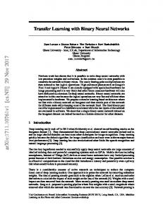
The performance of EBP algorithm has been evaluated in Soudry et al. (2014). However, those experiments are limited to high dimensional text datasets (the dimensions of the input feature vectors are from 11,463 to 238,739), and all the tasks are binary classification tasks. In this study, we will examine the performance of the EBP algorithm on image datasets for multiclass classification. To check the performance of EBP algorithm on deeper and small “fan-in” architectures on image classification, we use architectures with multiple layers and different hidden unites in experiments. Besides, we also explore the effectiveness of dropout techniques (Srivastava et al., 2014) in EBP algorithms. Two methods are used to input the image into the MNNs. The first method is to directly convert the 2D image into 1D vector by concatenating the pixels in the image in certain order, such as concatenating each row from top to bottom. For example, for the standard MNIST handwritten digits database, the input of each image is 28 × 28 vector. In the second method (spatial filtering method), we consider the spatial configuration of the images. The spatial configuration is considered in a similar way as Convolutional Neural Networks (CNN) (LeCun et al., 1998). Each unit in a layer receives inputs from a set of units located in a small neighborhood in the previous layer. As shown in Fig. 1, a unit in the feature map has 100 inputs connected to a 10 × 10 area in the input. Each unit has 100 inputs and therefore 100 trainable coefficients plus a trainable bias. Different from CNN, we only use one feature map in each hidden layer in this study.1 Since there is only one feature map, the network does not have the constraint that the connection weights for each unit in the feature map are the same. In the example shown in Fig. 1, there are 19 × 19 = 361 units in the second layer and each unit have (100 + 1) trainable weights. In implementation, the weight matrix between the first and second layer is set to 361×784. The weight matrix is initialized in the way that only the weights for connected units are nonzero, namely, 361 × 100 nonzero elements in the weight matrix. And the zero elements are kept zero during the whole training process. Because the EBP algorithm have the assumption of large fan-in, each unit in the hidden layers (feature maps) should be connected to a relative large neighborhood (such as “10 × 10” or larger) in the input layer. 1
The performance of EBP algorithm on standard CNN architectures will be studied in further work.
4
Algorithm 1 Expectation BackPropagation (EBP) algorithm for fully connected binary MNNs with binary synaptic weights and real bias (Soudry et al., 2014) . % νk,l = hvk,l i, tanh(hij,l ) = hWij,l i, and H is the set of all hij,l . Function [νL , Hnext ] = UpdateStepBinaryMNN(x, y, H) ⊲ Forward pass Initialize: ∀k : νk,0 = xk , ∀l : ν0,l = 1 for m = 1 → L do ∀k : P m−1 tanh(hkr,m )νr,m−1 ] µk,m = √ 1 [hk0,m + Vr=1 Km−1 P Vm−1 1 2 2 2 σk,m = Km−1 [(1 − νr,m−1 )(1 − δ1m ) + νr,m−1 sech2 (hkr,m )]] [1 + r=1 νk,m = 2φ(µk,m /σk,m ) − 1 end for ⊲ Backward pass Initialize: N (0|µi,L ,σ2 )
∆i,L = yi φ(yi µi,L )/σi,L i,L for l = L → 1 do PVm 1 2 N (0|µi,l−1 , σi,l−1 ) j=1 Kl−1 hij,l + √ 1 ∆i,l µj,l−1 Kl−1
∀i : ∆i,l−1 = √ ∀i, j :
hnext ij,l
=
tanh(hji,l )∆j,l
end for
10
19
10
10
19
10
28
output
28
Figure 1: A two-layer neural network architecture that considers the spatial context in images
4
E XPERIMENTS
In this section, we report the experiments of the EBP algorithm with MNNs with different architecture configurations in the standard MNIST handwritten digits database (LeCun et al., 1998). 4.1
E XPERIMENT S ETUP
The MNIST database contains 60,000 images (28 × 28 pixels) and the test set has other 10,000 images. During the training process, all the images in the training set were presented sequentially in each epoch with a randomized order. The task was to identify the label {0, 1, ..., 9}, using a BMNN classifier trained by EBP algorithm. The label is set to be yk = 2δk,label+1 + 1. We pre-process the training data by centralizing (mean = 0) and normalizing (std = 1) the pixels as recommended for BackPropagation (LeCun et al., 2012). As standard for classification with real values of MNNs. The output neuron with highest value indicates predicted label of the input pattern. 5
Method 1D Vector 2D Convolving
Table 1: Network architectures in experiments # of Hidden Layers # of Hidden Units One 200; 400; 600; 800; 1000 Two [200, 200]; [400, 400]; [600, 600]; [800, 800] One 144; 169; 196; 255; 256; 289 Two [361, 100]
When treating the image as 1D vector, a constant 1 is added to each input vector to allow some bias to the neurons in the hidden layer (so v0 = 785). For the spatial filtering method, a bias is added to each convolving block. Two neural network architectures are used: one hidden layer and two hidden layers. For each type of architecture, we vary the number of neurons in the hidden layers. The detailed configurations for the network architectures for both methods are shown in Table 1. In the spatial filtering method, different filtering block sizes are used in the one hidden layer architecture: 12×12, 13×13, 14×14, 15×15, 16×16 and 17×17. Thus, the corresponding hidden units are 289, 256, 255, 196, 169 and 144, which are the feature map size in the hidden layer. Taking block size 12 × 12 as an example, the feature map size becomes (28 − 12 + 1) × (28 − 12 + 1) = 17 × 17 = 289 hidden units. Accordingly, there are 12 × 12 = 144 inputs to each unit in the hidden layer, and 289 inputs to each unit in the output layer. We selected such configurations because of the large “fanin” assumption of the EBP algorithm. These configurations can also be used to learn whether it is better to set larger fan-in in the first layer or second layer. In the case of two-hidden-layer network, we only select one configuration because other configuration will lead to smaller fan-in (the hidden units [361, 100] correspond to 100 inputs to each unit in the first layer (10 × 10 block size in the input layer) and also 100 inputs (10 × 10 block size in the second layer) to each unit in the second hidden layer). We also employ dropout technique on all the architectures. Dropout is a technique for preventing overfitting and provides a way of approximately combining exponentially many different network architectures efficiently to improve performance (Srivastava et al., 2014). The effectiveness of dropout has been demonstrated on neural networks, DBN and DBM with traditional error backpropagation with stochastic gradient decent method (Srivastava et al., 2014). In this study, we investigate its effectiveness in the EBP algorithm. In the experiments, we fixed p = 0.8 for both hidden units and input units in all dropout nets. 4.2
E XPERIMENTAL R ESULTS
In the result presentation, we use four abbreviations for presentation simplicity: (1) B-EBP-D: Deterministic EBP (EBP-D, see Sect. 2.1) with binary weights; (2) B-EBP-P: Probabilistic EBP (EBP-P, see Sect. 2.1) with binary weights; (3) R-EBP-D: Deterministic EBP with real weights; and (4) R-EBP-P: Probabilistic EBP with real weights. All the results reported below are based on the networks trained by 120 epochs. Training with more epochs may improve the performances of some network architectures. For weight initialization, we used the same method as Soudry et al. (2014). Effects of Hidden Unite Number and Hidden Layer Number Table 2 shows the results of MNNs on MNIST dataset using EBP algorithms on different network structures without dropout. From the results, we can observe that for networks with one hidden layer, the increase of hidden units clearly improves the performance and the best performance is obtained with 800 units. Two-hidden-layer structure with EBP-P outperforms the one-hidden-layer structure significantly, even with only 200 hidden units in each layer. The results demonstrate the EBP works well on MNNs. Another observation is that EBP-P outperforms EBP-D, which is consistent with the results shown in Soudry et al. (2014). Particularly, the performance of B-EBP-D in the two-hidden-layer structure is worse than that of in the one-hidden-layer structure. With growing size of hidden units, performance of B-EBPD decreases quickly in two-hidden-layer models. We also use the EBP algorithm with real weights for all the configurations. The performances of EBP with real weights are better than the performance of EBP with binary weights in all structures. R-EBP-P in two-hidden-layer is only slightly better than in one-hidden-layer. Although R-EBP-D in two-hidden-layer performs worse than in one-hidden-layer as B-EBP-D, its performance increase when the number of hidden units increases. The standard BackProp algorithm (using tanh activation function and optimized learning rate) on 6
Table 2: Test errors without dropout for 1D vector method Hidden units
200
400
600
800
1000
[200, 200]
[400, 400]
[600, 600]
[800, 800]
B-EBP-P B-EBP-D
3.46% 4.63%
3.15% 3.89%
3.12% 3.62%
3.01% 3.63%
3.11% 3.57%
2.63% 5.20%
2.61% 5.91%
2.37% 13.51%
2.37% 27.06%
R-EBP-P R-EBP-D
2.78% 3.04%
2.29% 2.42%
2.28% 2.23%
2.20% 2.25%
2.25% 2.27%
2.16% 2.63%
2.22% 2.59%
2.22% 2.41%
2.10% 2.42%
Hidden units
200
400
600
800
1000
[200, 200]
[400, 400]
[600, 600]
[800, 800]
B-EBP-P B-EBP-D
3.60% 4.91%
2.82% 3.50%
2.82% 3.45%
2.55% 3.10%
2.52% 3.08%
2.93% 3.97%
2.39% 3.18%
2.12% 2.89%
2.12% 2.68%
R-EBP-P R-EBP-D
2.45% 2.58%
2.04% 2.09%
1.90% 1.94%
1.87% 1.91%
1.88% 1,86%
2.22% 2.51%
1.78% 1.99%
1.75% 1.87%
1.66% 1.75%
Table 3: Test errors with dropout for 1D vector method
the one-hidden-layer model with 800 units can obtain 2.13%2 , which is comparable for the best results obtained by R-EBP-P. Using binary weight will hurt the performance, while from the table, we can see that binary weights with optimal neural networks do not hurt the performance much (best performance of B-EBP-P is 2.37%, comparing to 2.10% of R-EBP-P). Effects of Dropout The results of EBP algorithms on different network structures with dropout are shown in Table 3. The results show the same observations as those of without dropout. Comparing the results between Table 2 and Table 3, we can see that using dropout can improve the performance in all configurations, which demonstrates that the dropout also works in the EBP algorithms. From the results of using 1000 units and 800 units in one-hidden-layer structure, we can see that without dropout, the result of 1000 hidden units is worse that that of 800 hidden units, while with dropout, the performance is continuously increasing when increase the hidden unit number from 800 to 1000. Besides, with dropout, the performance of B-EBP-D becomes reasonable. The results validate that dropout can effectively prevent overfitting in BMNNs with the EBP algorithm. Effects of Spatial Filtering Table 4 shows the results of MNNs using the EBP algorithm with the consideration of image spatial configuration. The best performance of spatial filtering method using binary weights is 3.56% (obtained by 225 hidden units in one-layer structure), which is worse than the results of using “1D Input Vector” method as shown in Table 2. On the contrary, the performances of using real weights can be improved by the spatial filtering method, as the performance is better than all the network structures using “1D Vector Input” method without dropout (the results in Table 2). The best results are obtained in the configuration of 256 hidden units (13 × 13 inputs to each unit in the hidden layer, and 256 inputs to each unit in the output layer). The results of this method shed light on the extension of the EBP method on Convolutional Neural Networks, such as the block size connecting to each unit in the feature map in each convolutional layer. Summary The analysis of experimental results gives us a few interesting findings. They include: (1) BMNNs with the EBP algorithm work well for image classification task, although the performance is not as good as real MNNs3 ; (2) even if the fan-in size is only few hundreds (e.g., [784, 200, 10]), the EBP algorithm still works well on BMNNs; (3) BMNNs with EBP-D algorithms on networks 2
Note that using error regularization and proper weight initialization, standard backpropagation can achieve better performance. For example, we can error rate by using L1 and L2 error regularization and q achieve 1.65% q 6 6 , ] with 500 hidden units. initializing the weight uniformly in [− f anin +f anout f anin +f anout 3
Note that the EBP algorithm on MNNs with real weight can obtain comparable results with respect to the standard BackPropagation method.
Table 4: Test errors without dropout for spatial filtering method Hidden units 144 169 196 225 266 289 [361, 100] B-EBP-P 4.06% 3.90% 3.87% 3.97% 4.07% 4.36% 4.96% B-EBP-D 4.31% 3.93% 3.73% 3.56% 3.93% 4.06% 4.87% R-EBP-P 2.51% 2.21% 2.07% 2.03% 1.87% 1.99% 1.93% R-EBP-D 2.82% 2.51% 2.18% 2.22% 2.17% 2.08% 2.02% 7
with two-hidden-layer (more layers) outperform the networks with one-hidden-layer; (4) dropout can significantly improve the performance of BMNNs with the EBP algorithm; and (5) BMNNs with the consideration of spatial filtering does not improve the classification performance, based on the results on MNIST.
5
C ONCLUSIONS
In this paper, we report the performance of binary multilayer neural networks (BMNNs) on image classification tasks. Expectation BackPropagation (EBP) algorithm is used to train BMNNs with different network architectures and the performance is evaluated on the standard MNIST digits dataset. Experimental results demonstrate that BMNNs with the EBP algorithm can achieve good performance on the MNIST classification tasks. The results also show that the dropout techniques can significant improve BMNNs with the EBP algorithm. Image spatial configuration improves the performance of networks with real weights but not that of BMNNs. In this study, we only conduct experiments on the MNIST dataset. The performance of BMNNs with EBP algorithm on image classification tasks needs to be further validated on other image datasets (e.g., CIFAR10). In the future, we would like to study the performance of standard Convolutional Neural Networks with the use of EBP algorithm and to explore different weight initialization methods. ACKNOWLEDGMENTS This is a course project for “Lab Course on Deep Learning (11-875)”, during Zhiyong Cheng’s visit to Carnegie Mellon University.
R EFERENCES Hinton, Geoffrey, Deng, Li, Yu, Dong, Dahl, George E, Mohamed, Abdel-rahman, Jaitly, Navdeep, Senior, Andrew, Vanhoucke, Vincent, Nguyen, Patrick, Sainath, Tara N, et al. Deep neural networks for acoustic modeling in speech recognition: The shared views of four research groups. Signal Processing Magazine, IEEE, 29(6):82–97, 2012. Karakiewicz, Rafal, Genov, Roman, and Cauwenberghs, Gert. 1.1 tmacs/mw fine-grained stochastic resonant charge-recycling array processor. Sensors Journal, IEEE, 12(4):785–792, 2012. Krizhevsky, Alex, Sutskever, Ilya, and Hinton, Geoffrey E. Imagenet classification with deep convolutional neural networks. In Pereira, F., Burges, C.J.C., Bottou, L., and Weinberger, K.Q. (eds.), Advances in Neural Information Processing Systems 25, pp. 1097–1105. Curran Associates, Inc., 2012. Lan, Zhen-Zhong, Jiang, Lu, Yu, Shoou-I, Rawat, Shourabh, Cai, Yang, Gao, Chenqiang, Xu, Shicheng, Shen, Haoquan, Li, Xuanchong, Wang, Yipei, et al. Cmu-informedia at TRECVID 2013 multimedia event detection. In TRECVID 2013 Workshop, volume 1, pp. 5, 2013. LeCun, Yann, Bottou, L´eon, Bengio, Yoshua, and Haffner, Patrick. Gradient-based learning applied to document recognition. Proceedings of the IEEE, 86(11):2278–2324, 1998. LeCun, Yann A, Bottou, L´eon, Orr, Genevieve B, and M¨uller, Klaus-Robert. Efficient backprop. In Neural networks: Tricks of the trade, pp. 9–48. Springer, 2012. Ribeiro, Fabiano and Opper, Manfred. Expectation propagation with factorizing distributions: A gaussian approximation and performance results for simple models. Neural computation, 23(4):1047–1069, 2011. Soudry, Daniel, Hubara, Itay, and Meir, Ron. Expectation backpropagation: parameter-free training of multilayer neural networks with continuous or discrete weights. In Proc. of NIPS, 2014. Srivastava, Nitish, Hinton, Geoffrey, Krizhevsky, Alex, Sutskever, Ilya, and Salakhutdinov, Ruslan. Dropout: A simple way to prevent neural networks from overfitting. The Journal of Machine Learning Research, 15 (1):1929–1958, 2014. Szegedy, Christian, Liu, Wei, Jia, Yangqing, Sermanet, Pierre, Reed, Scott, Anguelov, Dragomir, Erhan, Dumitru, Vanhoucke, Vincent, and Rabinovich, Andrew. Going deeper with convolutions. arXiv preprint arXiv:1409.4842, 2014.
8