1
A Quantum Multilayer Self Organizing Neural Network For Binary Object Extraction From A Noisy Perspective Siddhartha Bhattacharyya, Pankaj Pal and Sandip Bhowmick Department of Information Technology RCC Institute of Information Technology, Canal South Road, Beliaghata, Kolkata - 700 015 Email:
[email protected]; pal pankaj
[email protected];
[email protected]
Abstract Binary object extraction from a noisy perspective is a challenging proposition in the computer vision community. Various research initiatives based on different methodologies have been entrusted on this aspect over the decades. The multilayer self organizing neural network (MLSONN) architecture implemented by a fuzzy measure guided backpropagation of errors is one of the best accomplishment in this direction. In this article, a quantum multilayer self organizing neural network (QMLSONN) architecture is proposed to achieve the same objective. Quantum computation plays a remarkable role in the proposed architecture. The proposed architecture operates using single qubit rotation gates. Here different nodes and interconnection weights act as vital components for this intention. The proposed QMLSONN architecture comprises three processing layers specified as input, hidden and output layers. The nodes in the processing layers are represented by qubits and the interconnection weights are represented by quantum gates. A quantum measurement at the output layer destroys the quantum states of the processed information thereby inducing assimilation of linear indices of fuzziness as the network system errors used to adjust network interconnection weights through a proposed quantum backpropagation algorithm. Results of application of the QMLSONN are established on a synthetic and a real life spanner image with various degrees of Gaussian noise and uniform noise. Comparative study with the classical MLSONN architecture reveals the time efficiency of the presented QMLSONN architecture. Moreover, the QMLSONN architecture also restores the shape of the extracted objects to a great extent. Index Terms Multilayer self organizing neural network, binary object extraction, quantum computing, quantum backpropagation algorithm, quantum multilayer self organizing neural network
I. I NTRODUCTION
organizing neural network architectures have been used for object extraction and pattern recognition. Several neighborhood According to the computer vision research community, based network architectures like the multilayer self organizing accurate extraction of binary objects from a noisy background neural network (MLSONN) [14] are used for similar jobs. The is a challenging proposition. Several research initiatives have fundamental loom is centered on employing a fully connected been invested on this aspect over the decades. multilayer network architecture with each neuron of one layer Neural networks have often been employed by researchers connected to its neighboring neurons in the previous layer. for dealing with the tasks of extraction [1], [2], [3], classiSuch a network architecture, upon stabilization leads to the fication [4], [5], [6] of pertinent object specific information detection and extraction of objects by ways of self supervision from redundant image information bases and identification and of inputs. The MLSONN [14] architecture is a feedforward recognition of binary objects from an image scene [7], [8], [9]. network architecture and resorts to some fuzzy measures of Several neural network architectures, both self-supervised and the image information so as to derive the system errors. unsupervised, are reported in the literature, which have been Quantum Computation has evolved from the theoretical studies evolved to produce outputs in real time. of Feynman (1982), Deutsch (1985), and others, to an intensive Kohonen’s self-organizing feature map [10] is centered on research field since the innovation of a quantum algorithm, preserving the topology in the input data by subjecting the which can solve the problem of factorizing a large integer in output data units to assured neighborhood constraints. The polynomial time by Shor (1994). Matsui et al. [15] projected a Hopfield’s network [11] proposed in 1982, is a fully connected Qubit Neuron Model which exhibits quantum learning abilities. network architecture with capabilities of auto-relationship. A This model resulted on a quantum multi-layer feed forward photonic execution of the Hopfield network is also reported neural network proposal [16] which implements Quantum in [12], where a winner-take-all algorithm is used to imitate Mechanics (QM) effects, having its learning efficiency proved the state transitions of the network. on non-linear controlling problems [17]. Aytekin et al. [18] Numerous attempts have also been reported [13] where self
2
proposed an automatic object extraction procedure based on the quantum mechanical principles. Matsui et al. [15] anticipated a Qubit Neuron Model which exhibits quantum learning abilities. Ezhov [19] proposed a new model of quantum neural network to solve classification problems. It is based on the extension of the model of quantum associative memory and also utilizes Everetts principle of quantum mechanics. Quantum entanglement is liable for the associations between input and output patterns in the proposed architecture. In the field of artificial neural networks (ANN), some pioneers introduced quantum computation into analogous discussion such as quantum associative memory, parallel learning and empirical analysis [20], [21], [22], [23]. They constructed the establishment for further study of quantum computation in artificial neural networks. Menneer developed her Ph. D. thesis in which deeply discussed the application of quantum theory to ANN and established that QANNs are more efficient than ANNs for classification tasks [24]. Ventura and Martinez developed a quantum associative memory, its structure and learning manner in quantum version [25]. Weigang tried to develop a parallel-SOM and mentioned the once learning manner in quantum computing environment [26]. He also proposed an Entanglement Neural Networks (ENN) on the base of the quantum teleportation and its extension with smart sense. In AI and quantum computing, there is more recent review from Hirsh et al. [27], [28], [29], [30]. According to Perus, quantum wave function collapse “is very similar to neuronal-pattern-reconstruction from memory. In memory, there is a superposition of many stored patterns. One of them is selectively brought forward from the background if an external incentive triggers such a reconstruction” [31], [32]. A quantum neural computer consists of an ANN where quantum processes are supported. The ANN is a self-organizing type that becomes a different measuring system based on associations triggered by an external or internally generated stimulus. [21]. A quantum learning system might acquire some form of intentionally, and begin the bridging of the physical/mental gap. Menneer and Narayanan (1995) have applied the multiple universes view from quantum theory to one-layer ANNs. In 1997, Lagaris et al., [33] developed Artificial Neural Networks for Solving Ordinary and Partial Differential Equations. The use of quantum parallelism is often connected with consideration of quantum system with massive dimension of state space. The applications described further are used with some other properties of quantum systems and they do not stipulate such enormous number of states. The term “image recognition” is used here for several broad class of problems [34]. Quantum computation uses microscopic quantum level effects to perform computational tasks and has created results that in some cases are exponentially faster than their classical counterparts. The unique characteristics of quantum theory may also be used to create a quantum associative memory with a capacity exponential in the number of neurons [25]. Quantum Artificial Neural Networks (QANNs) are more efficient than Classical Artificial Neural Networks (CLANNs) for classification tasks, in that the time required for training is much less for QANNs. (Menneer and
Narayanan, 1998). The repetition is not required by QANNs, since each component network learns only one pattern causing the training set to be learned more quickly. Perus reported this as a basis for Quantum Associate Networks [35]. Quantum systems can realize content addressable associative memory [36]. Hu [37] developed a research about Quantum computation via neural networks applied to image processing and pattern recognition. He proved that the error in measurement produced by quantum principle is half the error produced by a classical approach. II. Q UANTUM C OMPUTING F UNDAMENTALS Quantum Computing is concerned with creating computational devices based on the principles of quantum mechanics. It defines quantum mechanical operations like superposition, entanglement [38] on them. Superposition is the property of quantum mechanics. Due to the linear dynamics the linear combination of each possible solution in a quantum mechanical system is also a solution. Entanglement is the property which generally gives rise to non-local interaction among bipartite correlated states. These properties have some profound implications. Problems like large integer factorization which is one of the cornerstones of today’s digital security, is rendered solvable in reasonable amount of time by a quantum computer whereas it was practically impossible to track on a standard classical computer. A quantum computer would not just be a traditional computer built out of different parts, but a machine that would exploit the laws of quantum physics to perform certain information processing tasks in a spectacularly more efficient manner. One demonstration of this potential is that quantum computers would break the codes that protect our modern computing infrastructure the security of every Internet transaction would be broken if a quantum computer were to be built. This prospective has made quantum computing a national security concern. Yet at the same time, quantum computers will also revolutionize large parts of science in a more benevolent way. Simulating large quantum systems, something a quantum computer can easily do, is not practically possible on a traditional computer. From exhaustive simulations of biological molecules which will advance the health sciences, to aiding research into narrative materials for harvesting electricity from light, a quantum computer will likely be an fundamental tool for future progress in chemistry, physics, and engineering. A. Concept of Qubits The most basic element of Quantum Computer is a qubit. It is represented as a linear superposition of two eigenstates |0⟩ and |1⟩. It is represented as |ϕ⟩ = α|0⟩ + β|1⟩
(1)
where, α and β are the probability amplitudes subject to the normalization criteria |α|2 + |β|2 = 1
(2)
The fundamental operations on these qubits are represented as unitary operators in the Hilbert space. These unitary transformations can be used to appreciate various logic functions.
3
These are the basic quantum gates [16] and contain the quintessence of quantum computation. B. Single qubit rotation gate The single qubit rotation gate is defined as ] [ cos θ − sin θ R(θ) = sin θ cos θ This operates on a single qubit to renovate it to ] [ [ ] cos θ − sin θ cos ϕ0 × R(θ) = sin θ cos sin ϕ0 [ ] θ cos(θ + ϕ0 ) = sin(θ + ϕ0 ) C. Quantum Measurement
(3)
(4)
in superposed form to a specific state required. To accomplish multi-qubit measurement, a succession of single-qubit measurements in the defined basis are performed. Suppose, at initial, the system is in the state |ψ⟩, then the probability of finding the state ϕ will be |cϕ |2 . III. M ULTILAYER S ELF O RGANIZING N EURAL N ETWORK A RCHITECTURE (MLSONN) MLSONN [14] is a self-supervised architecture efficient in extracting binary objects from a noisy and blurred background. It comprises several layers, viz. the input layer, any number of hidden layers and an output layer for obtaining the final processed output. The interconnection strategy employed between the layers follows a second order neighborhood topology. The network is characterized by forward propagation of incident information and subsequent processing at the hidden layers and the output layer. The network system errors are calculated at the output layer using the linear indices of fuzziness of the intermediate outputs obtained. These errors are used to adjust the network interconnection weights through the standard backpropagation algorithm. These intermediate outputs are fed back to the input layer for further processing. This process is continued until the network errors stabilize. Details regarding the operation and dynamics of the network can be obtained in [14].
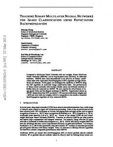
In quantum mechanics a system is described by its quantum state. In mathematical languages, all possible pure states of a system form a complete abstract vector space called Hilbert space, which is characteristically infinite-dimensional. A pure state is represented by a state vector (or precisely a ray) in the Hilbert space. In the experimental aspect, once a quantum system has been prepared in laboratory, some measurable quantities such as position and energy are measured. That is, the dynamic state of the system is already in an eigenstate of some measurable quantities which is probably not the quantity that will be measured. For pedagogic reasons, the measurement is usually assumed to be ideally perfect. Hence, IV. Q UANTUM M ULTILAYER S ELF O RGANIZING N EURAL the dynamic state of a system after measurement is assumed to N ETWORK A RCHITECTURE (QMLSONN) “collapse” into an eigenstate of the operator corresponding to the measurement. Repeating the same measurement without As QMLSONN is the quantum version of the MLSONN any significant evolution of the quantum state will lead to architecture [14], the processing nodes of the different layers the same result. If the preparation is continual, which does are simply qubits like not put the system into the previous eigenstate, subsequent measurements will likely lead to different result. That is, the ⟨α11 | ⟨α12 | ⟨α13 | . . . ⟨α1n | ... dynamic state collapses to different eigenstates. ... ... ... ... ... The values obtained after the measurement is in general ... ... ... ... described by a probability distribution, which is determined by ... ... ... ... ... an ”average” (or ”expectation”) of the measurement operator ⟨αm1 | ⟨αm2 | ⟨αm3 | . . . ⟨αmn | based on the quantum state of the prepared system. The probability distribution is either continuous (such as position and momentum) or discrete (such as spin), depending on ⟨β11 | ⟨β12 | ⟨β13 | . . . ⟨β1n | ... the quantity being measured. The measurement process is ... ... ... ... ... frequently considered as random and indeterministic. However, ... ... ... ... there is considerable dispute over this issue. In some interpreta ... ... ... ... ... tions of quantum mechanics, the result merely appears random ⟨βm1 | ⟨βm2 | ⟨βm3 | . . . ⟨βmn | and indeterministic, whereas in other interpretations the indeterminism is core and irreducible. A significant element in this disagreement is the issue of “collapse of the wave function” ⟨γ11 | ⟨γ12 | ⟨γ13 | . . . ⟨γ1n | ... associated with the change in state following measurement. ... ... ... ... ... In any case, our descriptions of dynamics involve probabilities ... ... ... ... and averages. For measurement purpose, we introduce the von ... ... ... ... ... Neumann measurement strategy which establishes one of a set ⟨γm1 | ⟨γm2 | ⟨γm3 | . . . ⟨γmn | of basis participating states as output. To continue this process, we first select a basis at random and ensure that the system The interconnection weights are in the form of rotation gates exists in the basis states. Quantum computing initiates some and also follow a second order neighborhood topology. A probabilistic measurement procedure that transforms the states schematic of the QMLSONN is shown in Figure 1.
4
Fig. 1. Schematic of a QMLSONN. Only few interconnections are shown for the sake of clarity.
A. Dynamics of operation When input data (inputi ) is given into the network, the input layer first converts the fuzzified input value [0, 1] into the phase [0, π2 ] in quantum states. yiI =
π (inputi ) 2
reversal parameter of j th hidden neuron. Similarly [39], uk =
m ∑
f (ψhqkoll )f (yjh ) − f (λk )
(12)
j=1
where, ψhqkoll are the connection weights between hidden and output layer and λk is the threshold of k th output neuron. I Here, (inputi ) are general inputs and yi are quantum inputs. Thus [39], Since we have input neurons i = 1 to l and hidden neurons j m m ∑ ∑ h = 1 to m, so [39] uk = eiψhqkoll eiyj − eiλk = ei (ψhqkoll + yjh ) − eiλk uhj
=
l ∑
(5)
j=1
f (ψipjhll )f (yiI )
−
f (λhj )
(6)
i=1
where, ψipjhll are the connection weights between input and hidden layer and λhj is the threshold of j th hidden neuron. From equation 6, we get [39], uhj =
l ∑
f (ψipjhll )f (yiI ) − f (λhj ) =
i=1
l ∑
I
h
eiψipjhll +yi )−f (λj )
i=1
(7)
= cos(ψipjhll + yiI ) + isin(ψipjhll + yiI ) − cos(λhj ) − isin(λhj ) (8) Now, π yjh = g(δjh ) − arg(uhj ) (9) 2 ∑ sin(ψipjhll + yiI ) − sinλhj π h −1 = g(δj ) − tan ∑ (10) 2 cos(ψipjhll + yiI ) − cosλhj =
π g(δjh ) − tan−1 (zh ) 2
(11)
∑ sin(ψipjhll +yiI )−sinλh j . Here arg(uhj ) means where, zh = ∑ cos(ψ +y I )−cosλh ipjhll
i
j
the phase extracted from a complex number u and δjh is the
j=1
(13) = cos(ψhqkoll +yjh )+isin(ψhqkoll +yjh )−cos(λk )−isin(λk ) (14) Now, π yk = g(δk ) − arg(uk ) (15) 2 where g(δk ) is the sigmoidal activation function. ∑ sin(ψhqkoll + yjh ) − sinλk π −1 = g(δk ) − tan ∑ (16) 2 cos(ψhqkoll + yjh ) − cosλk =
π g(δk ) − tan−1 (zk ) 2
(17)
∑ sin(ψhqkoll +yjh )−sinλk where, zk = ∑ cos(ψ . +y h )−cosλ hqkoll
j
k
In this way, the outputs are generated at the output layer of the QMLSONN architecture. A quantum measurement destroys the quantum states of the outputs at the output layer and convert the same to either 0 or 1 depending on a probability. However, since these outputs are to be further processed, these are retained in a safe custody. The probability amplitudes of the quantum states are compared with 1’s and 0’s using the linear indices of fuzziness to compute the system errors. These errors are used in a quantum backpropagation algorithm (to be discussed next) to regulate the interconnection weights of the network layers. The retained outputs are fed back to the input
5
layer for further processing. This process is repeated until the network system errors fall below a certain reasonable limit whence the object gets extracted from the noisy background.
Similarly, λnew = λold k k −η
∂E ∂λold k
(29)
Using chain rule, B. Quantum Backpropagation Algorithm
∂yjh ∂E ∂E In this section the quantum backpropagation error adjust= × (30) ∂ψipjhll ∂ψipjhll ∂yjh ment algorithm is discussed and generalized for any number of layers [40]. For this purpose, the probability amplitude of where, |0⟩ is attached to the real part and that of |1⟩ to the imaginary ∂E ∂yk part. = −(tn,p − outputn,p )[2sin(yk )cos(yk ) h ] (31) Two kinds of parameters exist in this neuron model: the phase ∂yjh ∂yj parameter of weight connection θ and threshold λ, and the reversal parameter δ. ∂E (tn,p − outputn,p )2sin(yk )cos(yk ) The network error is represented as = [ ] 1 + zk2 ∂yjh P N 1 ∑∑ cos(ψhqkoll + yjh )Re(uk ) Etotal = (tn,p − outputn,p )2 (18) [ ] 2 p n Re(uk )2 sin(ψhqkoll + yjh )Im(uk ) Here P is the number of learning patterns. tn,p is a target +[ ] (32) Re(uk )2 signal for the nth neuron and outputn,p means an outputn at the pth pattern. The error gradient is given by Now, ∂E ∂output ∂yjh 1 = tn,p − outputn,p (19) ] = −[ ∂θjk ∂θjk ∂ψipjhll 1 + zj2 ∂yk cos(ψipjhll + yiI )Re(uhj ) = −tn,p − outputn,p [2sin(yk )cos(yk ) ] (20) [ ] ∂ψhqkoll Re(uhj )2 1 ] = tn,p − outputn,p [2sin(yk )cos(yk ) 1 + zk2 cos(ψhqkoll + yjh )Re(uk ) + sin(ψhqkoll + yjh )Im(uk ) (21) Re(uk )2
=
+[
sin(ψipjhll + yiI )Im(uhj ) Re(uhj )2
∂E old ∂ψhqkoll
(22)
old new −η = ψipjhll ψipjhll
(23)
∂E π eiδk = (tn,p − outputn,p )[(2sin(yk )cos(yk ) ∂δk 2 (1 + eiδk )2 (24) Therefore, ∂E δknew = δkold − η old (25) ∂δk
∂yjh ∂λhj
= −[ [
1 ] 1 + (zh )2
cos(λhj )Re(uhj ) + sin(λhj )Im(uhj ) Re(uhj )2
]
(36)
Again, λnew = λold j j −η
∂E ∂output = (tn,p − outputn,p ) ] ∂λk ∂λk
(35)
where,
So, (26)
∂E ∂λold j
(37)
Using chain rule,
∂E δyk = (tn,p − outputn,p )(2sin(yk )cos(yk ) ∂λk δλk
(
(34)
∂yjh ∂E ∂E = × ∂λhj ∂yjh ∂λhj
∂E ∂yk = −[(tn,p − outputn,p )(2sin(yk )cos(yk ) ] ∂δk ∂δk
= −(tn,p − outputn,p )(2sin(yk )cos(yk )
∂E old ∂ψipjhll
Now, using chain rule, one gets,
where, η is the learning coefficient. So,
∂E ∂λk
(33)
Similarly,
Thus, the weight update equation takes the form new old ψhqkoll = ψhqkoll −η
]
(27)
1 1 + zk2
1 ))[cos(λk )Re(uk ) + sin(λk )Im(u(28) k )] Re(uk )2
∂yjh ∂E ∂E = × ∂δjh ∂yjh ∂δjh
(38)
π e−δj 2 (1 + δjh )2
(39)
where, ∂yjh ∂δjh
h
=
6
Fig. 2. Original images (a) Synthetic image (b) Real life Spanner image
V. E XPERIMENTAL R ESULTS
TABLE II C OMPARATIVE PERFORMANCE RESULTS OF QMLSONN
AND
MLSONN
ON THE TEST IMAGES AFFECTED WITH UNIFORM NOISE The application of the proposed QMLSONN has been established on a synthetic image and a real life spanner image QMLSONN MLSONN Synthetic image (Figure 2) affected with various degrees of Gaussian noise ϵ t(secs) pcc t(secs) pcc of zero mean and standard deviation of σ=8, 10 and 12 64% 3 99.9146 5 95.4285 and uniform noise with varied degrees ϵ=64%, 100%, 144%, 100% 3 99.5911 6 95.1294 196% and 256%. The noisy versions of the images are shown 144% 3 99.1455 7 94.1406 196% 4 98.3887 7 92.4927 in Figures 3 and 4. The same test images were considered 256% 8 96.2219 7 88.2690 with the conventional classical MLSONN architecture. The Real life image extracted Gaussian and uniform noise affected images with ϵ t(secs) pcc t(secs) pcc the MLSONN architecture are shown in Figures 5 and 6. The 64% 1 92.2974 2 89.1907 100% 2 92.2424 4 88.3972 respective extracted outputs obtained with the QMLSONN 144% 2 91.8518 5 87.2376 architecture are shown in Figure 7 and 8. From Figures 5, 6, 7 196% 4 90.5029 7 83.6548 and 8 it is evident that QMLSONN restores the shape of the 256% 6 87.3169 8 80.5969 objects much better after extraction. We have also computed the percentage of correct classification of pixels (pcc) [14] for the extracted images. In addition, we have also computed the VI. D ISCUSSIONS AND C ONCLUSION times of extraction for the two architectures. Table I lists the pcc values and the times of extraction (t) for the two images A quantum version of the MLSONN architecture is proobtained with the two architectures for the Gaussian noise. posed in this article. The architecture operates using qubits Table II lists the corresponding values for pcc and the times and rotation gates. The dynamics of operation of the proposed of extraction (t) for the two images for the uniform noise. It QMLSONN network and the corresponding quantum backis evident from Tables I and II that QMLSONN outperforms propagation is discussed. its classical counterpart as far as both the time complexity and The proposed QMLSONN network is found to outperform the quality of the extracted images. the classical MLSONN counterpart as regards to the time complexity as well as the extraction quality of the extraction process. Methods remain to investigate the application of the TABLE I C OMPARATIVE PERFORMANCE RESULTS OF QMLSONN AND MLSONN QMLSONN to the segmentation of multilevel images. The ON THE TEST IMAGES AFFECTED WITH G AUSSIAN NOISE authors are currently engaged in this direction.
QMLSONN Synthetic image σ t(secs) 8 12 10 15 12 21 14 39 16 40 Real life image σ t(secs) 8 12 10 18 12 19 14 37 16 67
MLSONN pcc 99.5361 98.7548 98.3093 97.0520 94.0917
t(secs) 63 63 65 68 92
pcc 91.5710 91.4550 91.2597 89.4409 83.9111
pcc 92.2851 91.9494 91.5344 90.6921 83.5815
t(secs) 44 42 41 67 94
pcc 85.3468 84.8937 84.5397 78.3386 73.3459
R EFERENCES [1] D. T. Pham and E. J. Bayro-Corrochano, “Neural computing for noise filtering, edge detection and signature extraction,” Journal of Systems Engineering, vol. 2, no. 2, pp. 666–670, 1998. [2] R. P. Lippmann, “An introduction to computing with neural nets,” IEEE ASSP Magazine, pp. 3–22, 1987. [3] S. Haykin, Neural networks: A comprehensive foundation, second edition, Prentice Hall, Upper Saddle River, NJ, 1999. [4] M. A. Abdallah, T. I. Samu, and W. A. Grisson, “Automatic target identification using neural networks,” SPIE Proceedings Intelligent Robots and Computer Vision XIV vol. 2588, pp. 556–565, 1995. [5] M. Antonucci, B. Tirozzi, N. D. Yarunin et al., “Numerical simulation of neural networks with translation and rotation invariant pattern recognition,” International Journal of Modern Physics B, vol. 8, no. 11–12, pp. 1529–1541, 1994.
7
Fig. 3. Gaussian noise affected images (a)(b)(c)(d)(e) Synthetic image at σ=8, 10, 12, 14 and 16; (a′ )(b′ )(c′ )(d′ )(e′ ) Real life Spanner image at σ=8, 10, 12, 14 and 16
[6] M. Egmont-Petersen, D. de Ridder, and H. Handels, “Image processing using neural networks - a review,” Pattern Recognition, vol. 35, no. 10, pp. 2279–2301, 2002.
[8] L. I. Perlovsky, W. H. Schoendor, B. J. Burdick et al., “Model-based neural network for target detection in SAR images,” IEEE Transactions on Image Processing, vol. 6, no. 1, pp. 203–216, 1997.
[7] B. Kamgar-Parsi, “Automatic target extraction in infrared images,” NRL Rev., pp. 143–146, 1995.
[9] P. D. Scott, S. S. Young, and N. M. Nasrabadi, “Object recognition using multilayer hopfield neural network,” IEEE Transactions on Image
8
Fig. 4. Uniform noise affected images (a)(b)(c)(d)(e) Synthetic image at ϵ=64%, 100%, 144%, 196% and 256%; (a′ )(b′ )(c′ )(d′ )(e′ ) Real life Spanner image at ϵ=64%, 100%, 144%, 196% and 256%
Processing, vol. 6, no. 3, pp. 357–372, 1997. [10] T. Kohonen, Self-organization and associative memory, Springer-Verlag, London, 1984. [11] J. J. Hopfield, “Neurons with graded response have collective compu-
tational properties like those of two state neurons,” Proceedings of Nat. Acad. Sci. U. S. pp. 3088–3092, 1984. [12] S. Munshi, S. Bhattacharyya, and A. K. Datta, “Photonic Implementation of Hopfield Neural Network for associative pattern recognition,”
9
Fig. 5. Extracted Gaussian noise affected images using MLSONN (a)(b)(c)(d)(e) Synthetic image at σ=8, 10, 12, 14 and 16; (a′ )(b′ )(c′ )(d′ )(e′ ) Real life Spanner image at σ=8, 10, 12, 14 and 16
Proceedings of SPIE, vol. 4417, pp. 558–562, 2001. [13] S. Bhattacharyya and U. Maulik, Soft Computing For Image And Multimedia Data Processing, Springer, Germany, 2013. [14] A. Ghosh, N. R. Pal, and S. K. Pal, “Self organization for object extraction using a multilayer neural network and fuzziness measures,” IEEE Transactions on Fuzzy Systems, vol. 1, no.1, pp. 54–68, 1993. [15] N. Matsui, M. Takai, and H. Nishimura, “A network model based on qubit-like neuron corresponding to quantum circuit,” The Institute of Electronics Information and Communications in Japan (Part III: Fundamental Electronic Science), vol. 83, no. 10, pp. 67–73, 2000. [16] N. Kouda, N. Matsui, and H. Nishimura, “A multilayered feedforward network based on qubit neuron model,” Systems and Computers in Japan, vol. 35, no. 13, pp. 43–51, 2004. [17] N. Kouda, N. Matsui, H. Nishimura, and F. Peper, “An examination of qubit neural network in controlling an inverted pendulum,” Neural Processing Letters, vol. 22, no. 3, pp. 277–290, 2005. [18] C. Aytekin, S. Kiranyaz, and M. Gabbouj, “Quantum Mechanics in Computer Vision: Automatic Object Extraction,” Proc. ICIP 2013, pp.
2489–2493, 2013. [19] A. A. Ezhov, (eds. Sameer Singh, Nabeel Murshed and Walter Kropatsch), “Pattern Recognition with Quantum Neural Networks,” in: Advances in Pattern Recognition ICAPR 2001, Springer Berlin Heidelberg, vol. 2013, pp. 60–71, 2001. [20] R. Chrisley, “Quantum learning, (eds. P. Pylkknen and P. Pylkk) “New directions in cognitive science,” Proceedings of the international symposium, Saariselka, pp. 77–89, Lapland, Finland, Helsinki. Finnish Association of Artificial Intelligence, 1995. [21] S. Kak, “Quantum Neural Computing,” Advances in Imaging and Electron Physics, vol. 94, pp. 259–313, 1995. [22] T. Menneer A. and Narayanan, “Quantum-inspired Neural Networks,” technical report R329, Department of Computer Science, University of Exeter, Exeter, United Kingdom, 1995. [23] E. C. Behrman, J. Niemel, J. E. Steck and S. R. Skinner, “A Quantum Dot Neural Network,” IEEE Transactions on Neural Networks, 1996. [24] T. Menneer, “Quantum Artificial Neural Networks,” Ph. D. thesis of The University of Exeter, UK, May, 1998.
10
Fig. 6. Extracted uniform noise affected images using MLSONN (a)(b)(c)(d)(e) Synthetic image at ϵ=64%, 100%, 144%, 196% and 256%; (a′ )(b′ )(c′ )(d′ )(e′ ) Real life Spanner image at ϵ=64%, 100%, 144%, 196% and 256%
[25] D. Ventura and T. Martinez, “Quantum Associative Memory,” IEEE Transactions on Neural Networks, 1998. [26] L. Weigang, “A study of parallel Self-Organizing Map,” e-print: http://xxx. lanl.gov/quant-ph/9808025, 1998. [27] H. Hirsh, “A Quantum leap for AI,” IEEE Intelligent System, pp. 9, July/August, 1999. [28] T. Hogg, “Quantum Search Heuristics,” IEEE Intelligent System, pp. 12– 14, July/August, 1999. [29] S. Kak, “Quantum Computing and AI,” IEEE Intelligent System, pp. 9–11, July/August, 1999. [30] D. Ventura, “Quantum Computational intelligence: Answers and Questions,” IEEE Intelligent System, pp. 14–16, July/August, 1999. [31] M. Perus, “Mind: neural computing plus quantum consciousness,” in Mind Versus Computer, Edited by M. Gams, M. Paprzychi and X. Wu, by IOS press, pp. 156–170, 1997. [32] M. Perus, “Common mathematical foundations of neural and quantum informatics,” in Zeitschrift Fur Angewandte Mathematik und Mechanik, vol. 78, no. 1, pp. 23–26, 1998. [33] I. E. Lagaris, A. Likas and D. I. Fotiadis “Artificial Neural Network
Methods in Quantum Mechanics,” Comput.Phys. Commun. vol. 104, pp. 1–14,l 1997. [34] A. Y. Vlasov, “Quantum Computations and Images Recognition,” e-print: http://xxx. lanl.gov/quant-ph/ 9703010, 1997. [35] M. Perus, “Neural Networks as a basis for Quantum Associate Networks,” in Neural Network World, vol. 10, no. 6, pp. 1001–1013, 2000. [36] M. Perus and Dey, “Quantum system can realize content addressable associative memory,” in Applied Mathematics Letters, vol. 13, no. 8, pp.31–36, Pergamon, 2000. [37] Z. Z. Hu, “Quantum computation via Neural Networks applied to Image processing and pattern recognition,” PhD thesis at the University of Western Sydney, Australia. [38] D. Ventura and T. Martinez, “An artificial neuron with quantum mechanical properties,” Proc. Intl. Conf. Artificial Neural Networks and Genetic Algorithms, pp. 482–485, 1997. [39] S. Bhattacharyya, P. Pal and S. Bhowmik, “A Quantum Multilayer Self Organizing Neural Network For Object Extraction From A noisy Background,” Proc. Fourth International Conference on Communication Systems and Network Technologies, pp. 512–518, 2014.
11
Fig. 7. Extracted Gaussian noise affected images using QMLSONN (a)(b)(c)(d)(e) Synthetic image at σ=8, 10, 12, 14 and 16; (a′ )(b′ )(c′ )(d′ )(e′ ) Real life Spanner image at σ=8, 10, 12, 14 and 16
[40] S. Bhattacharjee, S. Bhattacharyya, and N. K. Mondal, (eds. S. Bhattacharyya and P. Dutta), “Quantum Backpropagation Neural Network Approach for Modeling of Phenol Adsorption from Aqueous Solution by Orange Peel Ash,” Handbook of Research on Computational Intelligence for Engineering, Science and Business, pp. 649–671, 2012.
12
Fig. 8. Extracted uniform noise affected images using QMLSONN (a)(b)(c)(d)(e) Synthetic image at ϵ=64%, 100%, 144%, 196% and 256%; (a′ )(b′ )(c′ )(d′ )(e′ ) Real life Spanner image at ϵ=64%, 100%, 144%, 196% and 256%
13
Dr. Siddhartha Bhattacharyya did his Bachelors in Physics, Bachelors in Optics and Optoelectronics and Masters in Optics and Optoelectronics from University of Calcutta, India in 1995, 1998 and 2000 respectively. He completed PhD in Computer Science and Engineering from Jadavpur University, India in 2008. He is the recipient of the University Gold Medal from the University of Calcutta for his Masters. He is currently an Associate Professor and Head of Information Technology of RCC Institute of Information Technology, Kolkata, India. In addition, he is serving as the Dean of Research and Development of the institute from November 2013. Prior to this, he was an Assistant Professor in Computer Science and Information Technology of University Institute of Technology, The University of Burdwan, India from 2005-2011. He was a Lecturer in Information Technology of Kalyani Government Engineering College, India during 2001-2005. He is a coauthor of a book for undergraduate engineering students of WBUT and about 108 research publications international journals and conference proceedings.
He was the convener of the AICTE-IEEE National Conference on Computing and Communication Systems (CoCoSys-09) in 2009. He is the co-editor of the Handbook of Research on Computational Intelligence for Engineering, Science and Business; Publisher: IGI Global, Hershey, USA. He is the coauthor of the book titled ”Soft Computing for Image and Multimedia Data Processing”; Publisher: Springer-Verlag, Germany. He was the member of the Young Researchers’ Committee of the WSC 2008 Online World Conference on Soft Computing in Industrial Applications. He has been the member of the organizing and technical program committees of several national and international conferences. He is the Associate Editor of International Journal of Pattern Recognition Research. He is the member of the editorial board of International Journal of Engineering, Science and Technology and the member of the editorial advisory board of HETC Journal of Computer Engineering and Applications. He is the Associate Editor of the International Journal of BioInfo Soft Computing since 2013. He is the Editor-in-Chief of International Journal of Ambient Computing and Intelligence; Publisher: IGI Global, Hershey, USA. His research interests include soft computing, pattern recognition and quantum computing. Dr. Bhattacharyya is a senior member of IEEE. He is a member of ACM, IRSS and IAENG. He is a life member of OSI and ISTE, India.
Mr. Pankaj Pal did his Bachelors Degree in Science in 1990 from University of Calcutta, W.B., India, AMIE (Equivalent to B.Tech.) in Electronics and Communication Engineering in 1999 from The Institution of Engineers, India, and Masters in Information Technology in 2007 from Bengal Engineering and Science University, Shibpur, W.B., India. He is now working in PhD in the field of Soft Computing and Quantum Computing . He is currently an Assistant Professor of Information Technology of RCC Institute of Information Technology, Kolkata, India. Prior to this, he was an Instructor in the department of Electronics, of RCC Institute of Information Technology, Kolkata, India from 2002-2008. He was a Visiting Lecturer/Instructor in the department of Electronics of Kalyani Government Engineering College, Kalyani, Nadia, W. B., India during 19992002 and also was a Visiting Lecturer in the Jnan Chandra Ghosh Polytechnic ,Kolkata, India from 2000-2002. He was a Lecturer in The Institute of Modern Studies , Sodpur, 24-Pgs (N), W. B., India from 1994-2001. He is a co-author of research publications in international journals and conference proceedings. He was the member of The Institution of Engineers (India) since 2010. He is a Chartered Engineer (India), since 2011. His research interests include soft computing and quantum computing.
Mr. Sandip Bhowmick did his Bachelors in Commerce from University of Calcutta and Master of Computer Application and Master of Technology from West Bengal University of Technology, India in 2004, 2011 and 2014 respectively. He is currently a lab assistant of Techno India Hooghly College, Dharampur, Shantiniketan Near Khadina More, Chinsura 712101, India. He is a co-author of a paper in an International Conference.