Index Termsâfeature extraction, sensor data abstraction, event classification ..... plemented in Python, using publicly available library packages available from the ..... recognition (for ecg-based sensing),â in 5th International Conference.
Trainspotting: Combining Fast Features to Enable Detection on Resource-constrained Sensing Devices Eugen Berlin and Kristof Van Laerhoven
I. I NTRODUCTION Deploying a sensor network offers various positive and welldocumented implications, such as minimizing the intrusion and disruption of the environment and its inhabitants, and being able to monitor wide areas with a minimum of resources. Wireless sensor network applications have traditionally focused a lot on the periodic sampling of sensor data over long stretches of time and space, by using robust, distributed, and powerefficient sensor devices that collectively observe phenomena from a variety of locations. Many sensor network applications observe trends over an area by regularly sampling slowmoving values such as humidity or air pressure, meaning that nodes periodically wake up and disseminate their information across the network. Another well-published type of application aims at spotting sporadic events, such as sudden rises in temperature or the presence of methane, which are tackled by detection on the individual nodes. The advantage of this type of sensing is that the nodes themselves already filter out most of the sensor data, creating less overhead for the wireless medium that is shared between nodes. Recent advances in computer technology, in hardware as well as in software, have lead wireless sensor networks to be more scalable with their nodes being deployable for longer periods of time and being able to achieve battery-preserving low-power modes. Sensor networks have also been deployed c 2012 IEEE 978-1-4673-1786-3/12/$31.00 �
variance
Abstract—This paper focuses on spotting and classifying complex and sporadic phenomena directly on a sensor node, whereby a relatively long sequence of sensor samples needs to be considered at a time. Using fast feature extraction from streaming data that can be implemented on the sensor nodes, we show that on-sensor event classification can be achieved. This approach is of particular interest for wireless sensor networks as it promises to reduce wireless traffic significantly, as only events need to be transmitted instead of potentially large chunks of inertial data. The presented approach characterizes the essence of an event’s signal by combining several simple features on lowcost MEMS inertial data. Using a scenario and real data from vibration signatures generated by passing trains, we show how with this approach the classification of passing trains is possible on miniature nodes placed near the railroad tracks. Experiments show that, at the cost of slightly more local processing, the chosen features produce good train type classification with up to 90% of trains correctly identified. Index Terms—feature extraction, sensor data abstraction, event classification, wireless sensor networks
acceleration
Department of Computer Science Technische Universit¨at Darmstadt {berlin,laerhoven}@ess.tu-darmstadt.de
Fig. 1. A small sensor placed directly at the railway tracks captures vibrations caused by passing trains. From the raw sensor data of these events (middle plot), features can be extracted that are characteristic enough to be be used for on-sensor event estimation and classification (bottom plot).
to monitor or detect critical events, such as geothermic activity [1] or emergency scenarios [2], [3], that require high-fidelity data analysis in (or close to) real-time. This often conflicts with the fact that wireless sensor networks are heavily constrained by their hardware resources. In particular wirelessly transmitting the raw sensor data to a base station that has the processing capabilities will require high amounts of energy, and this will often constitute the main reason that nodes in the network to run out of battery power. This paper focuses first and foremost on data abstraction in cases whereby sensors are sampled at relatively high frequencies, from hundreds of Hertz for inertial sensors up to thousands of Hertz for microphones. We argue that onnode data abstraction is still possible with a combination of simple features based on mean, RMS, standard deviation, or signal amplitude that can be computed on microcontrollerbased hardware. For events that need to be represented by thousands of samples onward, such characterization would pay of as it reduces the raw data to a fraction of its original size. Figure 1 depicts a typical event in the case study that was used in this paper to evaluate our approach: The vibrations caused by passing trains are captured nearby the railway tracks by a small sensor node that is equipped with a sensitive inertial sensor. From the sensor’s readings signature, we propose to extract a set of features that can be used for detecting what type of train just passed and to approximate what its length was in wagons. The features can be calculated in an online fashion, meaning that they can be implemented on sensor platforms where memory and storage resources are limited.
978-1-4673-1786-3/12/$31.00 ©2012 IEEE
The remainder of this paper is structured as follows: In section II we will frame this research amid the most important and relevant related work. Section III is dedicated to our feature extraction approach. The sensor hardware is explained in section IV. Our experimental dataset is being presented in section V, while the evaluation and the chosen parameters and the results will be presented in section VI. Finally, we will discuss our results in section VII. II. R ELATED W ORK Sensors to monitor infrastructure, such as roads, railways, buildings, bridges have featured in quite a few research scenarios to motivate wireless sensor network infrastructures. The diversity of type of applications, of the employed sensors, and of the deployment and setup procedures has grown hugely. Monitoring and anomaly detection in structures is highly sought after to improve safety and organize maintenance tasks. Event and flow detection for alarm systems or traffic management is another popular category of application scenario. This section highlights several application scenarios that are tangent to our case study of train detection, and presents other related work in sensors and features for event detection. Bridge health monitoring systems, such as in [4], use vibrations and apply independent component analysis (ICA) and other complex and computationally expensive features and approaches to monitor and ensure infrastructure safety. Several application scenarios have been proposed that also target railway safety and train detection. Train arrival detection with accelerometers, presented in [5], is used to set of an alarm to warn workers on tracks, being a short-term deployment scenario that uses off-the-shelf accelerometer and communication system. In [6], the need for train detection is motivated, presenting some established train detection systems (e.g. axle counters to count wagons) and giving an outlook on future systems such as ERTMS/ETCS or satellite-based ones. Vibration sensors on running trains are used in [7] to monitor rail deformation thus increasing safety. Another work, [8] presents a train wheel detection system based on electromagnetic sensor arrays. A wireless sensor network is presented in [9] that is aiming at monitoring railroad operation, reducing the number of accidents and improving the efficiency of maintenance activities. Various research, such as [10], [11], [12] or [13], describe different application scenarios to detect and classify rare events. They focus on distributed observation of an area to spot the presence of ground vehicles or humans using visionbased, acoustic, seismic, magnetic and infrared sensors. While the deployment scale of these scenarios differs a lot, the feature set is kept relatively simple in these works. This correlates with the need or desire of deploying especially low-power and low-computation sensors. In the research scenario of a car toll system [12], types of vehicles such motorcycles, cars, pickup trucks, vans, and buses, are detected using the vehicle length, average observed energy and hill-pattern peaks in the signal are chosen as features that are easy to compute, following a very similar approach to the one taken in this work.
Power efficiency is a big topic throughout the sensor network community, but also in other research domains. The power constraints also hold for instance in the wearable and mobile sensor research domains, leading to approaches that aim at processing more data at its source, instead of transmitting the sensor data to a base station or just storing it in local memory. Detecting activities on a smart phones a processing platform, as presented in [14], will reduce the communication load and extend the lifetime of the sensors. This paper focuses especially on those wireless sensor network applications that observe phenomena that cannot be detected trivially by for instance sensor values passing set thresholds. To this end, we chose the detection of train types by means of the vibration signature they exhibit in nearby inertial sensors. The events in this scenario are (1) happening sporadically with most of the time nothing happening, (2) short in nature as trains’ vibration patterns tend to take some seconds to maximally a few minutes, and (3) can be detected by many redundant sensors along the same track to ensure high-enough precision in detection. Detection of trains in the categories that will be given later would for instance enable giving workers on the railroad more information on typical train speeds, or would enable railroad bridge engineers to deduce an approximate figure on weight and usage of said structure. The next section will present the proposed features that in combination will give an abstract but sufficiently rich picture of the events so that they can be detected with straightforward classifiers. Though also the classifiers would perhaps be implementable on the nodes themselves, we focus on the feature extraction and investigate classifiers later in the evaluation. III. F EATURE E XTRACTION Focusing on the application of spotting and categorizing passing trains as a representative scenario for a wider range of application types, the main goal is to extract simple features directly on the sensor node itself, and propagate either these throughout the network instead of raw data or a classification based on these. In both cases the feature calculation is focused on, while we assume the classification to be either straightforward enough to also implement on the sensor node, or be done on a more powerful platform at the network’s sink. For the rest of the paper, including the experiment setup, we will assume a sensor sampling rate of 100Hz and the data resolution set to 10 bit. Although this is far from sufficient for exact vibration analysis, we argue that with using the basic features discussed in this section on data from lowcost but precise MEMS inertial sensors suffices to capture the events for the application’s needs. The features discussed here will thus not rely on calculations and transformations in the frequency domain but instead approximate shapes and amplitudes within the signal to enable event classification. Events are assumed to occur sparsely over the course of time, so most of the data acquired by the sensor is not relevant and can be discarded after verifying no events are present in the data. A windowed standard deviation calculation was found to accurately detect these flat signal sections between events.
Whenever an event occurs, the sensor node will thus detect the changing sensor values, including the start and stop times of the event and the event duration, and temporarily buffer the sensor data from the event for further evaluation. As the node’s RAM tends to be limited, storing of the data stream can be done in an online fashion on peripheral memory such as an attached SD card. The feature analysis and calculation are thus limited to online algorithms: They are required to run incrementally on partial buffers of the event’s data at a time. Since the sensor has the time of event occurrence and also its duration in number of samples, the latter can directly be used as a distinct feature. This feature is similar to what others have used to detect types of ground vehicles, for instance [12]. As we are interested in abstracting the vibrations pattern caused by trains, using the overall variance to describe a train event would be another higher-level feature. Extracting other features from the sensor data that describe the signal footprint requires a more detailed look at the signal properties. For this, the vibrations caused by each axle or carriage/truck of train wagons, can be extracted by a sliding window approach and represented as variance peaks, as shown in Figure 1. Counting these local maxima in the variance will create a feature that is expected to correlate to the number of wagons in the train. The amplitude of the signal was also chosen as a feature. Hereby, either the real signal amplitude can be utilized or alternatively, since the windowed variance is computed for the above described peak detection, the maximum peak value as a representative for the amplitude can be used instead (the latter is visible in the bottom plot of Figure 1). The ability to characterize the events directly on the sensor node with these features makes it possible to forward these few abstractions of the event instead of its original raw sensor data representation. When considering a wireless sensor network that should be deployed for railway monitoring tasks, this means a much more energy efficient way of notifying a base station or logging data for future offline analysis. The presented feature routines are in essence the result of a trade-off between having highly-accurate vibration information but requiring a high amount of processing power, and settling for more abstract information while being able to do these calculations on more light-weight platforms. The features also do not require thousands of samples per second. From this follows that relatively low-cost and low-power sensor nodes can be utilized with microcontrollers that can for instance lack floating point units, as the next section will specify. IV. S ENSOR H ARDWARE The type of sensor is critical to the experimental data described in the next section, in which trains’ vibration footprints were captured while passing by the deployed nodes. This section provides the implementation details on the design choices for this type of node, as deployment issues are in this scenario crucial. It argues in particular for the use of an inexpensive and power-efficient inertial sensor to detect and characterize trains passing by, rather than using more accurate but also more resource-demanding vibration sensors.
Fig. 2. The sensor node board with microcontroller, accelerometer and microSD card used for the collection of this paper’s dataset. The USB port was used for configuring, initiating logging for the sensor node and afterwards accessing the captured data. A weatherproof plastic enclosure holds all components including a small lithium-polymer battery (size: 37x33x15mm).
Since the sensor node needs to be surviving a longitudinal deployment at a train track, the targeted environment can be expected to be especially hostile. Even though the used sensor node is a research prototype, a plastic enclosure was used and practical considerations for deployability included a range of outdoor situations that might damage the sensor node: • extremely high and low temperatures caused by direct sunlight in summer or snow cover in winter • high amounts of humidity, snow or rain conditions • accumulating dust and presence of dirt • limited availability of a nearby power supply The sensor modules used in the evaluation for this paper’s were designed to be small, robust and inexpensive enough to be left at the tracks in a variety of weather conditions. Built around a Microchip PIC microcontroller, an SD card for local storage and a 3D MEMS accelerometer (Fig. 2), the sensor’s main board contains interfaces for reprogramming, wireless extension, configuring the sensor node, and additional sensors such as light or temperature sensors. The 3D ADXL345 accelerometer is set to sample its data at 100Hz and message the data in bursts of 32 samples to the microcontroller. The gaps between the bursts thus give the microcontroller enough time to process the previous burst of sensor data and to go into a low-power idle mode to preserve battery power. The sensor was configured for sensing vibrations on its most sensitive setting, using the low ±2g range and the full 10-bit resolution. The node’s battery is a small-scale 180mAh lithium polymer battery which is able to power the sensor for approximately two weeks while logging all data to the SD card. The choice of low-power microcontroller-centered design makes the entire module small and cheap to produce, but also brings one of the bigger challenges that this paper faces: The limited amount of memory resources and the lack of a floatingpoint unit poses a harsh limit on the used algorithms and their implementation. The proposed feature routines therefore need to be able to work under strict memory constraints and should avoid the use of complex functions as they are for example used in Fourier analysis, as discussed in the previous section.
Fig. 3. Different train types that were recorded and classified during the evaluation. Fast inter-city and the city hopper passenger trains at the top, a fast regional passenger train in the middle, and a cargo train at the bottom.
The choice for an inexpensive off-the-shelf MEMS inertial sensor to detect and characterize particular trains by the vibrations they generate, has two consequences: (1) These sensor nodes could be built easily in large quantities, while occupying a minimal volume and generating data at a bandwidth and resolution that can be immediately processed by the on-board available processing power. (2) On the other hand, the quality of the sensor data can be expected to be less accurate than that of specifically-designed vibration sensors, placing more importance on the extraction of distinctive and characteristic features as proposed in this paper. The raw logging used only about 20% of program and random access memory. The proposed feature calculations would thus comfortably fit on these sensor nodes, enabling execution in an online fashion on the sensor node to forward only these through the wireless network instead of the usually larger amount of raw vibration data. To evaluate whether the features are descriptive and discriminant enough, however, we will in the remainder of this paper perform an experiment on their quality in characterizing observed vibration patterns. The following section will describe the deployment of the sensor nodes and the type of events that were captured in the datasets. V. T RAINSPOTTING DATASET The experiments discussed in this paper rely on a dataset taken with the prototype sensor node, discussed in the previous section, while placed nearby a railroad track. This section presents the recorded dataset and gives an overview on its characteristics and information content. The data used in this paper comes from two separate recordings that were conducted nearby two different railroad tracks in different locations, in order to have an as rich as
Fig. 4. Part of the data set, showing approximately 35 hours of sensor data (top plot): The data contain sparse but complex events caused by passing trains. Vibrations patterns shown in the two bottom plots were caused by a regional passenger train accelerating from the nearby station (duration 16 seconds) and a cargo train with loaded wagons (duration 30 seconds). The proposed features were tested on this data with two common classifiers.
possible dataset. The combined data contains in total 247 events, where an event is defined as a train passing by, whereby 182 of the trains were annotated with the corresponding train type as they could be traced by to the available train schedule. The remaining 65 train events were labeled with ”unknown” and not used in the classification evaluation. Figure 3 shows some types of trains that were observed to be running on those tracks. Figure 4 shows this part of the dataset, including a zoom-in on a fraction of the data, and showing two exemplar events caused by a regional passenger train and a cargo train. The first of the two recordings comes from a low duty railroad track and has approximately 24 hours of continuous sensor data, during which in total 53 trains passed by. This track services only smaller passenger trains that consist of a two-car articulated unit (Fig. 3, upper right). At certain times during the day, mostly during rush hours, there are also trains running that consist of multiple such wagons. The sensor’s location was not nearby a station or place where trains tend to slow down. The trains’ signatures thus tended to be relatively short and passing by at similar speeds. The second recording was added to the first to increase the dataset’s complexity by having been carried out on a busier railroad, spanning 35 hours of continuous data collection and capturing 194 train events in total. This track is used by a higher variety of trains, such as inter-city and regional passenger trains as well as cargo trains. The sensor node was this time also deployed nearby a train station that is only served by some regional passenger trains. While some passenger trains as well as cargo trains were passing the train station without slowing down at the station, others did decelerate and accelerate from this station, thus adding more diversity to train speeds and thus their signature’s length.
Being interested in the 182 labeled events only, the rest of the data was discarded as irrelevant for this kind of application after verifying that all events were indeed from passing trains (and not for instance from other application-irrelevant events). In a wireless sensor network scenario, it would be a common approach to discard the data between events, i.e., the flat accelerometer signals between trains passing by, then process the raw data from events locally and only transmitting the result of the feature processing or classification. In the case of this paper’s study, results needed to be reproducible and we therefore opted for continuous logging of raw data on the local flash memory, which is also a power-intensive operation. Since the dataset contains many different train types that mainly differ by name due to their scheduled tours, but in reality turn out to be similar regarding the type of wagons and locomotive used, a decision was made to group the annotations in four main categories. The categories reflect main train types as they tend to be found on European railroads. The three intercity passenger train types (ICE, IC, EC) mostly consist of same type and number of wagons are therefore grouped as class A. The two regional train types (RE, RB) were categorized as class B. All types of cargo trains were put together in class C, while so-called city-hopper passenger trains form class D. After retrieving the nodes and downloading their recorded data, annotations were added by using available train schedules as well as train configuration databases that specify how the trains were constituted, including number of wagons and position of the locomotive(s). No further data was available regarding the cargo trains, and unscheduled or re-directed trains, some of which were single locomotives without wagons, that could not be traced back in the schedules were as previously mentioned disregarded. Figure 3 shows photos of different train types running on the rail tracks of interest. The first class consists of fast inter-city passenger trains that contained 5 up to 9 wagons. The second class are the fast regional passenger trains that consist of 5 to 8 wagons, whereby there are some trains that stop at the nearby train station while others do not. The city hopper passenger trains consist of 2-car articulated units, whereby multiple such wagons are put together during rush hours. Finally, there is the cargo train class that had the most diverse setups and speeds, but mostly consisted of a much longer signature (due to having a bigger locomotive pulling far more wagons than the trains in the passenger train category). The next section will discuss the implementation and parametrization of the features used with this dataset to classify the train events present in this dataset, as well as the evaluation and discussion of the results. VI. E XPERIMENTS This section describes the offline evaluation of the previously presented features on the data set introduced in the previous section. First off, the parametrization details for the features and the methodology is given for the evaluation, followed by a discussion of the actual evaluation results.
A. Evaluation setup This section discusses which features have been extracted from sensor data with which set of parameters, and how they were evaluated by using them to classify the train events. Since our experiments were conducted offline for reproducibility, a first step requires that from the large amount of data only the actual train events are detected from sensor data. With this step we also acquire the start and stop time of an event, thus being able to compute its duration (in milliseconds). Additionally, the overall variance of this event is computed to give a rough estimation on how much vibration the train has caused. More specifically, valid patterns are detected by computing the variance over a sliding window with a relatively small size of one second (using half a second for window overlap) and a small threshold (set to 1.5 to cancel out the small amounts of noise in the original raw data). Start and stop boundaries of each event, along with its raw data and its duration, were extracted as separate data chunks for further analysis. For each of these events, the overall variance was added and used as a feature for classification. In addition to these overall event features, a more short-term sliding window was used to extract dense vibration patterns that correspond to the wheel impacts on the rails. For this step, the choice of window size is crucial, as from this depends whether we will be counting the axles, the trucks (also called ’bogie’ or a ’wheel truck’), adjacent trucks, or whole wagons (carriages with multiple axles). This truck count will then be used as another feature for classification, but might also be of interest to an application that requires tracking the train length or the train’s configuration (e.g., in rail bridge monitoring). To achieve this, we tested sliding window sizes on the interval from 100 up to 300 milliseconds (or 10 to 30 samples). Computing windowed variance resulted in the characteristic plots shown in Figure 5, with the raw sensor data is the upper and the resulting variance in the bottom plot. Hereby, a window size of 160 milliseconds was found to produce best classification performance. Using a peak detection algorithm based on the slope of the signal, the local maxima in the variance plot were found and highlighted as green dots. The number of peaks thus tends to correlate to the number of wagons the train consists of, and this feature can be expected to be of particular importance for distinguishing the cargo train class (an example of this can also be seen in Fig. 5a). With this optimal window size of 160 milliseconds, an early analysis showed that counting the trucks to estimate number of passenger carriages worked fairly robust. Counting trucks to estimate the number of wagons for the cargo trains on the other hand turned out to be more error-prone, most likely due to the high vibration levels caused by the cargo wagons and the high variance of different train speeds (due to cargo trains often passing the nearby station at low speeds, and also speed limits that are for instance imposed during the night time or at peak times). Counting pairs of trucks (holding up to two axles each) of adjacent wagons, on the other hand, can be distinguished more easily for all train types.
1000
1500
2000
2500
3000
0
200
400
600
800
1000
1200
1400
variance
500
variance
0
acceleration
2 : [ 1472. 33.05 19. ]
acceleration
3 : [ 3120. 707.61 55. ]
(a) A cargo train event of 31 seconds duration. The raw signal suggests that the train cars were loaded less in the first and more in the second part. Here, 55 peaks were detected and some missed, probably due to high noise level.
(b) A regional train of 6 wagons accelerating from nearby train station. High variance peaks in the beginning indicate the locomotive. The variance peaks with decreasing time gaps in between show the impact of each truck.
200
300
400
500
600
0
100
200
300
400
500
600
variance
100
variance
0
acceleration
1 : [ 536. 167.02 9. ]
acceleration
2 : [ 480. 489.97 7. ]
(c) A regional train of 6 wagons not stopping at the train station. The high variance at the end of the event indicates that this train is being pushed by a locomotive. The variance peaks capture pairs of trucks of adjacent wagons.
(d) A fast inter-city passenger train of 8 wagons (including the locomotive) passing at high speed. The fixed window size is too wide and can not capture each truck, but pairs of trucks of adjacent connected wagons.
100
150
200
250
0
100
200
300
400
500
variance
50
variance
0
acceleration
4 : [ 480. 46.98 6. ]
acceleration
4 : [ 264. 27.42 3. ]
(e) A city hopper passenger train is a 2-car articulated unit equiped with three trucks, two axles each. Reducing the sliding window size might allow capturing each axle separately.
(f) This city hopper passenger train consists of two wagons, thus having 6 trucks with 2 axles each. The variance peaks nicely correspond to the 6 trucks, having almost no gap between the two wagons.
Fig. 5. Examples of train events that were detected in the sensor data. Each subfigure shows raw acceleration data in the upper and variance computed on a sliding window of 0.16 seconds in the bottom plot. Peaks extracted from the variance are marked with green bullets. Due to various train assemblies as well as different train speeds, just counting the number of variance peaks computed on a fixed sliding window will not give a good classification performance.
With these features calculated, a 5-fold leave-one-out cross validation study was conducted. All events were grouped per train class and those were divided in 5 folds, whereby 4 were used for training the classifier and remaining fold was used for testing. For each fold, the true labels of the cross validation part (given by the annotation of the dataset) as well as the labels obtained by the classification were stored, and afterwards used to build the confusion matrices. From a confusion matrix, we then compute the classification accuracy per class of interest as well as the total accuracy for the given set of features and chosen parameters. Two classifiers were used for the evaluation: The K nearest neighbor (kNN) classifier was chosen particularly due to its simplicity and popularity. Additionally, a support vector machine (SVM) classifier was chosen for comparison. This way we are able to evaluate the features’ performance, and test whether the choice of the classifiers has a significant impact, too. For the kNN classifier, k was set to 5 nearest neighbors, as it was found to produce best classification results. In the SVM case, a linear kernel was used. The evaluation was implemented in Python, using publicly available library packages available from the Debian software repository, namely the mvpa library for the kNN and svmutil for the SVM.
B. Evaluation results This section presents and discusses the results of the kNN and SVM classifiers that were chosen for the evaluation. The confusion matrices given in Figure 6 show the classification performance for the kNN classifier and the four train categories. The confusion matrices for the SVM classifier are given in Figure 7. For these, the different sets of features were tested, while the best performing parametrization with 5 folds, k = 5, and the sliding window size of 0.16 seconds were set. Relying on the event duration as a single feature results in a weak classification performance, as can be seen in the confusion matrix shown in Figure 6a. The fast inter-city trains are mostly confused with the city hopper trains, reaching a class accuracy of only 22.22%. The reason for this strong confusion lies in the relation of speed and train length: on average a short and slow city hopper train generates a vibration pattern that is as long in time as the fast inter-city trains which are longer but pass by faster (from 3 up to 7 seconds). The same observation holds for other train types as well, whereby other train classes do not exhibit such high degree of confusion, reaching class accuracies of 61.76, 85.71 and 67.92% respectively. The regional passenger train class is being confused with all other train classes, probably because
4
1
B
4
21
5
11
66
C
D
13
B
13
A
11
5
4
B
8
26
C
1
1
D
2
36
4
A
(a) Event duration only
C
predicted class
D 2
75
51
(b) Event duration and variance
A
B
A
16
2
B
7
24
C
1
C
1
predicted class
D
2
76
actual class
A
predicted class
D
actual class
C
B
actual class
actual class
predicted class
A
53
D
C
A
B
A
9
7
2
B
4
26
4
4
C
D
4
(c) Duration, variance, # of peaks
D
73
3
46
(d) # of peaks only
Fig. 6. Summary of the kNN classification results for the train type classes (A to D) and different feature sets presented as confusion matrices: Combining all features results in the best performance. The classes are: A - fast inter-city trains; B - regional passenger trains; C - cargo trains; D - city hopper trains.
A
1
B
19
6
C
13
64
D
1
(a) Event duration only
predicted class
D
A
B
17
A
13
5
9
B
9
24
52
C
1
D
2
C
predicted class
D
1
76
51
(b) Event duration and variance
C
A
B
A
11
7
B
7
24
1
1
76
C
D
1
1
predicted class
D
2
51
(c) Duration, variance, # of peaks
C
A
B
6
4
8
B
25
9
C
3
A
actual class
C
actual class
actual class
B
actual class
predicted class
A
D
5
D
74
1
47
(d) # of peaks only
Fig. 7. Summary of SVM classification results for the train type classes (A to D) and features sets presented as individual confusion matrices. Event duration and variance are particular strong features. The classes are: A - fast inter-city trains; B - regional passenger trains; C - cargo trains; D - city hopper trains.
its many instances where they do not stop at the nearby train station (thus being as fast as inter-city trains at this particular spot) and trains that do and then accelerate from the station, leading confusion with long city hopper trains or very short cargo trains. The total accuracy for this feature and chosen classification parameters accounts to 69.78%. The SVM classifier’s performance with event duration as the single feature is much worse for the inter-city train class: these are heavily confused with the city hopper passenger trains (cf. Fig. 7a). The other classes perform considerably better, with 55.88, 83.12 and 98.11% per-class accuracy respectively, producing a total accuracy of 74.18%, and thus slightly outperforming the kNN classifier overall. Using the total event variance as a second feature significantly improves the kNN classification’s performance (Figure 6b). The accuracy for the inter-city class jumps to 61.11%, since the total vibration impact of a faster and heavier intercity train is higher than of the light city hopper, the confusion at this spot is drastically reduced compared to the previous results. A similar but less significant improvement can be observed with the cargo train and city hopper classes. The confusions between the inter-city and regional trains on the other hand still remains, which most likely is due to their similar duration and vibration signature. This especially becomes graspable when considering just the regional trains that
do not stop at the nearby train station and therefore do not slow down (cf. Fig. 5 c) and d)). All train type classes thus gain a performance boost, now reaching 76.47, 97.4 and 96.23% in per-class accuracy. The total accuracy for the chosen set of features lies at 89.56%. Only slightly better results can be achieved by the SVM classifier, where the total accuracy reaches 90.11% (Figure 7b). The number of peaks in the vibration pattern has been previously mentioned as an attractive feature candidate. Testing different window sizes from 0.1 up to 0.3 seconds in 0.02 steps revealed, to our surprise, that using the peaks as an additional feature does not improve the performance significantly. While there is no improvement for the kNN at all, the SVM classifier improvement accounts to 0.3 % over the previous feature set (with duration and overall variance). The reason might lie in the fact that the number of peaks corresponds heavily to the duration of the event already, and thus not offering much more information to distinguish train categories. Since the windowed variance was computed with a fixed window width for all events, regardless of their duration, one possibility to improve on the per-class accuracies might be to adapting the parameters for the windowed variance according to the length of the pattern. By adding the maximum value of the windowed variance (which represents the variance amplitude), we are able to boost the total accuracy a little
bit more, reaching 92.86%. When evaluating the performance of each class (Figure 6c), we observe that the city hopper train class is performing at 100% accuracy. Only one false hit happened with the cargo train class, being confused with a fast inter-city train. Some confusion still happens between the fast inter-city and the regional passenger train classes, which, as already mentioned, is most likely due to the non-stopping regional passenger trains that belong to the class. In this case, the kNN classifier shows better performance than the SVM, which reaches a total accuracy of 89.01%. When considering just the number of peaks (wagons, windowed variance footprint), without duration or total variance of the event, the classification performance drops to a total accuracy of 84.62% for kNN (Figure 6d) and 83.52% for SVM (Figure 7d). Since the number of peaks corresponds to the duration of the event on the one hand, but also covers the vibration properties of the trains, the obtained performance lies between the performances of duration on the one hand and duration with overall variance as features on the other. While the number of peaks did not improve the classification performance in our evaluation, the information encoded in this feature is still valuable. Using the number of peaks and the distances between those can be used to distinguish regional trains that are accelerating from the train station from the trains that do not stop there. Additionally, a feature pair consisting of the number of peaks together with the variance values might push the accuracy more, but is left for a planned further study over a larger data set. The comparison of the results for both chosen classification algorithms shows that the performance is very similar. While the classifications are comparable, the SVM approach requires much more time for training and evaluation. A lowfootprint version of the kNN classifier could furthermore be implemented on the sensor node, which could allow on-sensor classification with an overall accuracy over 90%. VII. C ONCLUSIONS This paper proposed a set of features for event detection in wireless sensor networks that can be calculated online on the individual sensor nodes, and are descriptive enough to allow characterization with a straightforward classifier. The features have as an advantage that only small descriptors need to be sent through the network, thereby reducing the network’s communication overhead and power demand. To evaluate the proposed features, a case study was presented in which small and robust wireless sensor nodes are deployed at train tracks to detect and identify passing trains by their vibration signature, as it is picked up by a sensitive inertial sensor on board. A real-world dataset was recorded, allowing a reproducible comparison of the proposed features and an evaluation on their impact on classification of events. It was found that with the event duration and overall variance the classification performance reaches a total accuracy of 89.56%. The best performing feature set consisted of the duration, the overall variance and the variance amplitude (value of the highest variance peak), reaching a total accuracy
of 92.86%. These results, achieved with a kNN classifier with k set to 5, performs similarly to an SVM classifier reaching a total accuracy of 92.31%, while being better suited for future explorations on on-sensor classification. At the time of writing, a larger-scale project is being started. We expect from this a significant gain of information that is needed for a long-term deployment of multiple sensors, as well as a throughout evaluation of our approach, with both offline as well as online classification implementations. This paper’s data set and evaluation scripts are available from the first author. R EFERENCES [1] G. Werner-Allen, K. Lorincz, M. Ruiz, O. Marcillo, J. Johnson, J. Lees, and M. Welsh, “Deploying a wireless sensor network on an active volcano,” Internet Computing, IEEE, vol. 10, no. 2, pp. 18–25, MarchApril 2006. [2] T. Gao, C. Pesto, L. Selavo, Y. Chen, J. G. Ko, J. H. Lim, A. Terzis, A. Watt, J. Jeng, B. rong Chen, K. Lorincz, and M. Welsh, “Wireless medical sensor networks in emergency response: Implementation and pilot results,” in 2008 IEEE Conference on Technologies for Homeland Security, December 2008, pp. 187–192. [3] T. Gao, T. Massey, L. Selavo, D. Crawford, B. rong Chen, K. Lorincz, V. Shnayder, L. Hauenstein, F. Dabiri, J. Jeng, A. Chanmugam, D. White, M. Sarrafzadeh, and M. Welsh, “The advanced health and disaster aid network: A light-weight wireless medical system for triage,” IEEE Transactions on Biomedical Circuits and Systems, vol. 1, no. 3, pp. 203–216, September 2007. [4] J. Huang, H. Ogai, C. Shao, J. Zheng, I. Maruyama, S. Nagata, and H. Inujima, “On vibration signal analysis in bridge health monitoring system by using independent component analysis,” in Proceedings of SICE Annual Conference 2010, August 2010, pp. 2122–2125. [5] L. Angrisani, D. Grillo, R. Moriello, and G. Filo, “Automatic detection of train arrival through an accelerometer,” in Instrumentation and Measurement Technology Conference (I2MTC), May 2010, pp. 898–902. [6] J. W. Palmer, “The need for train detection,” in IET Professional Development Course on Railway Signalling and Control Systems (RSCS 2010), June 2010, pp. 52–64. [7] C. Wang, Q. Xiao, H. Liang, X. Chen, X. Cai, and Y. Liu, “On-line vibration source detection of running trains based on acceleration measurement,” in 2006 IEEE/RSJ International Conference on Intelligent Robots and Systems, October 2006, pp. 4411–4416. [8] P. Donato, J. Urena, M. Mazo, J. Garcia, and F. Alvarez, “Electromagnetic sensor array for train wheel detection,” in Sensor Array and Multichannel Signal Processing Workshop Proceedings, July 2004, pp. 206–210. [9] E. Aboelela, W. Edberg, C. Papakonstantinou, and V. Vokkarane, “Wireless sensor network based model for secure railway operations,” in 25th IEEE International Performance, Computing, and Communications Conference (IPCCC 2006), April 2006, pp. 624–628. [10] S. Gupte, O. Masoud, R. Martin, and N. Papanikolopoulos, “Detection and classification of vehicles,” IEEE Transactions on Intelligent Transportation Systems, vol. 3, no. 1, pp. 37–47, March 2002. [11] G. P. Mazarakis and J. N. Avaritsiotis, “Vehicle classification in sensor networks using time-domain signal processing and neural networks,” Microprocess. Microsyst., vol. 31, pp. 381–392, September 2007. [Online]. Available: http://dl.acm.org/citation.cfm?id=1276528.1276723 [12] S. Keawkamnerd, J. Chinrungrueng, and C. Jaruchart, “Vehicle classification with low computation magnetic sensor,” in 8th International Conference on ITS Telecommunications (ITST 2008), October 2008, pp. 164–169. [13] P. Dutta, M. Grimmer, A. Arora, S. Bibyk, and D. Culler, “Design of a wireless sensor network platform for detecting rare, random, and ephemeral events,” in Proceedings of the 4th international symposium on Information processing in sensor networks, ser. IPSN ’05. Piscataway, NJ, USA: IEEE Press, 2005. [14] F.-T. Sun, C. Kuo, and M. Griss, “Pear: Power efficiency through activity recognition (for ecg-based sensing),” in 5th International Conference on Pervasive Computing Technologies for Healthcare (PervasiveHealth 2011), May 2011, pp. 115–122.