Apr 26, 2017 - Springer International Publishing, Cham (2014). 21. Uijlings, J.R.R., van de Sande, K.E.A., Gevers, T., Smeulders, A.W.M.: Selective Search for.
Relief R-CNN : Utilizing Convolutional Features for Fast Object Detection Guiying Li1 , Junlong Liu1 , Chunhui Jiang1 , Liangpeng Zhang1 , Minlong Lin2 , and Ke Tang1
arXiv:1601.06719v4 [cs.CV] 26 Apr 2017
1
School of Computer Science and Technology, University of Science and Technoloy of China, Hefei, Anhui 230027, P.R. China {lgy147,junlong,beethove,udars}@mail.ustc.edu.cn {ketang}@ustc.edu.cn 2 Tencent Company, Shenzhen, 518057, P.R. China {minlonglin}@tencent.com
Abstract. R-CNN style methods are sorts of the state-of-the-art object detection methods, which consist of region proposal generation and deep CNN classification. However, the proposal generation phase in this paradigm is usually time consuming, which would slow down the whole detection time in testing. This paper suggests that the value discrepancies among features in deep convolutional feature maps contain plenty of useful spatial information, and proposes a simple approach to extract the information for fast region proposal generation in testing. The proposed method, namely Relief R-CNN (R2 -CNN), adopts a novel region proposal generator in a trained R-CNN style model. The new generator directly generates proposals from convolutional features by some simple rules, thus resulting in a much faster proposal generation speed and a lower demand of computation resources. Empirical studies show that R2 -CNN could achieve the fastest detection speed with comparable accuracy among all the compared algorithms in testing. Keywords: Object Detection, R-CNN, CNN, Convolutional Features, Deep Learning, Deep Neural Networks
1
Introduction
One type of the state-of-the-art deep learning methods for object detection is R-CNN [8] and its derivative models [7,18]. R-CNN consists of two main stages: the categoryindependent region proposals generation and the proposal classification. The region proposals generation produces the rectangular Regions of Interest (RoIs) [7,18] that may contain object candidates. In the proposal classification stage, the generated RoIs are fed into a deep CNN [15], which will classify these RoIs as different categories or the background. However, R-CNN is time inefficient in testing, especially when running on hardwares with limited computing power like mobile phones. The time cost of R-CNN
2
G. Li et al.
comes from three parts: 1) the iterative RoIs generation process [12]; 2) the deep CNN with a huge computation requirement [15,22,10]; and 3) the naive combination of RoIs and the deep CNN [8]. Many attempts on these three parts have been made to speed up R-CNN in testing. For RoI generation, Faster R-CNN [18] trains a Region Proposal Network (RPN) to predict RoIs in images instead of traditional data-independent methods that iteratively generate RoIs from images like Objectness [1], Selective Search [21], EdgeBox [3] and Bing [2]. For the time consuming deep CNN, some practical approaches [9,14] have been proposed to simplify the CNN structure. For the combination of RoIs and the deep CNN, SPPnet [11] and Fast R-CNN [7], which are the most popular approaches, reconstruct the combination of RoIs and CNN by directly mapping the RoIs to a specific pooling layer inside the deep CNN model. However, all these methods still cannot be efficiently deployed on low-end hardwares, since they still require considerable computing. In this paper, we propose Relief R-CNN (R2 -CNN), which aims to speed up the deployment of RoI generation for a trained R-CNN without any extra training. For a trained R-CNN style model in deployment phase, R2 -CNN abandons the original RoIs generation process used in training, and directly extracts RoIs from the trained CNN. R2 -CNN is inspired by the analogy between relief sculptures in real life and feature maps in CNN. Visualization of convolutional layers[20,16] has shown that convolutional features with high values in a trained CNN directly map to the recognizable objects on input images. Therefore, R2 -CNN utilizes these convolutional features for region proposal generation. That is done by directly extracting the local region wrapping features with high values as RoIs. This approach is faster than many other methods, since a considerably large part of its computations are comparison operations instead of time consuming multiplication operations. Furthermore, R2 -CNN uses the convolutional features produced by CNN for RoI generation, while most of the methods need additional feature extraction from raw images for RoIs. In short, R2 -CNN could reduce much more computations in RoI generation phase compared with other methods discussed above. The rest of the paper is organized as follows: Section 2 describes the details of Relief R-CNN. Section 3 presents the experimental results about R2 -CNN and relevant methods. Section 4 concludes the paper.
2
Relief R-CNN
In this section we present the details of R2 -CNN. Figure 1 shows the brief structure of R2 -CNN. General Idea The value discrepancies among features in a feature map of CNN are sorts of edge details. These details are similar to the textures on sculpture reliefs, which describe the vision by highlighting the height discrepancies of objects. Intuitively speaking, two nearby features that have significant value discrepancy may indicate they are on the boundary of objects, which is a type of edge details. There comes the basic assumption of R2 -CNN: region proposals can be generated from the object boundaries, which consist of enough edge details described by significant value discrepancies in
Relief R-CNN : Utilizing Convolutional Features for Fast Object Detection Recursive Fine-tuning
3
Step 5 predicted bounding box
conv_5+pool_5 conv_2+pool_2
conv_1+pool_1
conv_3
conv_4
object confidence ROI layer
Fast R-CNN RoI generation
full connections
Local Search Step 4 Big ROI
Integrate Feature Map
Small ROI
feature value increase
Feature levels
Step 1
Step 2
Step 3
Relief R-CNN
Fig. 1: Overview of Relief R-CNN. (Step 1) First is generating an Integrate Feature Map fintegrate based on feature maps in pool1 layer of Alexnet [15], (Step 2) followed by separating features of fintegrate into different Feature Levels. (Step 3) Then extracting Big RoIs and Small RoIs and using (Step 4,5) additional proposal refinement techniques for better performance. The process conducted by solid lines is the procedure of Fast R-CNN, while the process along with dotted lines is the special work flow of R2 -CNN
CNN feature maps, with some simple rules based on the characteristics of convolutional feature maps. The idea above comes from the observations on convolutional feature maps [20,16], and the similarity between the feature maps and sculpture relief, so that the proposed method is called Relief R-CNN. In testing phase, by searching the regions have significant more salient features than nearby context features in convolutional feature maps of a trained CNN, R2 -CNN can locate the objects in the source image by utilizing these region. R2 -CNN can be summarized into 5 steps as follows, in which steps 1∼4 replace the RoI generator in the original trained models and step 5 boosts the performance of the fast generated RoIs in classification phase. Step 1. Integrate Feature Map Generation A synthetic feature map called Integrate Feature Map, denoted as fintegrate , is generated by adding all feature maps up to one map. fintegrate brings two advantages, the first is dramatically reducing the number of feature maps, the second is eliminating noisy maps. The generation of fintegrate consists of two steps: 1 Each feature map is normalized by dividing by its maximal feature value. 2 A fintegrate is generated by adding all the normalized feature maps together in elementwise. Step 2. Separating Feature Levels by Feature Interrelationship Once the fintegrate is ready, feature levels in fintegrate should be formulated. As wrote in General Idea, R2 -
4
G. Li et al.
CNN tries to locate objects by a special sort of edge details, which is depicted by feature value discrepancies. However, it is hard to define how large the discrepancy between two features indicates a part of a boundary. To overcome this obstacle, we propose to separate features into different feature levels, and features in different feature levels are considered to be discriminative. Therefore, the contours formated by nearby features in a feature level directly represent the boundaries. In this paper, feature levels in a fintegrate are generated by dividing the value range of all the features into several subranges. Each subrange is a specific level which covers a part of features in the fintegrate . The number of subranges is a hyper-parameter, denoted as l. R2 -CNN uniformly divides the fintegrate into l feature levels, see Algorithm 1. The step 2 in Figure 1 shows some samples of feature levels generated from the first pooling layer of CaffeNet model (CaffeNet is a caffe implementation of AlexNet [15]). Algorithm 1 Feature Level Separation Input: (fintegrate , l) �Integrate Feature Map and Feature Level Number 1: Finding the maximal value valuemax and minimal value valuemin in fintegrate 2: �uniformly dividing the value range into l subranges 3: stride = (valuemax − valuemin )/l 4: �f eaturelevel i is the feature level i for fintegrate 5: for i = 1 → l do 6: Finding features bigger than valuemin + (i − 1) ∗ stride and smaller than valuemin + i ∗ stride in fintegrate as f eautrelevel i 7: end for 8: return < f eaturelevel 1 , ..., f eaturelevel l >
Step 3. RoIs Generation The approach R2 -CNN adopted for RoIs generation is, as be mentioned in step 2, finding the contours formated by nearby features in a feature level, which needs the help of some deep network structure related observations. As the step 3 shown in Figure 1, the neighboring features, which are surely belong to the same object, can form a small RoI. Furthermore, a larger RoI can be assembled from several small RoIs, in case of some large objects be consisted of small ones. Here’s the summarized operations: – Small RoIs: Firstly, it searches for the feature clusters (namely the neighboring features) in the given f eaturelevel i , and then mapping the feature clusters to the input image as Small RoIs. – Big RoI: For the purpose of simplicity (avoiding the combinatorial explosion), only one Big RoI is generated in a feature level by assembling all the small RoIs. Step 4. Local Search Convolutional features from source image are not produced by seamless sampling. As a result, RoIs extracted in convolutional feature maps might be quite coarse. Local Search in width and height is applied to tackle this problem. For each RoI, which its width and height are denoted as (w, h), local search algorithm needs two scale ratios α and β to generate 4 more RoIs: (β ∗ w, β ∗ h), (β ∗ w, α ∗ h), (α ∗ w, α ∗ h), (α ∗ w, β ∗ h). In experiments, α was fixed to 0.8 and β was fixed to 1.5. The Local Search can give about 1.8 mAP improvement in detection performance.
Relief R-CNN : Utilizing Convolutional Features for Fast Object Detection
5
Step 5. Recursive Fine-tuning Previous steps provide a fast RoI generation for testing. However, the accuracy of testing is restricted because of the different proposals distribution between training and testing. Owing to this fact, we propose the method called recursive fine-tuning to boost the detection performance during the classification phase of RoIs. The recursive fine-tuning is a very simple step. It does not need any changes to existing R-CNN style models, but just a recursive link from the output of a trained box regressor back to its input. Briefly speaking, it is a trained box regressor wrapped up into a closed-loop system from a R-CNN style model. This step aims at making full use of the box regressor, by recursively refining the RoIs until their performance have been converged. It should be noticed that there exists a similar method called Iterative Localization [5]. It needs a bounding box regressor be trained in another settings and starts the refinement from the proposals generated by Selective Search, while the recursive fine-tuning bases on the regressor in a unified trained R-CNN and starts refinement from the RoIs generated by above steps (namely Step 1∼4). Furthermore, recursive fine-tuning does not reject any proposals but only improve them if possible, while iterative localization drops the proposals below a threshold at the beginning.
3 3.1
Experiments Setup
In this section, we compared our R2 -CNN with some state-of-the-art methods for accelerating trained R-CNN style models. The proposals of Bing, Objectness, EdgeBoxes and Selective Search were the pre-generated proposals published by [12], since the the algorithm settings were the same. The evaluation code used for generating Figure 2 was also published by [12]. The baseline of R-CNN style model is Fast R-CNN with CaffeNet. The Fast R-CNN model was trained with Selective Search just the same as in [7]. The Faster R-CNN [18] used in experiments was based on project py-faster-rcnn [6]. Despite the difficulty of Faster R-CNN for low power devices, RPN of Faster R-CNN is still one of the stateof-the-art proposal methods. Therefore, RPN was still adopted in experiments using the same Fast R-CNN model consistent with other methods for detection. The RPN in experiments was trained on the first stage of Faster R-CNN training phases. This paradigm is the unshared Faster R-CNN model mentioned in [18]. For the R2 -CNN model, the number of recursive loops was set as 3, and the number of feature levels was 10. All experiments were tested on PASCAL VOC 2007 [4]. Deep CNNs in this section got support from Caffe [13], a famous open source deep learning framework. All the proposal generation methods were running on CPU (inc. R2 -CNN and RPN) while the deep neural networks of classification were running on GPU. All the deep neural networks had run on one NVIDIA GTX Titan X, and the CPU used in the experiments was Intel E5-2650V2 with 8 cores, 2.6Ghz.
6
G. Li et al.
Table 1: Testing Time & Performance comparison. The object detection model used here is Fast R-CNN. The R2 -CNN needs recursive fine-tuning which makes classification be time-consuming. “Total Time” is the sum of values in “Proposal Time” and “Classification Time” . “*” indicates the runtime reported in [12]. “RPN” is the proposal generation model used in Faster R-CNN. Bold items are the results of R2 -CNN. R2 -CNN presents the fastest speed and comparable detection performance. Methods 2
R -CNN Bing EdgeBoxes RPN Objectness Selective Search
3.2
Proposal Time (sec.) Proposals Classification Time (sec.) Total Time (sec.) mAP mean Precision (%) 0.00048 0.2* 0.3* 1.616 3* 10*
760.19 2000 2000 2000 2000 2000
0.146 0.115 0.115 0.115 0.115 0.115
0.14648 0.315 0.415 1.731 3.115 10.115
53.8 41.2 55.5 55.2 44.4 57.0
9.2 2 4.2 3.5 1.7 5.9
Speed and Detection Performance
Table 1 contains the results of comparison about time in testing. The testing time is separated into proposal time and classification time. The proposal time is the time cost for proposal generation, and the classification time is the time cost for verifying all the proposals. Table 1 has also shown the detection performances of R2 -CNN and other comparison methods. Precision [17] is a well known metric to evaluate the precision of predictions, mAP (abbreviation of mean Average Precision) is a highly accepted evaluation in the object detection task [19]. The empirical results in Table 1 reveal that R2 -CNN could achieve a very competitive detection performance compared with state-of-the-art Selective Search, EdgeBoxes and Faster R-CNN with a much more fast CPU speed, which means it’s a more suitable RoI method for deploying trained R-CNN style models on low-end hardwares.
3.3
Proposal quality
To evaluate the quality of proposals, the evaluation metric [12] Recall-to-IoU curve was adopted, see Figure 2. The metric IoU (abbreviation of intersection over union) [19], is an evaluation criterion to measure how similar two regions are. A larger IoU indicates more similar regions. In Figure 2, it could be found that R2 -CNN had nearly dominated other methods in IoU threshold between 0.5∼0.9, and became the secondary best in IoU threshold 0.9∼1.0. It should be noticed that R2 -CNN could not control the number of proposals, but it got the best results with hundreds of proposals while others need thousands. The experiments in this section have shown that R2 -CNN could get a very good performance in the situation of limit proposals with a high speed, which is also a good character for platforms with limited computation resources.
Relief R-CNN : Utilizing Convolutional Features for Fast Object Detection
7
1 Bing EdgeBoxes Faster R-CNN Objectness Relief R-CNN SelectiveSearch
0.9 0.8 0.7
recall
0.6 0.5 0.4 0.3 0.2 0.1 0 0.5
0.6
0.7
0.8
0.9
1
IoU overlap threshold
Fig. 2: Recall to IoU threshold with 200 proposals in count. R2 -CNN had nearly dominated other methods.
8
4
G. Li et al.
Conclusion
This paper presents a unified object detection model called Relief R-CNN (R2 -CNN). By directly extracting region proposals from convolutional feature discrepancies, namely the location information of salient features in local regions, R2 -CNN reduces the RoI generation time required for a trained R-CNN style model in testing phase. Hence, R2 CNN is more suitable to be deployed on low-end hardwares than existing R-CNN variants. Moreover, R2 -CNN introduces no additional training budget. Empirical studies demonstrated that R2 -CNN was faster than previous works with competitive detection performance. Acknowledgments. This work was supported in part by the National Natural Science Foundation of China under Grant 61329302 and Grant 61672478, and in part by the Royal Society Newton Advanced Fellowship under Grant NA150123.
References 1. Alexe, B., Deselaers, T., Ferrari, V.: What is an Object? In: 2010 IEEE Computer Society Conference on Computer Vision and Pattern Recognition. pp. 73–80 (2010) 2. Cheng, M.M., Zhang, Z., Lin, W.Y., Torr, P.: Bing: Binarized Normed Gradients for Objectness Estimation at 300fps. In: 2014 IEEE Conference on Computer Vision and Pattern Recognition. pp. 3286–3293 (2014) 3. Doll´ar, P., Zitnick, C.L.: Fast Edge Detection Using Structured Forests. IEEE Transactions on Pattern Analysis and Machine Intelligence 37(8), 1558–1570 (2015) 4. Everingham, M., Eslami, S.M.A., Van Gool, L., Williams, C.K.I., Winn, J., Zisserman, A.: The Pascal Visual Object Classes Challenge: A Retrospective. International Journal of Computer Vision 111(1), 98–136 (2015) 5. Gidaris, S., Komodakis, N.: Object Detection via a Multi-Region and Semantic SegmentationAware CNN Model. In: The IEEE International Conference on Computer Vision (ICCV). pp. 1134–1142 (2015) 6. Girshick, R.: Project of Faster R-CNN (python implementation). https://github.com/ rbgirshick/py-faster-rcnn 7. Girshick, R.: Fast R-CNN. In: 2015 IEEE International Conference on Computer Vision (ICCV). pp. 1440–1448 (2015) 8. Girshick, R., Donahue, J., Darrell, T., Malik, J.: Rich Feature Hierarchies for Accurate Object Detection and Semantic Segmentation. In: 2014 IEEE Conference on Computer Vision and Pattern Recognition. pp. 580–587 (2014) 9. Han, S., Mao, H., Dally, W.J.: Deep Compression: Compressing Deep Neural Networks with Pruning, Trained Quantization and Huffman Coding. International Conference on Learning Representations (ICLR) (2016) 10. He, K., Zhang, X., Ren, S., Sun, J.: Deep Residual Learning for Image Recognition. In: 2016 IEEE Conference on Computer Vision and Pattern Recognition (CVPR). pp. 770–778 (2016) 11. He, K., Zhang, X., Ren, S., Sun, J.: Spatial Pyramid Pooling in Deep Convolutional Networks for Visual Recognition. In: Fleet, D., Pajdla, T., Schiele, B., Tuytelaars, T. (eds.) Computer Vision – ECCV 2014: 13th European Conference, Zurich, Switzerland, September 6-12, 2014, Proceedings, Part III. pp. 346–361. Springer International Publishing, Cham (2014) 12. Hosang, J., Benenson, R., Doll´ar, P., Schiele, B.: What Makes for Effective Detection Proposals? IEEE Transactions on Pattern Analysis and Machine Intelligence 38(4), 814–830 (2016)
Relief R-CNN : Utilizing Convolutional Features for Fast Object Detection
9
13. Jia, Y., Shelhamer, E., Donahue, J., Karayev, S., Long, J., Girshick, R., Guadarrama, S., Darrell, T.: Caffe: Convolutional Architecture for Fast Feature Embedding. In: ACM Multimedia. pp. 675–678. ACM (2014) 14. Kim, Y.D., Park, E., Yoo, S., Choi, T., Yang, L., Shin, D.: Compression of Deep Convolutional Neural Networks for Fast and Low Power Mobile Applications. International Conference on Learning Representations (ICLR) (2016) 15. Krizhevsky, A., Sutskever, I., Hinton, G.E.: ImageNet Classification with Deep Convolutional Neural Networks. In: Pereira, F., Burges, C.J.C., Bottou, L., Weinberger, K.Q. (eds.) Advances in Neural Information Processing Systems 25, pp. 1097–1105. Curran Associates, Inc. (2012) 16. Mahendran, A., Vedaldi, A.: Understanding Deep Image Representations by Inverting Them. In: 2015 IEEE Conference on Computer Vision and Pattern Recognition (CVPR). pp. 5188– 5196 (2015) ¨ 17. Ozdemir, B., Aksoy, S., Eckert, S., Pesaresi, M., Ehrlich, D.:Performance Measures for Object Detection Evaluation. Pattern Recognition Letters 31(10), 1128 – 1137 (2010) 18. Ren, S., He, K., Girshick, R., Sun, J.: Faster R-CNN: Towards Real-time Object Detection with Region Proposal Networks. In: Cortes, C., Lawrence, N.D., Lee, D.D., Sugiyama, M., Garnett, R. (eds.) Advances in Neural Information Processing Systems 28, pp. 91–99. Curran Associates, Inc. (2015) 19. Russakovsky, O., Deng, J., Su, H. et al.: ImageNet Large Scale Visual Recognition Challenge. International Journal of Computer Vision 115(3), 211–252 (2015) 20. Zeiler, M.D., Fergus, R.: Visualizing and Understanding Convolutional Networks. In: Fleet,D., Pajdla, T., Schiele, B., Tuytelaars, T. (eds.) Computer Vision – ECCV 2014: 13th European Conference, Zurich, Switzerland, September 6-12, 2014, Proceedings, Part I. pp. 818–833. Springer International Publishing, Cham (2014) 21. Uijlings, J.R.R., van de Sande, K.E.A., Gevers, T., Smeulders, A.W.M.: Selective Search for Object Recognition. International Journal of Computer Vision 104(2), 154–171 (2013) 22. Simonyan, K., Zisserman, A.: Very Deep Convolutional Networks for Large-scale Image Recognition. ICLR (2015)