homologies, and the relative scene depth of two points equals the reciprocal ratio of ... first part of this paper covers trajectory recovery for an airship carrying a ...
Trajectory Recovery and 3D Mapping from Rotation-Compensated Imagery for an Airship. Luiz G. B. Mirisola, Jorge Dias, A. Traça de Almeida ISR-Institute of Systems and Robotics University of Coimbra - Portugal {lgm,jorge}@isr.uc.pt
Abstract— On this paper, inertial orientation measurements are exploited to compensate the rotational degrees of freedom for an aerial vehicle carrying a perspective camera, taking a sequence of images of the ground plane. It is known that, on the pure translation case, full homographies are reduced to planar homologies, and the relative scene depth of two points equals the reciprocal ratio of their image distances to the the FOE. The first part of this paper covers trajectory recovery for an airship carrying a perspective camera taking a sequence of images of the ground plane, as a series of relative poses between successive camera poses. This is commonly named “Visual Odometry”. Previous results showed that the ratio of heights over the ground plane on two views can be calculated more accurately, and thus the altitude component of the trajectory, and here these results are extended by recovering the full 3D camera trajectory. In the second part, the same rotation-compensated imagery is exploited on the mapping domain: from pixel correspondences between successive images the height of points over the ground plane can be recovered, and placed on a DEM grid, performing 3D mapping from monocular aerial images. These results may be useful on the SLAM context.
I. I NTRODUCTION Vision systems in robotic applications can be rigidly coupled with Inertial Measurement Units (IMUs), which complement it with sensors providing direct measures of orientation relative to the world north-east-up frame, such as magnetometers and accelerometers (that measure gravity). A novel calibration technique [1] finds the rigid body rotation between the camera and IMU frames, and then the camera orientation in the world is obtained by rotating the IMU orientation measurement. The approximation of the rotational degrees of freedom should allow faster processing or the use of simpler movement models in computer vision tasks. For example, it can be explored to improve robustness on image segmentation and 3D structure recovery [2], [3]. The aim of this article is to exploit the inertial orientation measurements in two other domains, separating rotational and translational components, and using simpler movement models with increased performance or accuracy. Images from the UAV shown in figure 1, a remotely controlled blimp, are used in all experiments. Trajectory recovery from images of the ground plane has been done with an airship, using the usual homology model and a clustering interesting point matching algorithm [4]. It has also been done by tracking known fixed targets on the ground [5].
Fig. 1.
The vision-inertial system and an aerial vehicle that carries it.
In section II we discuss trajectory recovery from images. On previous work [6], it is shown that the homology model yields more accurate height estimation that the usual homography model into a controlled laboratory environment with hand-measured ground truth, and the vertical component of the blimp trajectory have been recovered on this way. Here, the other two horizontal components of the trajectory are recovered by an estimation of the FOE (Focus of Expansion), using the known vertical component to estimate the magnitude of horizontal translation. Next, on section III we explore the known fact that, on the pure translation case, the relative scene depth of two points equals the reciprocal ratio of their image distances to the vanishing point of their connecting line, i.e., the FOE [7]. For rotation compensated images projected on the horizontal ground plane, scene depth indicates height, and is utilized to build a coarse DEM grid, performing 3D mapping from monocular aerial images. Finally, the conclusions are shown in section IV. A. Experimental Platforms The hardware used on-board the blimp is shown in fig. 1. The camera is a Point Gray Flea [8], and the inertial and magnetic sensor is a Xsens MT9-B [9]. During the flight images with resolution of 1024 × 768 pixels were captured at 2f ps. The camera is calibrated [10], its intrinsic parameter matrix K is known, and f is its focal length. B. A virtual leveled plane The camera-inertial calibration outputs the constant rotation between the camera and IMU frames, supposing that both are mounted rigidly together. The knowledge of the camera orientation provided directly by the IMU measurements allows the image to be projected on entities defined on an the absolute NED (North East Down) frame, such as a
Fig. 2.
The virtual leveled plane concept. Fig. 3.
virtual horizontal plane (with normal parallel to gravity), at a distance f below the camera center, named as the virtual leveled plane, as shown in figure 2. Projection rays from 3D points to the camera center intersect this plane, projecting the 3D point into the plane. This projection corresponds to the image of a virtual camera with the same optical center as the original camera, but with optical axis coincident with the gravity vector. See [6] for details. II. C AMERA TRAJECTORY FROM HOMOGRAPHIES AND HOMOLOGIES
Consider a 3D plane imaged in two views, and a set of pixel correspondences belonging to that plane, in the form of pairs of pixel coordinates (x, x0 ), representing the projection of the same 3D point on each view. The transformation relating these two sets of coordinates is a homography, said to be induced by the plane. The homography can be recovered from pixel correspondences , and decomposed to yield the relative pose of the two cameras with projection matrices P = [I|0] and P 0 = [R|t], defined by a rotation matrix R and a translation vector t [11]. In the translationonly case, plane induced homographies become a special form called planar homology. A planar homology G [12] is a planar perspective transformation that has a line of fixed points (the axis), and another fixed point, the vertex. The axis is the image of the plane vanishing line (the intersection of the 3D plane and the plane at infinity), and the vertex is the epipole, or Focus of Expansion (FOE). The cross ratios defined by the vertex, a pair of corresponding points, and the intersection of the line joining this pair with the axis, have the same value µ for all points. The matrix G is defined from the axis a, vertex v, and µ, by: G = I + (µ − 1)
vaT vT a
(1)
The SURF algorithm [13] was used to establish pixel correspondences over pairs of gray level images, corrected for lens distortion. A. Homologies for 3D plane parallel to image plane If the 3D plane is parallel to the image planes, the axis is the infinite line a = (0, 0, 1)T , and equation 1 becomes:
Two cameras under pure translation.
1 0 (µ − 1) · vx G = 0 1 (µ − 1) · vy 0 0 µ
(2)
where vx , vy are the unhomogeneous image coordinates of the vertex v = (vx , vy , 1). µ depends only of the relative depths of the 3D plane in both views. To analyze this relation, we recall that the relative scene depth of two points equals the reciprocal ratio of the image distances to the vanishing point of their connecting line [7]. Taking two images of the same 3D point X under pure translation, and defining Z and Z 0 as the depth of X in first and second views, and x and x0 as its respective image coordinates, as in fig. 3, we have: dist(x, v) Z0 = Z dist(x0 , v)
(3)
where dist is euclidean distance on the image. If a 3D plane is parallel to the image planes, all points on it have the same depth, and are transferred between the two views by the same homology. To relate the relative depth of the plane with the crossratio µ we recall that, given the homography matrix induced by a 3D plane in two views, the relative distance between the camera centers and the plane is equal to the determinant of the homography [14]. This is valid for full homographies, thus also for homologies. As, from equation 2, det(G) = µ, we have: dist(x, v) Z0 = =µ Z dist(x0 , v)
(4)
1) Recovering height.: This section describes the process to calculate the depth ratio in two views related by a pure translation, of a 3D plane parallel to the two image planes. This process exploits equation 4 in a practical implementation. In our case the rotation is compensated to simulate pure translation by first projecting the images into the virtual leveled horizontal plane. In such way, the camera heights are the distances from the camera centers to the ground plane, which is supposed to be horizontal and thus parallel to
Fig. 4. Finding the homology transformation between two warped images.
the image plane of the virtual downward camera. Therefore relative 3D plane depths are relative heights. Given pairs of image pixel correspondences and an estimate of the FOE, an initial estimate of the cross-ratio parameter µ can be obtained by measuring and averaging the ratios of image distances among all pairs of corresponding pixels and the FOE. The initial FOE estimate is obtained from the pixel correspondences using a robust linear estimation with RANSAC for outlier rejection followed by an optimization step [15]. Given the estimates for v and µ, an optimization routine minimizes the projection error of the pixel correspondences when projected by the homology G(v, µ, a = [0, 0, 1]T ), finding improved estimates for v and µ. The relative depth is µ. Figure 4 summarizes this process. There is no need to project all the image on the virtual plane, but only the coordinates of the pixel correspondences. Sensor data could provide directly an initial FOE estimate. The initial µ estimate is trivial, and the final optimization takes roughly as much time as the optimization for an homography. Therefore potentially this process can be fast enough for real-time robotic applications. 2) Reconstructing the complete relative pose.: In section II-A.1 the relative depth between the two virtual cameras have been recovered. As the rotation is compensated, the virtual cameras may be represented by P = [I|0] and P 0 = [I|t]. The relative height yields the vertical component of t, scaled by the first camera height. The FOE, that is already calculated in the process above, is the direction of the other two components of t, although the FOE do not indicate the scale. The scale of the two horizontal components is calculated in function of the vertical component. Given the FOE v = (vx , vy , 1)T , which must be considered with origin on the camera nadiral point, i.e., the principal point of the virtual downwards camera C = (Cx , Cy , 1)T , and the camera intrinsic parameters focal length f and pixel size dpx and dpy in the xand y directions, the vector t is calculated as a function of its vertical component tz , as: (v −C )·dpx·t x
t=
x
z
f (vy −Cy )·dpy·tz f
(5)
tz This relation is derived from the similar triangles shown in figure 5 for the x component, and a similar relation exist for the y component. The figure omits the change of coordinates (Cx ) and units (dpx) that must be applied to vx . Therefore
Fig. 5.
Finding the scale of translation from the difference on height.
Fig. 6. Visual odometry based on homology compared with GPS altitude measurements.
the trajectory of a mobile observer may be reconstructed up to scale, as in the usual homography model, by summing the relative pose vectors over an image sequence. B. Results Visual Odometry: Heights for an UAV: This experiment utilizes images taken by the remotely controlled blimp of fig. 1 carrying the IMU-camera system and a GPS receiver, flying over a planar area. The GPS measured height is shown in figure 6 compared against visual odometry using the process described in section II-A.1. The height of the first image was visually guessed and manually �Q set as h1 = � 4m, and for the ith image the height is i−1 j+1 j+1 hi = µ µj represents the cross j · h1 , where j=1 ratio for the homology that transforms the jth image into the image j + 1. For the few image pairs where the homology could not be calculated, the last valid µ value was assumed to be the current one. Except by that, no other attempt was made to filter the data to avoid the drift from successive multiplication of relative heights. The scale depends on the manually set height of the first image. As GPS altitude measurements are not very accurate, the comparison mainly demonstrates the existence of correlation. UAV Trajectory from heights and FOE: As exposed on section II-A.2, for an image pair projected on the leveled plane, the camera projection matrices can be written as P = [I|0] and P 0 = [I|t], as the rotation has been compensated. Therefore by recovering t for each image pair
on the sequence, the UAV trajectory can be reconstructed by summing the sequence of translation vectors. Given an image pair Ii , Ii+1 , the vertical component of t is calculated from the heights calculated above as tz = hi+1 − hi , and the other two components are the direction of the FOE, with the scale calculated by equation 5. The trajectory was thus reconstructed for the same UAV dataset. The height data is the same as in figure 6, and the translation for other two dimensions were interpolated for the images were the homology calculation failed (indicated with red squares on fig. 7). The blue squares show the trajectory reconstructed by summing up all translation vectors, with no filtering applied. The pink diamonds show the smoother trajectory reconstructed after applying a Kalman filter on the translation measurements. Both 2D and 3D plots of the same data are provided. III. D IGITAL E LEVATION M AP FROM IMAGE CORRESPONDENCES
A. Calculating height for each pixel correspondence. Recall that Arnspang’s theorem (eq. 3) is valid for each individual corresponding pixel pair. Therefore, if an image contains regions above the ground plane, the relative height can be directly recovered for each corresponding pixel. This is enough to order these pixels by their height, but it is not an absolute measurement. Again, additional information is needed to recover scale from imagery. The absolute height of these points can be recovered if: (a) the absolute height on both views is known, or (b), if the height of one view and relative height corresponding to the ground plane is known. Zi0 h0 −hpi i ,v) In the case (a), defining µi = dist(x dist(x0i ,v) = Zi = h−hpi as the relative height for the corresponding pixel pair (xi , x0i ), the height of the 3D point Xi imaged by xi as hpi , and h and h0 as the known camera heights, as shown in figure 8, and then solving for hpi : hpi =
µi h − h0 µi − 1
(6)
And in case (b), noting that h0 = µh, where µ is the relative camera height over the ground plane, we substitute on 6 to reach: hpi =
(µi − µ)h µi − 1
(7)
Supposing that the ground plane is visible in the majority of the image, the term (µi − µ) will be used to compensate for errors on the FOE estimation or IMU orientation measurements. An image wrongly projected on the ground plane due to measurement error results on a deviation on the image ratios calculated for the pixel correspondences, corresponding to the difference between the real ground plane and the ground plane given by the orientation measurement. Therefore, given all image ratios for all pixel correspondences, a 3D plane is fitted over the (xi , yi , µi ) triplets, where xi = (xi , yi , 1) in unhomogeneous image
Fig. 8. Calculating the height of a 3D point from an image pair under pure translation.
coordinates, using RANSAC to look for the dominant plane on the scene, that should be the ground plane. This fitted 3D plane is used to compensate for a linear deviation induced by orientation errors, by calculating, for each xi , the value (µi − µ0 (xi , yi )), where µ0 (xi , yi ) is the µ value corresponding to the (xi , yi ) coordinates on the fitted plane, and taking this value as (µi − µ) on equation 7. Figure 9 shows the image ratios calculated before and after correction with a fitting 3D plane. These points are very fast to obtain, as no homography or homology is recovered, and just image ratios are needed for individual points. The plane fitting is a simpler model for RANSAC, and it potentially can be skiped if better orientation and velocity measurements were available. B. Constructing a DEM A DEM (Digital Elevation Map) is a 2D grid dividing the ground plane into equal square regions called cells, storing the height of each cell, represented as a pdf. A DEM can be constructed from punctual height measurements if the 3D coordinates of each measured point are known. The camera geometry allows us to find the remaining two horizontal coordinates after the height from the ground plane is calculated as above. The distance ri between the principal axis of the virtual downward camera and the 3D point Xi = (Xi , Yi , hpi ) can be calculated by similarity of triangles (figure 8) as: ri =
dist(xi , C) (h − hpi ) f
(8)
The angle between the line xi C and the east axis is directly calculated from their coordinates. Then, transforming from polar to rectangular coordinates yields the values of Xi , Yi , the remaining two components of Xi = (Xi , Yi , hpi ), in the local NED frame. If the pose of the camera in the world frame is known, then these coordinates may be registered onto the world frame, and the height measurements can be incorporated into a global DEM. Each point Xi represents a height measurement of the region represented by a particular DEM cell. The height of each cell is represented by a Gaussian pdf p(hc), as well
(a) Fig. 7.
2D and 3D plots comparing visual odometry based on homology compared with GPS trajectory measurements.
(a) Fig. 9.
(b)
(b)
Image ratios before (a) and after (b) compensation by fitting a plane. The points on the building are the only ones above the ground plane.
as the height measurement, and the cell’s update follows the Kalman Filter update rule. There is not a prior and the cell takes its first value when incorporating its first measurement. The position of each point Xi has also an uncertainty on the xy axes, i.e., it may be uncertain which cell the measurement belongs to. This is also represented by a gaussian. Currently the influence of measurements on neighboring cells is approximated by considering all measurements exact, and then convoluting each local DEM with a gaussian kernel with variance similar to the measurements. Figure 10 shows a DEM constructed over a 10 frame sequence (a 5s portion of the flight), with the GPS-measured vehicle localization shown as red stars. The cell size was 3m, and the gaussian convolution kernel had standard deviation of 2m. The highest cells correspond to the building, and the smaller blue peaks correspond to the airplanes and vehicles. Points more than 1m below the ground plane were discarded as obvious outliers. The mosaicing on the left was built from
homographies calculated between each successive image pair. IV. C ONCLUSION The complete UAV trajectory was reconstructed from rotation compensated imagery. The reconstructed trajectory has visible errors and drift in the long term, but it may be useful in the case of temporary GPS dropout. The process is relatively fast, and can be made more accurate by having more accurate orientation measurements or incorporating other sensors to measure the speed of the vehicle, i.e., the direction of the FOE. A 3D map of the environment, in the form of a sparse DEM, was built from punctual height measurements generated from a sequence of images and the vehicle pose. These two techniques assume mutually exclusive conditions: the trajectory recovery requires imaging a planar area and the mapping procedure is meaningful only if there are
Fig. 10.
2D and 3D plots of the DEM generated from the 10 frames mosaiced on the left. The red stars indicate the vehicle trajectory.
obstacles above the ground plane. Therefore they hardly could make a complete SLAM (Simultaneous Localization and Mapping) scheme on their own, but they may be complimentary methods to other SLAM approaches. A SLAM scheme also needs to obtain from the maps built at each step another displacement measurement to constrain the vehicle pose estimation, by matching local maps with the previous local map or with the global map built so far. A comparison of different approaches for matching 2D occupancy grids built from sonar data indicates that both options are feasible [16], and the DEM grids could be correlated on this way. In figure 9 it is visible that all pixel correspondences are concentrated into an small portion of the image. Outside this region, there were other correspondences found by the interesting point matching algorithm, but they were considered outliers during the FOE estimation and rejected, probably due to errors on the orientation measurement. For the estimation of the homology G, and specially of its µ parameter used on the height component of the trajectory estimation, usually there are enough accepted correspondences for a reliable estimation. But for the mapping problem, the area covered by height measurements is quite smaller than the total area imaged (see figure 10), and thus the map becomes too sparse for a reliable correlation between the DEM gridmaps. This problem could be addressed by improving the accuracy of the orientation measurements, by increasing the image frame rate, or by developing models that take into account small uncompensated rotations. A Technical Report is available with more details on the theory and usage of the homology model, and on the mosaicing procedure [17]. V. ACKNOWLEDGEMENTS This work was supported by the Portuguese Foundation for Science and Technology, grant BD/19209/2004 and by EC project BACS (FP6-IST-027140). R EFERENCES [1] J. Lobo and J. Dias, “Relative pose calibration between visual and inertial sensors,” in ICRA Workshop on Integration of Vision and Inertial Sensors - 2nd InerVis, (Barcelona, Spain), April 18 2005.
[2] J. Lobo, J. F. Ferreira, and J. Dias, “Bioinspired visuo-vestibular artificial perception system for independent motion segmentation,” in ICVW06 (2nd Int. Cognitive Vision Workshop), (Graz, Austria), May 2006. [3] L. G. B. Mirisola, J. Lobo, and J. Dias, “Stereo vision 3D map registration for airships using vision-inertial sensing,” in The 12th IASTED Int. Conf. on Robotics and Applications (RA 2006), (Honolulu, HI, USA), August 2006. [4] F. Caballero, L. Merino, J. Ferruz, and A. Ollero, “Improving visionbased planar motion estimation for unmanned aerial vehicles through online mosaicing,” in IEEE Int. Conf. on Robotics and Automation (ICRA06), (Orlando, FL, USA), pp. 2860–2865, May 2006. [5] S. Saripalli, J. Montgomery, and G. Sukhatme, “Visually-guided landing of an unmanned aerial vehicle,” IEEE Transactions on Robotics and Automation, vol. 19, pp. 371–381, Jun 2003. [6] L. G. B. Mirisola and J. M. M. Dias, “Exploiting inertial sensing in mosaicing and visual navigation,” in 6th IFAC Symposium on Intelligent Autonomous Vehicles (IAV07), (Toulouse, France), Sep 2007. [7] J. Arnspang, K. Henriksen, and F. Bergholm, “Relating scene depth to image ratios,” in 8th Int. Conf. on Computer Analysis of Images and Patterns (CAIP’99), (Ljubljana, Slovenia), pp. 516–525, Sep 1999. [8] Point Gray Inc., 2007. www.ptgrey.com. [9] XSens Tech., 2007. www.xsens.com. [10] J. Bouguet, “Camera Calibration Toolbox for Matlab.” http://www.vision.caltech.edu/bouguetj/calib_doc/index.html, 2006. [11] Y. Ma, S. Soatto, J. Kosecka, and S. Sastry, An Invitation to 3D Vision. Springer, 2004. [12] L. van Gool, M. Proesmans, and A. Zisserman, “Planar homologies for grouping and recognition,” Image and Vision Computing, vol. 16, January 1998. [13] H. Bay, T. Tuytelaars, and L. van Gool, “SURF: Speeded Up Robust Features,” in the Ninth European Conference on Computer Vision, (Graz, Austria), May 2006. [14] E. Malis, F. Chaumette, and S. Boudet, “2-1/2-D Visual Servoing ,” IEEE Trans. on Robotics and Automation, vol. 15, pp. 238–250, April 1999. [15] Z. Chen, N. Pears, J. McDermid, and T. Heseltine, “Epipole estimation under pure camera translation,” in DICTA (C. Sun, H. Talbot, S. Ourselin, and T. Adriaansen, eds.), pp. 849–858, CSIRO Publishing, 2003. [16] B. Schiele and J. L. Crowley, “A comparison of position estimation techniques using occupancy grids,” in Int. Conf. on Robotics and Automation (ICRA94), (San Diego,CA, USA), pp. 1628– 1634, May 1994. [17] L. G. B. Mirisola and J. M. M. Dias, “Exploiting inertial sensing in vision-based mapping and navigation.,” tech. rep., Institute of Systems and Robotics, Univ. of Coimbra, Portugal, March 2007. http://paloma.isr.uc.pt/∼lgm/TR-ISR0703.pdf.