Tupni: Automatic Reverse Engineering of Input Formats - Microsoft

Tupni: Automatic Reverse Engineering of Input Formats Weidong Cui

Microsoft Research Redmond, WA 98052

[email protected]

Marcus Peinado

Microsoft Corporation Redmond, WA 98052

[email protected]

Helen J. Wang

Microsoft Research Redmond, WA 98052

[email protected] ABSTRACT Recent work has established the importance of automatic reverse engineering of protocol or file format specifications. However, the formats reverse engineered by previous tools have missed important information that is critical for security applications. In this paper, we present Tupni, a tool that can reverse engineer an input format with a rich set of information, including record sequences, record types, and input constraints. Tupni can generalize the format specification over multiple inputs. We have implemented a prototype of Tupni and evaluated it on 10 different formats: five file formats (WMF, BMP, JPG, PNG and TIF) and five network protocols (DNS, RPC, TFTP, HTTP and FTP). Tupni identified all record sequences in the test inputs. We also show that, by aggregating over multiple WMF files, Tupni can derive a more complete format specification for WMF. Furthermore, we demonstrate the utility of Tupni by using the rich information it provides for zeroday vulnerability signature generation, which was not possible with previous reverse engineering tools.

Categories and Subject Descriptors D.4.6 [Operating Systems]: Security and Protection; D.2.5 [Software Engineering]: Testing and Debugging

General Terms Security

Keywords protocol reverse engineering, binary analysis

1.

INTRODUCTION

Recent work [6, 12, 26, 42] has established the importance of automatic reverse engineering of protocol or file format specifications. For example, the availability of such specifications gives security applications like firewalls [5,41] or intrusion detection systems [32, 33] the context information of a network communication

Permission to make digital or hard copies of all or part of this work for personal or classroom use is granted without fee provided that copies are not made or distributed for profit or commercial advantage and that copies bear this notice and the full citation on the first page. To copy otherwise, to republish, to post on servers or to redistribute to lists, requires prior specific permission and/or a fee. CCS’08, October 27–31, 2008, Alexandria, Virginia, USA. Copyright 2008 ACM 978-1-59593-810-7/08/10 ...$5.00.

Karl Chen

University of California Berkeley, CA 94720

[email protected] Luiz Irun-Briz

Microsoft Corporation Redmond, WA 98052

[email protected] or file parsing session, which is crucial for accurately detecting or preventing intrusions. Being able to automatically reverse engineer such protocol or file format specifications alleviates the timeconsuming and error-prone manual effort. Discoverer [12] and Polyglot [6] pilot the initial explorations in this research direction. Discoverer assumes no software access and performs automatic reverse engineering purely from network traces. Polyglot assumes software access and performs dynamic data flow analysis for reverse engineering. Both Discoverer and Polyglot reverse engineer network messages as a “flat” sequence of fields. With software access and dynamic data flow analysis, Polyglot has the advantage of being able to reverse engineer binary fields and certain dependencies (e.g., length fields). In addition to Polyglot, Lin et al. in [26] and Wondracek et al. in [42] developed new tools to reverse engineer network message formats by observing how a program processes network messages. However, the formats reverse engineered by previous tools have missed important information that is critical for security applications. First, many input formats include arbitrary sequences of data elements (records). For example, most media files consist of sequences of chunks of compressed media data. Second, input fields may have arbitrary dependencies which cannot be captured by predefined semantics. For example, there are many different ways to compute checksums. The ShieldGen system [14] has shown that it is important to understand record sequences and various data dependencies in an attack instance for constructing a high-quality vulnerability signature for a zero-day vulnerability. In this paper, we present Tupni, a tool that can reverse engineer an input format with a rich set of information, given one or more inputs of the unknown format and a program that can process these inputs. The main novelty in Tupni is the identification and analysis of arbitrary record sequences. Unlike previous tools that either ignore record sequences [6] or only work for some special cases [26, 42], Tupni can identify arbitrary record sequences by analyzing loops in a program, using the fact that a program usually processes an unbounded record sequence in a loop. Tupni can also cluster records into a small set of types based on the set of instructions that process a record. In addition, Tupni can infer constraints of various, not pre-defined dependencies across fields or messages (e.g., checksums or sequence numbers) by tracking symbolic predicates from dynamic data flow analysis. Furthermore, to mitigate a fundamental problem of dynamic analysis that our view is limited by the execution path associated with a particular input, Tupni can derive a more complete format specification by aggregating the format information inferred from multiple inputs. We have implemented a prototype of Tupni and evaluated it on ten different inputs: five file formats (WMF, BMP, JPG, PNG and

TIF) and five network protocols (DNS, RPC, TFTP, HTTP and FTP). We manually compared the formats reverse engineered by Tupni with published format specifications to evaluate Tupni’s accuracy. Our experimental results show that Tupni can correctly identify all fields except for those that were ignored by the program, and it can identify all record sequences in the published format specification. We also show that, by aggregating over multiple WMF files, Tupni can derive a more complete format specification for WMF. Furthermore, we demonstrate the utility of Tupni by using its reverse engineered format for zero-day vulnerability signature generation, which was not possible with previous reverse engineering tools. The rest of this paper is organized as follows. After defining the goals of this paper in Section 2, we describe the design of Tupni in Section 3. Then we present our evaluation results in Section 4 and demonstrate the utility of Tupni for zero-day vulnerability signature generation in Section 5. We compare Tupni to related work in Section 6 and discuss its limitations and potential future research directions in Section 7. Finally, we conclude the paper in Section 8.

2.

GOALS

2.1

Scope of the Problem

Most application-level protocols involve the concept of an application session, which consists of a series of messages exchanged between two hosts that accomplishes a specific task. Correspondingly, there are two essential components in an application-level protocol specification: protocol state machine and message format. The former characterizes all possible legitimate sequences of messages, while the latter specifies the format for all possible legitimate messages. Files are a special case of protocols in the sense that each file is a single “message” and there is no “session” concept in a file specification. In this paper, we focus on deriving the network message or file format and leave the inference of the protocol state machine to future work. We uniformly refer to both network message formats and file formats as input formats. We assume the boundaries of network messages can be identified.

2.2

Goals

Our goal is to design an algorithm that, given one or more inputs (files, network messages) of an unknown format and an application that can process these inputs, outputs a specification of the input format. More precisely, the format specification we seek to generate contains the following pieces of information: • Field boundaries: An input instance (e.g., a particular RPC request) typically is a sequence of fields. We aim to recover the boundaries of the fields in the input. • Record sequences: The identification of base fields by itself is sufficient for simple fixed input formats, i.e., formats such as TFTP in which every input instance has the same fields and only the field values differ. Most input formats do not fall into this simple class. A very common pattern is for a format to allow arbitrary sequences of records. Expressed in BNF notation, such record sequences have the form (R1 |R2 | . . . |Rn )∗ , where R1 , R2 , . . . , Rn are different record types each of which may comprise different sequences of fields. An example of a record sequence are the property-value pairs (records) that may appear in arbitrary sequences in HTTP inputs. Other examples are records in WMF files, video and audio chunks in a number of multimedia and streaming formats (WMA, WMV, ASF, AVI, MPG,

etc.) and tags in HTML. One of our goals is to recognize such sequences. • Constraints: In addition to the structural information provided by knowledge of fields and record sequences, we aim to derive information about the values of fields. In the simplest case, the input format may mandate that certain fields must have certain constant values. More generally, fields in a valid input may have to satisfy certain constraints. Examples are length fields, where one field specifies the length of an array field, and checksum fields, where the value of the checksum field depends on the values of other (possibly all other) fields in the input.

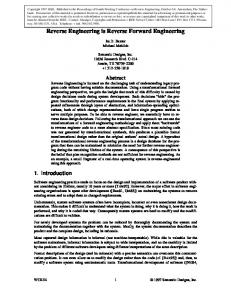
3. DESIGN We begin by giving a high-level overview of the algorithm. Figure 1 shows the sequence of processing stages performed by Tupni. A raw input is first segmented into basic fields (Section 3.3). The next processing stage identifies record sequences (Section 3.4). We then classify the records we have identified in the previous stage (Section 3.5). This gives us record types. We look for constraints at several processing stages. Our techniques for identifying constraints are described in Section 3.6. Most of the processing stages combine a baseline algorithm with an error correction scheme. The baseline algorithm captures the main idea underlying the processing stage. The error correction scheme accounts for the fact that real world applications do not always conform to the baseline algorithm. Most of the descriptions in this section show how Tupni analyzes a single run of a parsing application on a particular input. At the end of the section, we describe how Tupni aggregates the results of its analysis over several runs of the same application on different inputs. For a single run of the application, the sequence of instructions that is executed during this run is called the execution trace of the run. Each execution trace is associated with the list of binaries that were loaded during the run and the base addresses at which the binaries were loaded. This information is readily available from tools such as iDNA [4] that capture program execution traces. We refer to the byte positions in the input as offsets. We use the term position to identify instructions in the execution trace. For example, a particular mov instruction in the application binary may appear at multiple positions in the execution trace. We refer to sequences of contiguous positions in the execution trace as subsequences.

3.1

Background

Tupni assumes the availability of a taint tracking engine such as [10, 11, 31, 38]. These systems associate data structures with addresses in the application’s address space and update them as the application executes. In the simplest case, the data structures indicate whether the value stored at an address depends on input. When input data arrive in the application’s address space, the memory locations storing them are marked as tainted. Whenever an instruction reads and writes data, the data structure for the destination operand is updated depending on whether any of the source operands was tainted. More complex data structures allow more detailed information to be tracked, including which bytes in the input the value at a tainted memory location depends on or how that value was computed. We call the latter data structure a data flow graph [10].

Field Identification

Raw Input

Identification of Record Sequences

Sequence of Fields

Sequence of Records

Identification of Record Types

Sequence of Record Types

Figure 1: The processing stages of Tupni 0

1 2

2

34

56

1

78

16 17 18 19 20 21

13

...

5

Record 1

10

26

...

Record 2

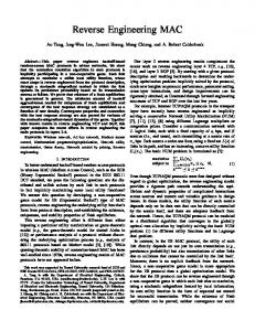
Figure 2: Running example input. 1 2 3 4

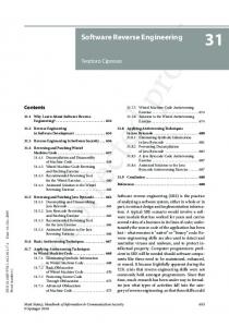
BYTE input[ BUF_SIZE ] ULONG num_records, i=0, offset=4 USHORT record_type, record_size FCT_PTR record_hdlr[NUM_REC_TYPES]

5 6

call read_input( input ) mov num_records, (ULONG *)&input[0]

7 loop: cmp 8 jeq

i, num_records end

9 10

mov mov

record_type, (USHORT *)&input[offset] record_size, (USHORT *)&input[offset+2]

11

call record_hdlr[record_type](&input[offset])

12 13 14 15 end:

add inc jmp

offset, record_size i loop

Figure 3: Example application.

3.2

Running Example

Throughout this section we will use a running example to help illustrate the stages of Tupni. For ease of exposition, we use a very simple synthetic input format and a similarly simple application that processes inputs from this format. The input format consists of a header followed by a sequence of records. The header has only one field. It specifies the number of records that follow. Each record starts with a two-byte field that specifies the record type, followed by a second two-byte field that specifies the size of the record in bytes. The remaining bytes of each record depend on the record type. This simple format is structurally similar to real world formats such as WMF, PNG, WMA and WMV. Figure 2 shows an example input from this format. The first field specifies the number of records as 2. The next 13 bytes make up the first record, and the following ten bytes make up the second record. These lengths are specified in the second field of each record. The first field of each record specifies its type (as types 1 and 5, respectively). Figure 3 shows a simple application that parses inputs from our example format. Our pseudo assembly notation can be mapped to working x86 machine code by assigning x86 registers to our variables and adding instructions to pass function call parameters. Line 5 reads the input into a sufficiently large buffer (input). Line 6 reads the first four bytes of input into num_records, which tells the application how many records it needs to process. Each iteration of the following loop (lines 7 to 14) processes one record. Lines 7 and 8 exit the loop after the last record has been

processed (i == num_records). Lines 9 and 10 read the type field and the length field of the record. Line 11 calls the handler function for the given record type. We assume that the function pointer array record_hdlr has been initialized with a handler function for each record type. These handler functions are part of the application, but not displayed in Figure 3 to keep the example manageable. Finally, line 12 sets offset to the beginning of the next record, and line 13 increments the index variable that counts how many records have been processed. The execution trace of running this program on the example input is 5,6,7,...,14,7,...,14,7, 8,15. That is, after executing lines 5 and 6, the trace contains two full iterations of the loop. Each segment 7,...,14 contains the instructions of the handler function between lines 11 and 12.

3.3

Field Identification

This first step partitions the input into short sequences of consecutive bytes that are likely to correspond to basic fields in the input format. Typically, several consecutive input bytes will be mapped to a larger field such as a 32-bit integer. We deduce this mapping by observing the operands of CPU instructions. Given an operand of a CPU instruction in the execution trace, we call the longest sequence of tainted bytes from contiguous offsets contained in the operand a chunk. Our algorithm identifies all chunks in the execution trace by stepping through the trace and inspecting the operands of each instruction for taint. We ignore move instructions as they do not process the operand and contain little information about field sizes. Any byte of the input that is read by the application will be contained in at least one chunk. In general, a chunk may be accessed by multiple instructions. We keep track of this by assigning a weight w(c) to each chunk c. The weight of a chunk is simply the number of instructions in the execution trace that access the chunk (ignoring move instructions). In this way, by observing the operands of x86 instructions, we can identify chunks contained in 8-, 16-, 32- and 64-bit integer operands as well as floating point chunks. We can also recognize big-endian integers if we see a chunk with reversed bytes. Currently we track input chunks at byte granularity; we believe it takes only engineering efforts to refine this to bit granularity.

Running Example. The first time the application reaches line 7, the second operand of the cmp instruction is tainted with the first four bytes of the input. This causes Tupni to create a chunk [0, 3] for offsets 0 to 3 and to assign it weight 1. Note that the mov instruction in line 6 does not create a chunk. It simply propagates taint into num_records. Analogous statements apply to lines 9 and 10. The next chunk [4, 5] is created in line 11 because record_type is tainted with offsets 4 and 5. The instructions executed by the record handler function called in line 11 will typically create further chunks for the offsets inside the record. Since our simple example does not specify handler functions, we ignore this part of the execution trace. Line 12 creates the chunk [6, 7] since record_size is tainted with offsets 6 and 7.

In the second loop iteration, line 7 increases the weight of [0, 3] to 2, and lines 11 and 12 act as in the previous iteration, creating chunks [17, 18] and [19, 20], respectively. Finally, the third execution of line 7 raises the weight of [0, 3] to 3. The final set of chunks is [0, 3], [4, 5], [6, 7], [17, 18] and [19, 20]; plus any chunks generated by the handler functions.

3.3.1

Error Correction

The next step is to map chunks to fields. A general difficulty is that, during the course of its execution, an application may access the same offset using different operand types. Thus, an offset may be contained in different chunks. The most common application behavior that gives rise to such inconsistencies includes (a) bulk accesses (memory copies, checksums, etc.) in which the application reads a part of the input without concern for field boundaries and (b) optimized string processing code that uses 32-bit (or larger) operations to process an ASCII or unicode string. The goal is to find a consistent subset S of chunks such that we can identify each chunk in S with a field. Tupni has to find a subset S of chunks such that all chunks in S are disjoint and the combined weight of the chunks in S is maximized. This is an instance of the weighted Maximum k-Set Packing problem. While it is intractable to even approximate the optimal solution under worst-case analysis [21], the problem instances we obtain from real-world execution traces are quite simple with little overlap among chunks. We use the greedy algorithm [7] to compute S and identify the chunks in S with input fields. Based on our evaluation (Section 4), this simple algorithm seems sufficient. In general, the fields we have found may not cover the entire input. In many cases, the application never accesses certain parts of the input. Thus, observing the application reveals no information about these parts. All Tupni can do is to mark the contiguous gaps between fields as virtual fields. In our simple example, all chunks are disjoint. Thus, Tupni promotes all chunks into fields. Again, ignoring the handler functions, offsets [8, 16] and [21, 26] are gaps between fields. Tupni adds [8, 16], [21, 26] as virtual fields.

3.3.2

Strings

We consider strings as regular record sequences. Thus, we have no string fields. Given a string, Tupni will recognize the string characters as fields. The next section will describe how Tupni infers that these character fields form a string as part of the more general framework for recognizing record sequences. A special problem arises for strings because many applications use optimized string processing code that uses 32-bit rather than 8bit or 16-bit instructions to access strings. This could cause string characters to be misclassified as 32-bit integers. Fortunately, the optimized string processing code is easy to recognize. All instances we have observed on Windows and Linux involve boolean and comparison operations with two or three specific constants. If we recognize optimized string processing code, we ignore the corresponding instructions in the calculation of chunk weights.

3.4

Identification of Record Sequences

This section describes how we identify record sequences. As defined in Section 2.2, a record sequence covers a contiguous sequence of offsets in the input. Our algorithm is based on the observation that applications have to use a loop or recursive calls to process an unbounded sequence of records. We have developed Tupni for the common case of loops. We believe that similar techniques can be used to handle recursive calls. The algorithm proceeds in the following three steps: (a) Identify

all loops that are executed in the execution trace; (b) For each loop, find the relevant input fields that are accessed in each loop iteration; (c) For each loop that processes relevant input fields, identify the record boundaries. The rest of the section describes each of the three steps in detail.

3.4.1

Loop Identification

The first problem is to find loops in the application. The solution is to search for cycles in the control flow graph (e.g., [3]). This method yields a complete list of loops and their relationship. We only consider loops with a single entry point. The next task is to map the loop information to the execution trace. Given a loop (a cycle in the control flow graph), we can map each instruction in that cycle to the program counter (EIP) value at which the instruction was stored when the execution trace was created. This makes use of the information about loaded binaries mentioned in Section 3.1. For each loop, we maintain a compact representation of the set of EIP values of the instructions in the loop. We also store the EIP of the unique entry point of each loop. Tupni tests for each position in the trace and for each loop whether the EIP value at that position is contained in the set of EIP values of the loop. The result of this process is the list of all subsequences of the execution trace that correspond to the execution of a loop (labeled with an identifier for that loop). Finally, we identify the individual loop iterations within each subsequence. We mark the beginning of an iteration at the points where the execution trace hits the (unique) entry point of the loop.

Running Example. The code in Figure 3 has a single loop (cycle in the control flow graph) in lines 7 to 14. Line 7 is the only entry point of this loop. Let A be a label for this loop. There may be further loops in the handler functions. Those would be recognized as nested within loop A. Since the execution trace in Section 3.2 uses line numbers rather than EIP values, there is no mapping to be done. Otherwise, we would have to look up at what base address the application binary was loaded when the execution trace was created. Comparing the line numbers in the execution trace in Section 3.2 with the line numbers of our loop (7 to 14), we find that the subsequence that starts at the third instruction in the trace and ends right before the last instruction corresponds to the execution of loop A. Tupni identifies iterations by looking for the entry point of loop A (line 7) within the subsequence. It finds three occurrences of line 7 in the subsequence (at the very beginning, toward the middle and at the end. Thus, Tupni splits the subsequence into three iterations at these three positions. The third iteration contains only lines 7 and 8.

3.4.2

Identifying Relevant Fields

In the following, we will also use the term loop as a shorthand for “a subsequence of the execution trace labeled by a loop identifier”. Most loops executed by applications do not process record sequences from the input. We are only interested in those loops that iterate over multiple input fields. In this step, we identify such loops. Consider a loop l and let n be the number of iterations that were executed. We define sets Ii (1 ≤ i ≤ n) as follows: An instruction (identified by its instruction pointer (EIP) value) is contained in Ii if the instruction accesses a field during the i-th loop iteration that it does not access in any other iteration of l. If In is empty then we treat the loop as if it had only n − 1 iterations. This special case is necessary since the last iteration of a loop is often not a true iteration, but only a check of the termination

FindRecordBoundaries( 1. IN n, // number of loop iterations 2. IN (I1 , . . . , In ), // iteration dependent instructions for each loop iteration 3. OUT (s1 , . . . , sn ),// start offset of each record 4. OUT (e1 , . . . , en ) )// end offset of each record 5. 6. for ( j from 1 to n ) sj = −1; // mark start of record j as unknown 7. 8. for ( j from 1 to n ) { 9. if ( sj == −1 ) 10. then sj = min{ Offset( Field( inst ) ) : inst ∈ Ij } 11. I = { inst∈ Ij : Offset( Field( inst ) ) = sj } 12. for ( i from j + 1 to n ) 13. if ( I ∩ Ii 6= {} ) 14. si = min{ Offset( Field( inst ) ) : inst ∈ Ii ∩ I} 15. } 16. 17. for ( j from 1 to n − 1 ) ej = sj+1 − 1; 18. en = max{ Offset( Field( inst ) ) + sizeof( Field( inst ) ) : inst ∈ In }

Figure 4: Identification of record boundaries condition (as in our example, where the third iterations consists only of lines S 7 and 8). We call i Ii the set of iteration dependent instructions. We call a loop iteration dependent if Ii 6= {} for all i ∈ {1, . . . , n − 1}. We compute the sets Ii for all loops identified in the previous step. At the end of this analysis, we obtain the list of iteration dependent loops in the execution trace and, for each iteration dependent loop, the sets Ii of its iteration dependent instructions.

Running Example. I1 = {9, 10, 11} and I2 = {9, 10, 11}. Thus, the loop is iteration dependent. For example, line 9 accesses field [4, 5] in the first iteration and only in the first iteration. Thus, it belongs to I1 , It also accesses field [17, 18] in the second iteration and in no other iteration. Thus, it also belongs to I2 . On the other hand, line 7 is not iteration dependent. It accesses the same field ([0, 3]) in all iterations.

3.4.3

Identifying Record Boundaries

In this step, we group fields into records and identify the record boundaries. We make use of the fact that, given the definitions of Section 2.2, a record is a contiguous sequence of fields and a record sequence consists of contiguous records. Furthermore, we assume that the loop processes records in the order in which they appear in the input. Loops that do not satisfy this assumption are ignored. However, we can handle loops whose iterations access fields in records outside the record currently being processed. Our algorithm is shown in Figure 4. Tupni calls this algorithm for every iteration dependent loop. For ease of presentation, the figure assumes that each iteration dependent instruction inst accesses only one field (Field(inst)). This assumption has no fundamental importance. Its only purpose is to remove tedious details from Figure 4. For any field f, let Offset(f) denote the offset in the input of the first byte of f. The algorithm sets the start of the first record to min{ Offset(f )}, where the minimum is taken over all fields that are accessed by iteration dependent instructions in the first iteration of the loop (line 10). Next, in line 11, it identifies the set I of iteration dependent instructions that access the field at the beginning of the first record in the first iteration. The scheme now uses the heuristic that the instructions in I are likely to access the beginning of a record whenever they appear. Thus, it looks for instructions from I in each iteration (line 13) and sets the start of the corresponding record accordingly (line 14). The process is re-

peated (line 8) for the case that an iteration does not use any instruction from I. Finally, the end of each record is set to the offset immediately before the start of the next record (line 17). The end of the last record is set to the last input byte accessed by any iteration dependent instruction in the last iteration (line 18). This procedure is performed for all iteration dependent loops. A loop is ignored if the computed record start addresses are not increasing.

Running Example. The algorithm sets s1 = 4 (line 10), since I1 = {9, 10, 11}, Field(9) = [4, 5] and Offset([4, 5]) = 4. That is, 4 is the smallest offset accessed by instructions in I1 . Line 11 sets I = {9, 11} since both instructions accessed field [4, 5] in the first iteration. Next, it sets s2 = 17 since instructions 9 and 11 access field [17, 18] in the second iteration. Line 17 sets e1 = s2 − 1 = 16. Finally, line 18 sets e2 = 20 the largest offset accessed by an instruction from I2 . While all other values are correct, e2 is somewhat too small. This is primarily the result of the fact that we have ignored the handler functions called in line 11 of the example application.

3.4.4

Length Determination

We also output for each record sequence how its length is determined. We consider the following three cases: (a) The length is determined by a termination record (e.g., null terminated ASCII strings); (b) The length is determined by a separate length field; (c) The length is fixed and implicitly determined by the protocol specification. Tupni identifies case (a) (termination record) by checking all equality comparisons between a constant and the value of a field accessed by an iteration dependent instruction. We classify the record sequence as case (a) if we observe a constant for which there is such an equality check that evaluates to false in each iteration (up to but not including the last iteration) and if the last iteration contains an equality check with the same constant that succeeds. For case (b) (length fields), we use a technique from Polyglot [6]: We identify fields that are accessed to compute the termination condition of loops. If we do not recognize case (a) or (b), we classify the record sequence as case (c) (implicit length).

3.5

Record Type Identification

Typical formats specify record sequences such that records come from a small set of classes (the record types of Section 2.2). So far, we have identified record sequences, found out how the length of the record sequence is determined and found the boundaries of the individual records in a sequence. In this step, Tupni tries to find the record type for each record. More precisely, Tupni considers two records as belonging to the same record type if the loop iterations that process the records execute “mostly” the same instructions. This is based on the observation that applications typically have a separate handler function for each record type. The problem is complicated by the fact that record sequences may be nested. That is, there are sequences whose records contain other sequences. If a record contains a child record sequence then the instructions that process it may depend heavily on the particular instance of the child record sequence it contains. Thus simply looking for similar instruction sequences will not solve the problem. Let l be an iteration dependent loop, and let r be the record sequence l processes. Let n be the number of records in r. For i ∈ {1, . . . , n}, we define Qi to be the subset of instructions from Ii that access fields in the i-th record of r. We compute the sets Qi for every record sequence we have identified in the previous step. The set Qi is a superset of the set of instructions that we consider

relevant. As outlined above, if records in r contain nested record sequences then records of the same record type may have widely different sets Qi . Therefore the next step of our algorithm is to transform each set Qi into a set Q0i as follows. Tupni collapses every segment of the instruction trace that contains an execution of a child loop into a single virtual instruction. This instruction is assigned a virtual identifier (virtual EIP) such that two virtual instructions have the same identifier if and only if they correspond to executions of the same loop. Q0i is set to Qi , except that all instructions in the child loop execution are removed from the Qi and replaced by the identifier of the virtual instruction that represents the child loop. The net effect of this transformation is that iteration dependent loops that process child record sequences contribute a single virtual instruction to the Q0i of the parent record. This way, it only matters whether the child loop was executed, but not what happened during its execution. In summary, Tupni considers each record sequence r that was identified in the previous step and computes Q0i for every record i in r. Tupni classifies two records i, j as having the same type if Q0i = Q0j .

Running Example. Recall that, in the previous step, Tupni had identified one record sequence with two records. We have Q1 = {9, 10, 11} ∪ h1 and Q2 = {9, 10, 11} ∪ h5 , where h1 and h5 denote the instructions in record_hdlr[1] and record_hdlr[5], respectively, that access the record sequence. Typically, h1 and h5 will be different. If neither of the two records contains a nested record sequence then Q01 = Q1 and Q02 = Q2 . In order to examine the other case, let record_hdlr[1] contain a loop that iterates byte-bybyte over the payload of record 1 (offsets 8 to 16). In this case, h1 contains up to 9 different instructions (for the nine loop iterations from offset 8 to offset 16). Q01 would now be Q01 = {9, 10, 11, v1 }, where v1 is a unique identifier for the loop in record_hdlr[1].

3.6

Constraint Identification

This section describes how Tupni identifies conditions on the values of fields that an input must satisfy to be valid. This includes relations between the values of multiple fields. We call such conditions constraints. Tupni considers three types of constraints.

Symbolic Predicates. The dynamic data flow analysis engine [10] used by Tupni outputs a sequence of conditions on the input (symbolic predicates) that were checked by the application during its execution. These conditions encode the application’s execution path. In general, some of these conditions will represent properties that any valid input must have while other conditions simply represent properties of the particular input the application was run on. For the purpose of gathering constraints on the format, we are interested in the former, but not in the latter. Tupni generates constraints on the value of single fields (singlevalue constraints) as follows. For each input field i, Tupni outputs the conjunction of all symbolic predicates of the form f (input[i]){< , =, >, 6=}y, where f is a function that depends on nothing but input values and constants that are hard coded into the application (e.g., immediate operands of x86 instructions). In addition, we ignore all symbolic predicates associated with checks for termination values of record sequences, as the information contained in them is already accounted for by the analysis of length determination (Section 3.4). Tupni also outputs symbolic predicates of the form input[x] =

f (input[y], input[z], . . .), where f is a function that depends on nothing but input values and constants that are hard coded into the application. This type of constraint can capture many types of checksum calculations. We call such constraints functional constraints. The constraints generated by this simple procedure may be particular to the input the application was run on and may not represent the input format in general. This is a general limitation of dynamic analysis. Recent systems such as Bouncer [9] and ShieldGen [14] were designed to overcome this limitation in a different application domain. We believe that the techniques employed by these systems could be used to eliminate most of the remaining input specific conditions.

Inter-Message Dependencies. An inter-message constraint for a multi-message network protocol determines the value of a field in a later message based on the values of one or more fields in an earlier message. Typical examples include session IDs and sequence numbers. Tupni inspects all attempts by the application to send data to the network. If it finds tainted data in an outgoing message, it outputs the associated data flow graph that describes how the tainted output field depends on the previous input.

Length Fields. Tupni uses three techniques for identifying length fields. The first technique makes use of the semantics of certain platform functions as described in Section 3.7. The other two techniques are similar to techniques used in Polyglot: identifying fields used to compute pointers that are used to access other input fields and identifying fields that are accessed to compute the termination condition of loops that process record sequences.

3.7

Platform-Specific Functions

Knowledge of the semantics of platform specific functions such as system calls, application programming interface (API) functions and functions in runtime libraries can significantly enhance the accuracy and functionality of Tupni. The idea of using the semantics of library calls has been used in Bouncer [9]. However, the way in which Tupni makes use of function calls is quite different from the method in Bouncer. As a preliminary step, we have added specifications of six string processing functions and 20 memory allocation functions to Tupni. These specifications are used in the following areas: • Field identification: Use of an input chunk as a function parameter can provide strong evidence that the chunk is a field. This evidence is incorporated into the field recognition step by increasing the weight w(c) of the chunk if Tupni sees a call to a known function in the execution trace. More extensive use of function semantics has the potential of providing very detailed information about the types and semantics of input fields. We leave this for future work. • Identification of record sequences: Functions may have record sequences (or pointers to them) as parameters. For example, a call to a standard string processing function with a charpointer that points to tainted data provides strong evidence that the pointer marks the start of a string. • Constraint identification: function calls may provide information about different kinds of constraints. We have used knowledge of memory allocation functions to identify length fields. For example, a call to malloc with a tainted size

parameter provides evidence that this parameter is a length field. In general, we do not consider the parts of the execution trace that are spent inside any of the known functions in our analysis. Effectively, this collapses calls to these functions into a single virtual instruction with special semantics.

3.8

Output Format Input ::= F1 :D S1[F1] S1

::= R1 | R2 | ...

R1

::= F2 :W F3 :W { F3 = SIZE(R1) } ...

R2

::= F4 :W F5 :W { F5 = SIZE(R2) } ...

Figure 5: The output format for the running example. At this point, Tupni’s analysis of a single input is complete. Tupni outputs the fields and record sequences it identifies in an enhanced BNF format. An example of this output format is shown in Figure 3.8 for the running example. Tupni generates a rule that lists the top-level fields and record sequences in the order of their positions in the input. We refer to this rule as the root rule. For each record sequence, Tupni generates an alternation rule to cover all its record types. For each record type Tupni generates a rule to list its fields and child record sequences. This process continues recursively for all record sequences and record types. In addition, Tupni outputs constraints in the enhanced BNF format.

3.9

Aggregation over Multiple Inputs

So far, we have discussed how Tupni analyzes a single execution trace – corresponding to a single input. If multiple inputs of the unknown format are available, the application can be run on each of them, and Tupni can perform its analysis on each of the resulting execution traces. The last step is to combine the individual results into a single format specification. To do so, Tupni matches fields, record sequences, and record types across different execution traces. Consider two execution traces from the same application, but different inputs. Tupni considers two base fields from two execution traces to match if they are accessed by the same set of instructions. Tupni considers two record sequences from two execution traces to match if they are processed by the same loops (identified by the unique loop entry point). Finally, Tupni considers two records from matching record sequences to have the same type if their respective sets Q0i are equal. After identifying all matching fields, record sequences and record types in the two execution traces, Tupni merges the BNF rules for each of the execution traces into a single set of BNF rules. Tupni first identifies the pairs of BNF rules that can be merged. These include the root rules and the BNF rules of matched record sequences and record types. To merge BNF rules of matched record sequences, Tupni simply creates a new alternation rule that includes all record types in the old rules. Tupni merges the root rules and rules of matched record types in two steps. It first aligns the list of fields and record sequences using the type-based sequence alignment technique proposed in [12]. If all fields and record sequences

are perfectly matched, it means that the two rules are identical; Tupni simply keeps one. Otherwise, it creates a new alternation rule for each pair of unmatched fields or record sequences. Then it creates a new rule that lists matched fields and record sequences as well as the alternation rules for unmatched fields or record sequences.

4.

IMPLEMENTATION AND EVALUATION

We have developed a prototype of Tupni. Our dynamic data flow engine was built on a re-implementation of the Vigilante system [10]. Our prototype system uses iDNA [4], a binary program translator, to capture and replay program execution traces. Our system works on x86 instructions directly. Excluding the code of the original Vigilante and iDNA, our Tupni prototype has 14,000 lines of C++ and 4,100 lines of Perl. In this section, we first describe our experimental setup and evaluation methodology. After that, we present our experimental results.

4.1

Experimental Setup

Our evaluation is divided into two parts. We first tested how accurately Tupni can reverse engineer the format of a single input message or file. Then we evaluated its capability of generalizing the input format over multiple inputs. In the first set of experiments, we evaluated Tupni on both files and network messages. We tested five binary files (WMF, BMP, JPG, PNG and TIF), three binary network messages (DNS response, TFTP data and RPC bind request), and two text network messages (HTTP GET request and FTP port command). We selected these input formats because they are representative protocols and were studied in previous work. We intentionally avoided types of input formats for which we knew a priori that our prototype would perform poorly (see Section 7 for a discussion of these formats). For instance, our prototype does not work well if the field boundaries of a format do not coincide with byte boundaries due to its bytebased taint tracking. For the compressed image files among our test cases, we used Tupni to reverse engineer the container file format and ignored the format of the compressed data blobs. We used WMF, the DNS response message, and the HTTP request message to guide our design. We ran the remaining seven test cases without changing the prototype. For each input, we recorded an execution trace of a binary program parsing and processing it on Windows XP Professional SP2. Then we fed the execution trace to Tupni to reverse engineer the format. The inputs and binary programs are listed in Table 1. In all our test cases, Tupni can reverse engineer the formats in at most 5 minutes on a 3GHz machine running Windows XP Professional SP2.

4.2

Evaluation Methodology

In our first set of experiments on single test inputs, we focused our evaluation on accuracy, that is, how accurately Tupni can identify the fields, record sequences, record types, and constraints in the test inputs. Tupni automatically outputs the reverse engineered formats in an enhanced BNF format (referred to as the Tupni format). In order to evaluate the accuracy of Tupni’s output, we compare the format specification Tupni produced for each test case with the published specification [1, 2, 16, 20, 28, 34, 37, 39, 40] (referred to as the published format) for the same format and identify discrepancies. In our second set of experiments, we focus our evaluation on completeness, that is, how well Tupni can infer a more complete input format over multiple inputs. It is hard to compare our results with previous work [6, 12, 26,

Format Name WMF BMP JPG PNG TIF DNS response RPC bind TFTP data HTTP request FTP port

Application gdi32.dll mspaint.exe gdiplus.dll gdi32.dll gdiplus.dll nslookup.exe rpcss.dll tftp.exe inetinfo.exe ftpsvc2.dll

Execution Trace (instructions) 3.2M 12.0M 15.7M 12.2M 12.0M 4.7M 128K 5.5M 156M 121M

Input Size (B) 4594 3126 3224 3543 4337 46 164 28 107 28

Run Time (min) 5 1 3 3 3