Two Behavioural Lambda Models - Dipartimento di Informatica - UniTo
Recommend Documents
Oct 25, 2008 - unreachable due to client mobility; and feedback ratings col- lected during random ...... 2http://code.google.com/android/ peer-to-peer system,â ...
inspires our definition of relevant type inference systems when intersection -as ... Following the standard definition of relevance logic, see [9], a system is ...
Jun 19, 2008 - X-Hinter, we describe a Java API that provides a set of li- braries and tools to build social ... formation (e.g., eBlogger, MySpace, Facebook). People can ... uj is defined as the. 1http://wiki.limewire.org/index.php?title=Overview.
Jun 14, 2013 - A modificatory provision is a change made to one or more .... sion of a normative provision does not affect its force. ...... IOS Press, 2002.
KEN, the outcome of the action is necessarily failed. Other formulas can be ...... 2004, pp. 535â541. [21] J. Whaley, Javabdd package â project summary page at.
Jun 19, 2008 - the Limewire P2P file sharing application. This application works on top of the Gnutella network, so all the information about the network, such ...
Jun 14, 2013 - XML format. In particular, we refer throughout the paper to a a standard format for Italian Legal Text, the NormeIn-. Rete (NIR) format.1. The NIR ...
of sequences of interleaved actions, providing a normal form for types assigned to processes. In the filter model obtained via the introduced type system, any ...
ABSTRACT. This paper presents a method for the numerical analysis of charge-pump Phase-Locked Loops in time domain, using behavioural modelling of ...
Luca Paolini1 ,2. Dipartimento di Informatica. Universit`a di Torino (ITALIA). Elaine Pimentel1 ,2. Departamento de Matemática. Universidade Federal de Minas ...
Luca Paolini1. Dipartimento di Informatica. Universit`a di Torino. Torino, Italy. Mauro Piccolo2. Dipartimento di Informatica. Universit`a di Torino. Torino, Italy.
that the system need to account for are (1) the diet that the user intends to follow, (2) the food ... Automatic reasoning and Natural Language Generation (NLG).
of bound names is intended to avoid capturing the free name x. We use. âââââ. [a = b] to denote a sequence of matchings [a1 = b1] ··· [am = bm] (m > 0),. ââ νc.
authors in studying security and privacy issues of web data. The proposed approach is ... In case we are given a target security policy for a distributed system .... representation of XML documents) store is accessible to the process with role ...
paper P1 in which one of its authors says that he has published a paper with him ... case of distributed policies and delegation, e.g., âadministrator says that Alice.
tralized and encrypted P2P architecture providing plausible anonymity for its par- ..... contract with the technology provider (e.g., Akamai for CDN infrastructures).
25 ott 2012 ... Lucio Russo, fisico teorico, Professore di Metodi Matematici a Roma, ... Russo si
pone l'obiettivo di 'controllare' se le caratteristiche ...
May 31, 2009 - Î-normal forms are not input values. Luca Paolini: Call-By-Value Lambda Calculus. Paris, May 2009 â5/31. Confluence. Theorem 2. M ââ.
As proved in [HL99], we can give a finitary logical description of HLâ us- ing intersection types. In other words we can define an intersection type theory. HLâ.
[[(λx.x)y]]Dâ¤ Ï ... [[y]]Dâ¤ Ï . As well known, whenever FD ⦠GD = Id[DâD], the λ-structure ãD ...... The Y-combinator in Scott's λ-calculus models (revised version).
tration of both physical and virtualized clusters with no single point of failure. ... Cluster Manager enables the system administrator to create, save, restore Xen-based virtual ... on a novel disk abstraction layer, which enables the fast, space-ef
Horstmann-Concetti di informatica e fondamenti di Java 2. 1. Capitolo 17
Introduzione alle strutture di dati. Capitolo 17. Introduzione alle strutture di dati ...
A well-known example is the Java programming language. ... Some of the above mentioned calculi deal also with the key issue of security, namely ..... Page 11 ...
Dec 17, 2001 - This technique relies on the use of a software program (simulator) in order to ... makes it very problematic to build a full-featured simulator. For.
Two Behavioural Lambda Models - Dipartimento di Informatica - UniTo
Corrado BÙhm and Mariangiola Dezani-Ciancaglini. λ-terms as total or partial functions ... Mariangiola Dezani-Ciancaglini and Silvia Ghilezan. ... William W. Tait.
Two Behavioural Lambda Models Mariangiola Dezani-Ciancaglini1? and Silvia Ghilezan2?? 1
Dipartimento di Informatica, Universit`a di Torino, Torino, Italy [email protected] 2
Faculty of Engineering, University of Novi Sad, Yugoslavia [email protected]
Extended abstract Abstract. We build two inverse limit lambda models which characterize completely sets of terms having similar computational behaviour. More precisely for each one of these sets of terms there is a corresponding element in at least one of the two models such that a term belongs to the set if and only if its interpretation (in a suitable environment) is greater than or equal to that element. This is proved by using the finitary logical description of the models obtained by defining suitable intersection type assignment systems.
1
Introduction
The aim of this paper is to present two lambda models which completely characterize well-known computational properties of lambda terms. We consider nine computational properties of lambda terms and corresponding nine sets of lambda terms: the set of normalizing, head normalizing, weak head normalizing lambda terms, those corresponding to the persistent versions of these notions, and the sets of closable, closable normalizing and closable head normalizing lambda terms. We build two inverse lambda models D∞ and E∞ , according to Scott [24], which completely characterize each of the mentioned sets of terms. More precisely for each one of the above nine sets of terms there is a corresponding element in at least one of these models such that a term belongs to the set if and only if its interpretation (in a suitable environment) is greater than or equal to that element. This is proved by using the finitary logical descriptions of the models D∞ and E∞ obtained by defining two intersection type assignment systems in the following way. First, we construct the sets TD and TE of types which are generated from atomic types corresponding to the elements of D0 and E0 , by the function type constructor and the intersection type constructor. Then ?
??
Partially supported by EU within the FET - Global Computing initiative, project DART ST2001-33477 , and by MURST Cofin’01 project COMETA. The funding bodies are not responsible for any use that might be made of the results presented here. Partially supported by grant 1630 “Representation of proofs with applications, classification of structures and infinite combinatorics” (of the Ministry of Science, Technology, and Development of Serbia).
we define the sets FD and FE of filters respectively on the sets TD and TE . Following Scott [26], Coppo et al. [8], and Alessi [3], we will show that the sets FD (ordered by subset inclusion) and FE and the corresponding inverse models D∞ and E∞ are isomorphic as ω-algebraic cpos. This isomorphism falls in the general framework of Stone dualities (Johnstone [14]). This framework later received a categorically principled explanation by Abramsky in the broader perspective of “domain theory in logical form” [1]. The interest of the above isomorphism lies in the fact that the interpretations of lambda terms in D∞ and E∞ are isomorphic to the filters of types one can derive in the corresponding type assignment systems (Alessi [3]). This gives the desired finitary logical descriptions of the models. Therefore an equivalent of the primary complete characterization can be stated: a term belongs to one of the nine sets mentioned if and only if it has a certain type (in a suitable context) in one of the obtained type assignment systems. In order to prove one part of this property we apply the so called reducibility method. This method is a generally accepted way for proving the strong normalization property of various type systems (Tait [28], Tait [29], Girard [13], Krivine [16], [17], Mitchell [20]). The reducibility method is also used in Leivant [18] and Gallier [11] for characterizing strongly normalizing terms, normalizing terms, head normalizing terms, and weak head normalizing terms by their typeability in various intersection type systems. In Dezani et al. [10] the reducibility method is applied to characterizing both the mentioned sets of terms and their persistent versions. In all these papers different properties are characterized by means of different type assignment systems: so the novelty of the present approach is that we characterize all nine computational properties of terms by means of only two type assignment systems, which induce λ-models. Moreover in all the papers mentioned different computational properties require different type interpretations in the reducibility method, whereas we adapt the reducibility method using only two type interpretations for all nine computational properties. In the other direction of the proof the most intriguing part is the one concerning the persistently normalizing terms, which requires the characterization of these terms presented in Dezani et al. [10]. Lastly we remark that there are essentially two semantics for intersection types in the literature and that the present paper deals with both of them. The set-theoretical semantics, originally introduced in Barendregt et al. [5], generalizes the one given by Scott for simple types (Scott [25]). The meanings of types are subsets of the domain of discourse, arrow types are defined as logical predicates and intersection is the settheoretic intersection. This semantics is at the basis of our application of the reducibility method. The second semantics views types as compact elements of Plotkin’s λstructures (Plotkin [22]). According to this interpretation, the universal type denotes the least element, intersections denote joins of compact elements, and arrow types allow to internalize the space of continuous endomorphisms. This semantics allows us to obtain the isomorphisms between the models D∞ , E∞ and the sets FD , FE of filters of types. The paper is organized as follows. In Section 2 the models D∞ and E∞ are built. The corresponding intersection type assignment systems are defined in Section 3. The main result is a complete characterization of computational behaviours of terms by their
typeability in the corresponding type systems. This is stated in Section 4. For lack of space some proofs are omitted. A preliminary version of the present paper (dealing only with the first six sets of terms) was presented at the International Workshop on Rewriting in Proof and Computation (RPC’01, Tohoku University 25-27/10/2001, Sendai, Japan) [9] and at the Types Workshop (TYPES 2002 24-28/04/2002, Nijmegen, The Netherlands).
2
The Models
We use standard notations for lambda terms and beta reductions. Definition 1 (The set Λ of lambda terms). The set Λ of (type-free) lambda terms is defined by the following abstract syntax. Λ ::= var | (ΛΛ) | (λvarΛ) var ::= x | var0 We use x, y, z, . . . , x1 , . . . for arbitrary term variables and M, N, P, . . . , M1 , . . . for arbitrary terms. In writing terms we assume the standard conventions on parentheses and dots [6]. FV(M ) denotes the set of free variables of a term M . By M [x := N ] we denote the term obtained by substituting the term N for all the free occurrences of the variable x in M , taking into account that free variables of N remain free in the term obtained. The axiom of β-reduction is (λx.M )N →β M [x := N ]. A term of the form (λx.M )N is called a β-redex. The transitive reflexive closure of →β is denoted by → →β . A term is a normal form if it does not contain β-redexes. We introduce now the computational behaviours of lambda terms we want to characterize. Definition 2 (Normalization properties). i) A term M has a normal form, M ∈ N , if M reduces to a normal form. ii) A term M has a head normal form, M ∈ HN , if M reduces to a term of the form → → → λ x .y M (where possibly y appears in x ). iii) A term M has a weak head normal form, M ∈ WN , if M reduces to an abstraction or to a term starting with a free variable. For each of the above properties, we also consider the corresponding persistent version (see Definition 3). Persistently normalizing terms have been introduced in B¨ohm and Dezani [7]. Definition 3 (Persistent normalization properties). →
→
i) A term M is persistently normalizing, M ∈ PN , if M N ∈ N for all terms N in N . → ii) A term M is persistently head normalizing, M ∈ PHN , if M N ∈ HN for all → terms N . → iii) A term M is persistently weak head normalizing, M ∈ PWN , if M N ∈ WN for → all terms N .
We also consider the reducibility of terms to closed terms, to closed normal forms, and to closed head normal forms. Definition 4 (Closability properties). i) A term M is closable, M ∈ C, if M reduces to a closed term. ii) A term M is closable normalizing, M ∈ CN , if M reduces to a closed normal form. iii) A term M is closable head normalizing, M ∈ CHN , if M reduces to a closed head normal form. Example 1. Let I ≡ λx.x, ∆ ≡ λx.xx, Y ≡ λf.(λx.f (xx))(λx.f (xx)), K ≡ λxy.x. – λx.x∆∆ ∈ N , but λx.x∆∆ ∈ / PWN (hence λx.x∆∆ ∈ / PHN ), since (λx.x∆∆)I → →β ∆∆ ∈ / WN . Notice that λx.x∆∆ ∈ / PN since I ∈ N . Lastly λx.x∆∆ ∈ CN . – λx.y(∆∆) ∈ PHN , but λx.y(∆∆) ∈ / N. – λx.x(∆∆) ∈ HN , but λx.x(∆∆) ∈ / N and λx.x(∆∆) ∈ / PWN , since (λx.x(∆∆))∆ →β ∆(∆∆) ∈ / WN . Moreover λx.x(∆∆) ∈ CHN , but λx.x(∆∆) ∈ / CN . – YK ∈ PWN , but YK ∈ / HN , hence YK ∈ / PHN . – λx.∆∆ ∈ WN , but λx.∆∆ ∈ / HN and λx.∆∆ ∈ / PWN , since (λx.∆∆)M → →β ∆∆ ∈ / WN . Moreover λx.∆∆ ∈ C, but λx.∆∆ ∈ / CHN , hence λx.∆∆ ∈ / CN .
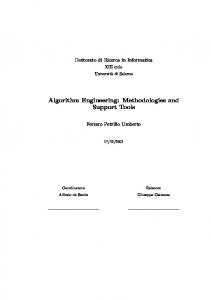
The following proposition, represented pictorially by Figure 1, sums up the mutual implications between the above notions:
Proposition 1. The following strict inclusions hold: PN PN PHN CN CN CHN
N PHN HN CHN N HN .
HN PWN
WN WN
C
Λ
Λ
No other inclusion holds between the above sets. Moreover PHN = PWN ∩ HN CHN = C ∩ HN C ∩ PHN = ∅
PN PHN ∩ N CN = C ∩ N C ∩ PN = ∅.
Proof. A persistently weak head normalizing term M is either an unsolvable term of order ∞ (as defined in Abramsky and Ong [2]), i.e. for all n there is N such that M =β λx1 . . . xn .N , or it is a solvable term such that the head variable of its head normal form is free. In fact if M is an unsolvable term of a finite order, i.e. M =β λx1 . . . xn .N → where N is unsolvable and it does not reduce to an abstraction, then M N ∈ / WN where → → → → → → → N are n arbitrary λ-terms. If M =β λ x y z .y N we get M X(∆∆) Z → →β ∆∆N 0 ∈ / → → → → WN , where X has the same length as x , Z has the same length of z , ∆ is defined in → → → → → → Example 1, and N 0 = N [ x := X, y := ∆∆, z := Z ]. The above discussion also shows that a persistently head normalizing term is a solvable term such that the head variable of its head normal form is free. So we get: PHN = PWN ∩ HN . From the same example we have that a necessary condition for a normalizing term to be a persistently normalizing term is that the head variable of its normal form is free. This condition is not sufficient, since for example (λx.y(xx))∆ →β y(∆∆). Being λx.y(xx) ∈ PHN and λx.y(xx) ∈ N this term shows that: PN
PHN ∩ N .
For closable terms we clearly have: CHN = C ∩ HN C ∩ PHN = ∅
CN = C ∩ N C ∩ PN = ∅.
The above discussion gives some inclusions between the current sets of terms, and Example 1 shows differences between them. The remaining inclusions easily follow by definition. Our goal is to build two inverse limit lambda models (Scott [24]) which satisfy the following condition: for each one of the above nine sets of terms there is a corresponding element in one
of these models such that a term belongs to the set iff its interpretation (in a suitable environment) is greater than or equal to that element. We therefore need to discuss the functional behaviours of the terms belonging to these classes, in particular with respect to the step functions, where as usual a step function a ⇒ b is defined by λd. if a v d then b else ⊥. A weak head normalizing term either reduces to an abstraction or to an application of a variable to (possibly zero) terms: in both cases (in a suitable environment) it behaves at least as well as (i.e. its interpretation is greater or equal to the interpretation of) the step function ⊥ ⇒ ⊥. So we can choose the representative of the step function ⊥ ⇒ ⊥ as the element which corresponds to the elements of WN . We need to consider a model in which this step function is not the bottom of the whole domain, i.e. a solution of the domain equation D = [D → D]⊥ , where as usual [D → D] is the domain of continuous functions from D to D and ⊥ is the lifting operator. A persistently weak head normalizing term applied to any number of arbitrary terms gives a weak head normalizing term, i.e. it behaves at least as well as the step function ⊥ . . ⇒ ⊥} ⇒ ⊥ for all values of n. Therefore the element representing | ⇒ .{z n
F
n∈IN (⊥ |
⇒ .{z . . ⇒ ⊥} ⇒ ⊥) is a good candidate for the correspondence with the set n
PWN . A head normalizing term when applied to a persistently head normalizing term reduces to a head normalizing term: in its turn a persistently head normalizing term applied to an arbitrary term gives a persistently head normalizing term. Therefore, if h and ˆ are two elements of D0 corresponding respectively to the sets HN and PHN , they h ˆ ⇒ h and ⊥ ⇒ h. ˆ represent the step functions h A normalizing term is also a head normalizing term and therefore it behaves at least ˆ ⇒ h. Similarly a persistently normalizing term is also a as well as the step function h persistently head normalizing term and therefore it behaves at least as well as the step ˆ Moreover a persistently normalizing term applied to a normalizing function ⊥ ⇒ h. term gives a persistently normalizing term. One can show that: Proposition 2. The application of a normalizing term to a persistently normalizing term is in turn a normalizing term. Proof. We show that if N ∈ N and M ∈ PN then N M ∈ N . We can assume that N is in normal form. If N is λ-free it is trivial. Otherwise let N ≡ λx.N 0 . The proof is by induction on the number of occurrences of x in N 0 . The basic step, that is x does not occur in N 0 , is immediate. If x occurs in N 0 , let N 0 ≡ C[x], where the hole in C[ ] identifies the left-most occurrence of x in N 0 . Let y be fresh: by the induction hypothesis (λx.C[y])M → →β C 0 [y] and C 0 [y] is in normal form. By construction there → is exactly one hole in C 0 [ ]. Let N be all the terms to which [ ] is applied in C 0 [ ]. Since → M ∈ PN , M N ∈ N and therefore (λy.C 0 [y])M ∈ N too. We conclude N M ∈ N since N M =β (λxy.C[y])M M =β (λy.C 0 [y])M .
ˆ are two elements of D0 corresponding respectively to the sets N Therefore if n and n ˆ ⇒ h) t (ˆ ˆ t (n ⇒ n ˆ). and PN , they represent the functions (h n ⇒ n) and (⊥ ⇒ h) A closable term applied to a closable term gives a closable term. Then if c is the element representing C it behaves like the function c ⇒ c. The key observation here is that there are closable terms (like ∆∆, where ∆ is defined in Example 1) which are not weak head normalizing, and therefore we need to equate ⊥ and ⊥ ⇒ ⊥, i.e. we need to consider a solution of the domain equation D = [D → D]. Moreover we do not have ˆ (and hence n ˆ) since all persistently head normalizing terms are a join between c and h ˆ n ˆ. open. Therefore we consider a cpo E0 with elements c, n, h, To sum up we define our models as follows. Definition 5. i) Let D∞ be the inverse limit model obtained by taking as D0 the lattice of Figure 2, as D1 the lattice [D0 → D0 ]⊥ , and by defining the projection iD 0 : D0 → [D0 → D0 ]⊥ as follows: ˆ t (n ⇒ n ˆ ˆ), iD iD n) = (⊥ ⇒ h) n ⇒ n), 0 (ˆ 0 (n) = (h ⇒ h) t (ˆ D ˆ D ˆ ˆ i0 (h) = ⊥ ⇒ h, i0 (h) = h ⇒ h, iD (⊥) = ⊥. 0 ii) Let E∞ be the inverse limit model obtained by taking as E0 the cpo of Figure 2, as E1 the cpo [E0 → E0 ], and by defining the projection iE0 : E0 → [E0 → E0 ] as follows: ˆ t (n ⇒ n ˆ), iE0 (ˆ n) = (⊥ ⇒ h) E ˆ ˆ i0 (h) = ⊥ ⇒ h, iE0 (c) = c ⇒ c,