Two Combinatorial Models with identical Statics yet different Dynamics
Recommend Documents
Dec 1, 2011 - arXiv:1112.0328v1 [hep-th] 1 Dec 2011. Twinlike models with identical linear fluctuation spectra. C. Adam1 and J.M. Queiruga1.
Mechanical Engineering Department, California State Polytechnic University,
Pomona,. U.S.A.. Keywords: mechanics, statics, dynamics, equilibrium,
kinematics, ...
STATICS and. DYNAMICS. Andy Ruina and Rudra Pratap. Oxford University ......
tles like Statics, Engineering mechanics, Dynamics, Machines, Mechanisms,.
Sep 15, 2011 - Faculty of nursing and sciences, Department of science, Jerash privet university, Jordan. 3. Dept. of Engineering Sciences and Mathematics, ...
May 24, 2013 - seen to mark the beginning of a competition between two dynamical ..... [11] S. Fugmann, D. Hennig, L. Schimansky-Geier, and I.M.. Sokolov ...
Geosciences. Application of two phosphorus models with different complexities in a mesoscale river catchment. B. Guse1,*, A. Bronstert1, M. Rode2, B. Tetzlaff3, ...
(and corresponding grid cells) as either free drainage ..... appeared that the input data were error free and the output data ..... Accessed March 9, 2000 at URL.
This study reports patients' expectations of breast cancer genetic services and a ... Satisfaction was high with both models of service, although significantly lower ...
The models in mathematical biology have played a veryuseful role in in ...
structure the two-sex models can be separated into two cases: populations with
vital ...
Beom Jun Kim, Petter Minnhagen, and Peter Olsson. Department of Theoretical Physics, Umeå University, 901 87 Umeå, Sweden. Two-dimensional XY models ...
statics and dynamics of robots with general tendon routing paths that is derived by ...... difference scheme implemented in a suite of MATLAB software written by ...
Instituto de Fısica Teórica,Rua Pamplona, 145, 01405-900, SËao Paulo, SP, Brasil. Received ...... There are two types of undefined quantities in the expressions.
Authors; Authors and affiliations. Lyndon G. Rosser; Shane McKee; David S. Millar; Hayley Archer; James Hughes; Rachel Butler; Nadia Chuzhanova; David N.
Jul 26, 2017 - digitalization of photography did continue, resulting in a downfall of ...... on existing regional stocks of knowledge (Butzin & Widmaier 2015).
model aims to minimise the total cost of component & end-item inventory and .... The objective function of the model minimises the total costs associated with stocks ... to backorders depends on market conditions and the importance of the ...
Oct 2, 2010 - Rook placements, lattice paths, and diagrams. 48 .... two frameworks that are closely related to diagrams: one is the rook ...... [24] Conrad, E. v.
3. Page 3 of 3. Engineering-Mechanics-Statics-Dynamics-13th-Edition.pdf. Engineering-Mechanics-Statics-Dynamics-13th-Edi
L1 = â. 0. When there is no net force the linear momentum does not change. (Ib) ...... something is the description of how loads cause deformation (or visa versa).
Whoops! There was a problem loading more pages. Retrying... engineering mechanics statics dynamics pdf. engineering mech
tation of LaTeX, Adobe Illustrator and MATLAB. Most recent text ...... deformations and large motions is just too complicated for beginners. So the ideas are kept ...
This is a statics and dynamics text for second or third year engineering students
.... emphasize the few problems that are amenable to pencil and paper solution,.
Ref: Hibbeler § 2.4-2.6, Bedford & Fowler: Statics § 2.3-2.5 ... Solution. First,
consider the 270 N force acting at 55° from horizontal. The x- and y-components
of ...
Jul 2, 2003 - TSP correspond to various orders of the cities visited. ... The permutation label can be regarded either passively as an ordered N-tuple. 2 ...
arXiv:cond-mat/0310743v1 [cond-mat.stat-mech] 30 Oct 2003
Two Combinatorial Models with identical Statics yet different Dynamics David Lancaster Harrow School of Computer Science, University of Westminster, Harrow HA1 3TP. UK [email protected] 2nd July 2003 Abstract Motivated by the problem of sorting, we introduce two simple combinatorial models with distinct Hamiltonians yet identical spectra (and hence partition function) and show that the local dynamics of these models are very different. After a deep quench, one model slowly relaxes to the sorted state whereas the other model becomes blocked by the presence of stable local minima.
1
Introduction
Viewing optimization problems that arise in computer science from the perspective of statistical mechanics has led to successful insights [1]. From this point of view, where optimization algorithms are intimately related to the energy or cost function, the features of the energy landscape are crucial in determining the success or otherwise of optimization. This connection is less evident in computer science since algorithms do not necessarily have such a direct connection with the cost function. One of the open questions of the field is to understand the extent to which the performance of algorithms can be determined by the character of the optimization problem and not the details of the algorithm itself [2]. In this paper we hope to illuminate the issue by introducing a pair of models with the unusual feature that although they have the same static properties determined by the list of energy levels, the energy landscape is different since the notion of which states are close to each other is not the same. We perform dynamical simulations of relaxation after a quench to explore the energy landscape for each of the models following a similar strategy to that used to investigate other computer science problems such as satisfiability (K-SAT) and graph colouring [3]. One of the best known optimization models is the Traveling Salesman Problem (TSP) [4]. States can be labeled by permutations since the paths in the 1
TSP correspond to various orders of the cities visited. The combinatorial models we consider in this paper have states which are permutations of individual numbers rather than permutations of more general objects such as the set of city coordinates used in the TSP. In this case the natural optimization problem is sorting the numbers and we shall take that problem as sufficient motivation. The problem of sorting has been extensively treated in the computer science literature [5] and many efficient algorithms are known. Most of this work is concerned with analyzing the time taken to perform the sort, though issues such a memory requirement and ability to use cache are also important. For some optimization problems, such as TSP, the cost function is clearly the length of the path and this can be taken as the Hamiltonian of the statistical mechanical model. The problem of sorting does not have an uniquely obvious cost function. We require that the lowest energy corresponds to the sorted state but have freedom to decide how to measure the degree other permutations are sorted. In this paper we consider two different energy functions that compute the degree of sortedness in different ways: one is similar to the TSP and measures the cost in terms of the length of a path, the other assumes knowledge of the sorted state and computes the distance from that state in a direct manner. By investigating these two models we discover that the spectrum of energies is identical. This implies that the partition functions are also identical and all static properties will be the same. Yet the Hamiltonians are different, and the energy each Hamiltonian assigns to a given state is not the same. We make some preliminary observations on the mapping between states with a given energy according to one Hamiltonian and the same energy according to the other Hamiltonian, but do not delve into mathematical details. Of more concern to this presentation is the fact that although no physical distinction between the two models is visible at the static level, it is manifest in the dynamics. We investigate the local dynamics after a deep quench and show how it displays very different behavior for each model: in one case the (sorted) ground state is eventually found, in the other case it is not. The difference in behavior is identified as being due to rather different energy landscapes, with stable local minima in one Hamiltonian but not the other. From a physical point of view, study of the dynamical relaxation after a quench falls under the topic of phase ordering kinetics [6]. From the perspective of computer science, it is the natural way to study the efficiency of a local search algorithm in finding the optimum solution to a problem.
2 2.1
Models State Space
For statistical mechanical approaches to sorting, the states or configurations are the permutations of a set of numbers. In the following, we shall consider the set of N integers 1, 2 . . . N . A more general model, in which the numbers are taken to have randomly chosen real values, is briefly described in appendix A. Most of the properties investigated in this paper hold for both models, but for the sake of clarity we shall work exclusively with the simpler integer model. The states correspond to all possible permutations P of the set of N integers. The permutation label can be regarded either passively as an ordered N -tuple
2
or actively as the mapping needed to get to that N -tuple from the identity [7]. Generally we shall employ the first interpretation, so Pi signifies the i’th element of the permutation, (P1 , P2 . . . PN ), but the second interpretation will be convenient later when we use it to write the permutation in terms of cycles. We imagine the Pi as analogs of spins on a line, and sometimes we will refer to this line as a one dimensional spatial direction. The size of the state space grows as N ! in comparison with typical (Ising) spin models where the space grows as 2N . It is well-known that models such as this, where the state space grows faster than exponentially, have difficulties of interpretation since scaling of the temperature or energy with N is necessary to ensure that certain quantities are extensive. In this work, we do not investigate the phase structure, and never need to perform this scaling since we only consider zero (or infinite) temperature. We refer the reader to M´ezard and Parisi [8] and to Anderson and Fu [9] for further discussion of this matter.
2.2
Two Energy Functions
We consider two energy or cost functions that introduce a measure of the distance of a permutation away from the identity permutation. The energy is lowest and vanishes when evaluated for the ordered or identity permutation. In writing these expressions it is convenient to introduce the analog of the Kronecker delta overlap between individual spins as the one dimensional distance metric between the numbers Pi : d(Pi , Pj ) = |Pi − Pj |
(1)
The first energy is familiar as the cost function for the TSP [4], here evaluated for the one-dimensional case. The boundary conditions are slightly different from the usual TSP since we insist they be fixed rather than periodic. The connection with sorting is clearer with fixed boundary conditions and we need not consider the degeneracy of all states under cyclic shifts or inversions. However, it should be noted that the bulk part of the energy minimizes to either ascending or descending order, and it is only the boundary conditions that select ascending order. This energy, which henceforth we shall call the TSP energy (ET SP ), is:
ET SP (P ) = =
N (N + 1) 1 X d(Pi+1 , Pi ) − 2N i=0 2N N −1 1 X 1 |Pi+1 − Pi | (P1 − PN ) + 2N 2N i=1
(2)
The first form is written in the standard form for TSP and we have additionally assumed: P0 = 0, PN +1 = N + 1 for any P . In the second form the constant term is removed, by writing the end terms of the sum explicitly. Instead of using the function (1), powers (notably quadratic) of the node position differences could be considered, but these energy functions do not appear to be natural in this context and do not obey the properties we will demonstrate below.
3
1
2
3
4
5
6
7
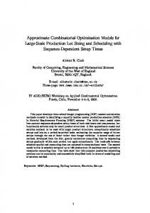
Figure 1: Geometrical representations for an N = 7 configuration: the permutation 1364725. In the top diagram, the TSP representation is shown. Note the dependence on boundary conditions and that there is a continuous path from one wall to the other. The second diagram interprets the displacement energy as bipartite matching: each line could be regarded as a spring pulling the relevant point to its sorted location. The final diagram is a different representation of the displacement energy as an assignment problem using just one set of nodes. In this representation, the permutation splits up into several separate pieces corresponding to its disjoint cycles.
The energy function for our second model, which we shall term the displacement energy due to its connection with the “total displacement” of R.W. Floyd[10], (0) is given as a sum of site distances from the sorted configuration Pi = i. ED (P ) =
N N 1 X 1 X (0) d(Pi , Pi ) = |Pi − i| 2N i=1 2N i=1
(3)
This form of cost function is familiar as an “assignment problem” [8]. The choice of distance measure relying on site differences is by no means unique. Many other ways of defining the distance between configurations are possible. For example, in the physics literature, an overlap based on counting similar links is common [11]. Another overlap (that happens to yield a tractable model [12]) is based on the matching problem and is determined by counting the number of sites that are in their correct relative positions. The different cost functions can be interpreted geometrically as illustrated in figure 1. For the permutation, 1364725 with N = 7, used as the example in the figure, the energies may be computed as: ET SP
These expressions and the diagrams in the figure make it clear that the energy may be computed as a sum over runs (either ascending or descending) in the case of the TSP energy, and as a sum over cycles in the case of the displacement energy. A run is the term used in the combinatorial literature for a subsequence of adjacent elements that are in sorted (or antisorted) order. For the TSP energy each contribution is the difference between the maximum and minimum value contained in the run. However, the contribution of each cycle to the displacement energy is not usually a single term (for more complex permutations than that shown in the figure) and it is necessary to look at runs within a cycle.
3
Relation between Models
The energy spectra of ET SP and ED are identical. That is, there is a one-one map between the full list of energies for all states computed with ED and the list computed with ET SP . Of course there is a shuffling in the way the states are associated with energies. For example, figure 2 shows the spectrum of the N = 4 model, with states labeled for each energy function. For many, but not all of these N = 4 states, the energy is the same whether evaluated with the TSP or the displacement energy. The proportion of states with invariant energy decreases at larger N . There are many degeneracies between energy levels: in the figure there are a 9-plet, a 7-plet, a 4-plet and a triplet besides the singlet ground state (which is always unique) that together make the 4! = 24 states. In appendix B we list the multiplicity structure for small values of N . This information might be expected to lead to an expression for the partition function. However, we have been unable to obtain a general formula for these multiplicities and according to Knuth[5], the generating function does not appear to have a simple form.
3.1
Mapping between Models
To demonstrate the relation between the two models formally, we present a mapping between the states P → P ′ , (in fact a permutation in the state space) that has the property that ED (P ) = ET SP (P ′ ). The mapping relies on the representation of the state P in terms of a permutation of the ordered state (1, 2, 3 . . . N ) using the cyclic representation. This mapping is well-known and is for example described in Knuth [13]. We write any permutation in terms of M distinct cycles (singleton cycles included explicitly). Each cycle is labeled by a superscript j and contains mj elements in the cycle as: M M M (i11 i12 i13 . . . i1m1 )(i21 i22 i23 . . . i2m2 ) . . . (ij1 ij2 ij3 . . . ijmj ) . . . (iM 1 i 2 i 3 . . . i mM )
(5)
We fix the freedom available in the way the cycle form is written by requiring that: • The largest element appears at the start of each cycle: ij1 > ijk for all other k in the cycle k = 2, 3 . . . mj . > ij1 • Cycles appear in the order determined by their first elements: ij+1 1 for j = 1, 2 . . . (M − 1). 5
Figure 2: Spectrum for N = 4. The multiplets and their energies are shown in the centre the left column shows the states according to the TSP energy and the right column shows them according to the displacement energy. States that are marked with a “∗” take different energies depending on the energy function used.
6
Note that this is slightly different from the convention defined by Knuth. The action of this permutation on the ordered state (1, 2, 3 . . . N ) is to take the value ijk to ijk+1 (or cyclically). The resulting permutation is the original state P of the map. The state P ′ obtained from the map is given simply by removing brackets from the definition of the element (5) above and regarding the list of numbers as a permutation. For example with N = 4, the cyclic form (1)(423) takes 1234 to 1342. Thus P = 1342 and P ′ = 1423. In this case, both P and P ′ lie in the same multiplet according to either the TSP or displacement energy. This is not the case for P = 3412 and P ′ = 3142 that appear at the top of figure 2 and correspond to the cyclic form (31)(42). Nonetheless, ED (3412) = ET SP (3142). The displacement energy in the state P is given by a sum over cycles as: ED =
The TSP energy can be evaluated in the state P ′ to obtain three terms, one from the elements at the end of the original sum in (2), one from the contribution of each cycle, and a term corresponding to the intercycle contributions. ET SP
=
M−1 1 1 1 X j M d(ij+1 (i − imM ) + 1 , i mj ) 2N 1 2 j=1
The cycle sums appearing in (6) and the last term in (7) are identical except for one additional term in the first equation. The total difference between the energies is given by: ET SP − ED =
M−1 M 1 X j+1 1 1 1X j j ) + (i1 − iM | − |i − i |i − ijmj | mM mj 2N 2 j=1 1 2 j=1 1
(8)
Now, by using the requirements on ordering of the ijk ’s stated above, we find that the modulus signs may be removed in each sum and the total vanishes. This does not occur for other choices of distance function, but does continue to hold for the model based on real numbers rather than integers. The map is invertible due to the requirements listed above. Note that the map must leave the ground state unchanged. However, the multiplet structure is not preserved, states that appear in a certain multiplet according to one energy function may appear in a different multiplet according to the other energy function. This can be seen in the case of N = 4 as the states marked with a “∗” in figure 2. Several distinct versions of the map exist, based on different conventions for the way the cycle form is written. An approach to understanding the symmetries of the system would be to combine a map and the inverse of a different version. We do not consider this approach here since it takes us too far afield from the aim of the present paper.
7
3.2
Average Energy
Here we consider statistics of the energy (either TSP or displacement) spectrum: the average energy and its fluctuation. These are averages from a combinatorial point of view in which all states contribute equally; thermodynamically they are effectively at infinite temperature. An estimate of the large N behavior is most easily obtained by writing the TSP energy in terms of h∆i, the average distance between nodes: hET SP (N )i =
N 1 N 1 X h|Pi+1 − Pi |i ≈ h∆i = 2N i=0 2 6
(9)
Where the approximation consists in ignoring correlations between the distances between different pairs of nodes. In this case, the pairs can be imagined as two independent points thrown at random in the interval [0, N ], so the average distance between them is h∆i = N/3. A more formal P computation based on the displacement energy proceeds as follows, where P indicates a sum over all permutations. hE(N )i
=
N 1 X 1 X |Pi − i| N! 2N i=1 P
N
=
1 XX |Pi − i| 2N N ! i=1
=
N N (N − 1)! X X |k − i| 2N N ! i=1
P
(10)
k=1
The order of summation is exchanged in the second line after which the sum over permutations becomes simple since there are (N − 1)! permutations in which Pi takes a given value k. The resulting sum can be performed using standard techniques and a similar argument holds for the second moment. N2 − 1 6N (N + 1)(2N 2 + 7) (11) h(E(N ) − hEi)2 i = 180N 2 p The width of the energy distribution, h(E − hEi)2 i, scales as N 1/2 and therefore becomes relatively more peaked at large N . hE(N )i
4
=
Dynamics
Although the energy spectra of the two models is identical and the partition functions are the same, the models still have distinct properties. This would be apparent by studying the response to some external field that couples to states in the same way in each model. The displacement energy itself could be regarded as an example of this kind of additional term in the cost function.
8
However, in the context of this paper and the problem of sorting, the distinction is best studied by looking at the dynamical properties of the models. We only consider local dynamics: that is the basic moves are adjacent transpositions. Of course there is no physical basis to these models requiring locality, and in real sorting algorithms non-locality of the elementary moves is essential to obtain efficient sorting. Furthermore, we only consider a dynamics associated with the energy function - namely the Monte Carlo Metropolis algorithm. This is natural from a theoretical physics perspective (even though it does not correspond to any physical dynamics [14]), but algorithms that have much less clear relationship with the cost function are common in computer science. Indeed we could imagine a reasonable algorithm that selects random sites and transposes with the neighbor if they are out of order. The usual approach physicists have used to investigate computer science problems is to study the dynamical relaxation under local search algorithms [3]. From the physical point of view, the approach consists in studying the phase ordering kinetics after a deep quench [6]. 18
16
14
Energy
12
10
8
6
4
2
0 0
5000
10000
15000
20000 MC steps
25000
30000
35000
40000
Figure 3: Dynamical evolution of the energy according to zero temperature Monte Carlo using local moves. The curve that reaches a plateau is for the TSP energy and the other is for the displacement energy. Size N = 100. An average over 1000 different initial states is taken with error bars that are too small to be shown.
4.1
Zero Temperature Metropolis Algorithm
The Monte Carlo moves are local adjacent transpositions and at zero temperature this effectively constitutes a randomized steepest descent algorithm. The 9
Metropolis algorithm we shall use selects a trial site at random and transposes with its (right hand) neighbor provided this move reduces the energy (or does not change it). We perform numerical simulations starting from a random configuration which typically has energy very close to the average energy computed in section 3.2. Figure 3 shows the results of numerical studies of dynamics according to this algorithm. The two curves in the figure correspond to dynamics based on each of the energy functions we have defined. Starting from a randomly chosen initial state, the plot follows the evolution of the energy averaged over many choices of this initial state. This situation corresponds to a quench from very high temperature to zero temperature. The model based on the displacement energy evolves in the expected manner: the energy slowly reduces and eventually reaches the sorted ground state. The other model, based on the TSP energy starts with a similar initial energy then rapidly reduces to a plateau value at which level it continues indefinitely. No further decrease in energy is evident, even for much longer runs, and the energy never arrives at the sorted ground state. This behavior can be improved somewhat by using simulated annealing but it remains extremely slow and still tends to get stuck. N=100 N=200 N=400 N=800 N=1600 N=3200
0.1
Energy/N
0.01
0.001
0.0001 0
1
2
3 4 Time (MC steps/N^2)
5
6
Figure 4: Scaling of the dynamical evolution of the displacement energy according to zero temperature Monte Carlo using local moves. Six size systems from N = 100 to N = 3200 are shown with axes scaled to demonstrate data collapse. The energy axis is scaled by 1/N and is plotted logarithmically. The time axis is scaled by 1/N 2 . An average over 1000 different initial states is taken with errors that are too small to see on the figure.
10
7
4.2
Timescales for Energy Decay
According to figure 3, the displacement energy appears to reduce at an exponential rate. The log-log plot (not shown) is only able to substantiate this for the first part of the decay. The quality of this initial exponential decay, and the form of the subsequent deviations from this form are shown in figure 4. Within the initial exponential decay region it is possible to measure the N dependence of the exponential timescale. At short times this characteristic time scales as N 2 (fits using times up to order N 2 give the exponent with accuracy ∼ 0.1%, and value tending to 2.0 as fewer points are taken), so the time axis of the figure has been scaled as t/N 2 in order to collapse the data in the initial region. The deviation from exponential form and absence of data collapse in the later part of the data is a finite size effect. With the help of small quantities of data for very large sizes up to N = 105 , careful measurements of the time required to reach fixed values of E/N can be made. The way these times scale with N shows a consistent trend towards an exponent of 2.0 at larger N . 0.17 N=100 N=400 N=1600 0.16
Energy/N
0.15
0.14
0.13
0.12
0.11
0.1 0
5
10 Time (MC steps/N)
15
Figure 5: Scaling of the dynamical evolution of the TSP energy according to zero temperature Monte Carlo using local moves. Three size systems, N = 100, N = 400, and N = 1600 are shown with axes scaled to demonstrate data collapse. The energy axis is scaled by 1/N . The time axis is scaled by 1/N . An average over 1000 different initial states is taken with errorbars that are the size of the marks. Certainly for any size that can be simulated, the total time to arrive at zero energy is affected by the finite size effects and has a scaling exponent larger than 2. Not surprisingly, the resulting sort is rather slower than achieved with
11
20
standard sorting algorithms that have best case behavior increasing as N log N . For the TSP energy, figure 5 shows a scaled plot for different size systems. In this case the time is only scaled by a factor of 1/N and the energy axis is not logarithmic. The stability of the plateau energy is very clear in this figure. A detailed investigation finds that after the effect of finite size effects are removed, the per site energy on the plateau is ET SP /N = 0.1092 ± 0.0001. The fact that the evolution timescales of the TSP and displacement models are respectively N and ∼ N 2 indicates another surprising distinction between the dynamics of the two models. 0.45
0.4
0.35
0.3
C(r)
0.25
0.2
0.15
0.1
0.05
0 0
5
10
15
20
25 r
30
35
40
45
50
Figure 6: The spatial correlator for configurations chosen in the plateau region (after 20000 steps on figure 3, though the form is the same for all configurations on the plateau) of the evolution of the TSP energy. Size N = 100 averaged over 1000 different initial states.
4.3
Spatial Correlations
Throughout this work we have implicitly considered the indices to form a line. In this section we consider correlations along this line and refer to such correlations as spatial. Studying the evolution of these correlators may illuminate the dynamical properties of the model since dynamical lengthscales may appear. By analogy with the definition of the distance metric (1), we define the spatial correlator at distance r as: N −r X 1 |Pi+r − Pi | C(r) = N (N − r) i=1
12
(12)
Up to terms relating to boundary conditions, C(1) is nothing other than the TSP energy. A small value of C signifies a strong correlation, and in the fully sorted state it grows linearly C(r) = r/N . From arguments similar to those used to derive the average energy, it can be shown that the correlator takes a constant value of 1/3 when averaged over randomly chosen configurations (more precisely, hC(r)i = (N + 1)/3N ; r > 0). In the figures to follow, we only show C(r) up to values of r < N/2. This is because for larger r, only a small number of pairs appear in the sum (12) and the indices of these pairs are often near the boundaries, thus making this region excessively dependent on boundary effects. As the configuration evolves according to the TSP model, the spatial correlator remains similar to its initial constant value 1/3 corresponding to the initial random configuration, but some structure develops at small r. Once the plateau is reached, there is no further change in the spatial correlator and figure 6 shows its final form. The non-trivial structure has a clear size, of less than 10 units, and neither the size scale nor the shape of the structure depend on N . This scale indicates the distance over which ordering can take place according to the TSP dynamical process. The mechanism that blocks further growth of the order beyond this scale is discussed below. 0.5 0.45 0.4 0.35
C(r)
0.3 0.25 0.2 0.15 0.1 0.05 0 0
5
10
15
20
25 r
30
35
40
45
Figure 7: The evolution of the spatial correlator for the displacement energy. Size N = 100 averaged over 1000 different initial states. In order of increasing slope the lines are for configurations taken every 10000 Monte Carlo steps after the start of the simulation. There is no change after 40000 steps. In the case of the displacement energy, the correlator evolves as shown in figure 7. Here, no detailed structure ever appears, and the correlator is always a straight line with a gradient that smoothly evolves towards the steepest slope corresponding to the final sorted ground state. There is no characteristic length13
50
scale over which ordering takes place and then grows. It would rather appear that the system becomes organized on all scales simultaneously.
4.4
Time Correlations
In order to investigate correlations between configurations at different times, we use the same overlap that was employed for the displacement energy. C(t, t′ ) =
N 1 X |P (t)i − P (t′ )i | 2N i=1
(13)
Other possibilities are certainly possible. For example, an overlap based on matching counts the number of positions where the number has not changed. The graphs based on this choice do not convey any significantly different information from those given below. 0.1 0.09 0.08 0.07
C(t,tw)
0.06 0.05 0.04 0.03 0.02 0.01 0 100
1000 log(t-tw)
Figure 8: Two-time correlators C(t, tw ) shown for different waiting times for the evolution according to TSP energy. Size N = 100 averaged over 1000 different initial states. Waiting time is zero for the top curve and increases by 200 in each lower curve until the bottom curve which is the same for any waiting time greater than 1000. This lowest curve indicates that aging does not occur. The simplest correlation to measure is against the completely sorted ground state. This is none other than the displacement energy itself, and was shown (for dynamics based on this energy) in figure 3. Another familiar comparison is against the initial state. For the dynamics according to the displacement energy, the correlation with the initial state disappears rapidly (within about 20N steps), and we do not show a figure in 14
this case. For the dynamics according to the TSP energy, we show in figure 8 the two-time correlators for different waiting time plotted against log(t − tw ) in the conventional manner. For tw = 0 the correlation against the initial state is included in this figure. We have drawn two-time correlators not because aging occurs in this model - it does not, but as a convenient way of demonstrating two features: that the configurations on the plateau retain some correlation with the original random state, and to show that evolution is not frozen on the plateau. With this aim, the waiting times shown in figure 8 are quite short. The final value of the tw = 0 curve (about 0.092) is much less than that associated with correlation between random configurations (1/6 in this case due to the factor of 2 in the definition (13)), indicating that not all information in the original configuration has been lost by the time the plateau is reached. This agrees with the result of the spatial correlation that indicates that only local modification takes place. The lowest two-time curve holding for all tw > 1000 (for size N = 100) corresponds to waiting times that have reached the plateau. This curve is not constantly zero as would be the case if there was no dynamics happening on the plateau. The configuration continues to evolve, though the energy does not change. However, the correlation is bounded: irrespective of how long after the waiting time, the correlator never rises above a certain value (about 0.021). This limiting value is independent of N . The reason for this behaviour is the limited size of the flat directions that are identified below.
3142
3412
4132
4312
3421
3241
4321
4231
Figure 9: Local minima for N = 4. The four states in the centre have TSP energy ET SP = 3 while those on the periphery have ET SP = 4. Local transpositions allow three possible moves between states and these are all shown for the local minima quartet.
15
4.5
Local Energy Minima
The fact that a simple algorithm such as zero temperature Monte Carlo is unable to find the ground state is hardly a surprise in optimization models. There are many statistical mechanical examples of this state of affairs, and the effect is usually ascribed to the features of the free energy landscape. In the K-Satisfiability problem the difficulty of finding the ground state via a local search procedure is due to the proliferation of states which trap the search into metastable phase. Eventually, a large fluctuation provides a means of reaching the ground state [15, 16]. However, in our TSP model the reason is more prosaic and the origin of the effect is due to the presence of stable local energy minima. In this respect, it is similar to the XOR-SAT model, that also suffers from such minima [2]. Though the two energy functions have matching energy levels they have very different energy landscape characteristics. The displacement version has no stable local minima, but the TSP version does. Moreover, these minima appear to proliferate as N increases and are never avoided. For small values of N the local minima of the TSP model may be found explicitly. No such minima exist for N = 3. For N = 4 there are four minima connected by Monte Carlo moves as shown in figure 9. Note that these minima are precisely the states that appear with a “∗” in figure 2, and indeed the energy assignments of figure 9 are inverted for the displacement energy, so in that case there are no local minima.
Figure 10: A schematic representation of the trapping configuration found on the plateau. The turning pairs are shown enclosed. This configuration could represent the N = 20 configuration: 5 9 17 14 11 6 8 20 16 15 7 4 1 3 10 12 18 19 13 2. For larger N , the trapping configurations appear as shown in figure 10. They consist of alternating ascending and descending runs separated by turning pairs. For an upper turning pair, each element of the pair is greater than either of the elements neighbouring the pair, with a similar definition for a lower turning pair. These trapping configurations found on the plateau, are slightly more ordered than random configurations that consist of ascending and descending runs separated by ordinary turning points. A turning point is a requirement on a subsequence of length 3, whereas a tuning pair is a requirement on a longer subsequence of length 4. The dynamical Monte Carlo process performs this small scale ordering (as observed in the spatial correlators) to arrive at the plateau configurations. The trapping configurations are stable local minima: flat directions correspond to the moves that interchange the two elements of the turning pairs, and all other transpositions raise the energy. The number of states in the trap is 16
therefore 2number of turning pairs . Since the number of turning pairs grows linearly with the size of the system, the size of the trap grows exponentially with N . In appendix C, an estimate for the number of turning points (same as the number of turning pairs) for plateau configurations is derived, so the exponential growth is approximately 2N/3 . Of course, many different traps exist, each with this typical size. The picture of the trapping configurations in figure 10 makes the turning pairs appear like domain walls. This is a reasonable interpretation since the bulk part of the TSP energy has two different minima with ascending and descending order and it is these phases that are separated by the turning pairs. The boundary conditions raise the degeneracy of the sorted and antisorted phases, but this effect never comes into play here since the domain walls are frozen and do not move after the initial relaxation. The local minima provide a basis for attempting to understand the value of the plateau energy observed under the dynamics above. A rather naive argument given in appendix C, based on characterizing the typical length of ascending or descending runs in the permutation defining the local minimum state gives the per site value of 1/10. This should be compared with the numerical value of ET SP /N = 0.1092 ± 0.0001 found in section 4.2. 7
6
5
Energy
4
3
2
1
0 0
0.2
0.4 0.6 Interpolation parameter p
0.8
Figure 11: The final (plateau) energy of the interpolating Hamiltonian. For the ordered model, size N = 40, with error bars indicating an average over 1000 random initial states. Note the ledge near p = 1, and that only for p = 1 does the algorithm succeed in finding the zero energy state.
17
1
4.6
Interpolating Model
Given the rather different dynamic properties of the two models, it is natural to consider the behavior of models interpolating between them. The interpolating Hamiltonian is: E(p) = (1 − p)ET SP + pED (14) where p is a parameter in (0,1). The average energy (in the combinatoric sense at infinite temperature) is independent of p. All other quantities, such as the energy of individual states and the degeneracy pattern are different from either of the models previously discussed. Depending on the value of p, the dynamics is expected to be more like one or other of the two lines shown in figure 3. One might hope for a transition to take place for some intermediate value of p, but in fact the dynamics reaches a plateau for any p < 1. Figure 11 shows how the energy value of the plateau varies with p. For small N this curve is composed of a series of steps, ending in a horizontal ledge near p = 1. For larger N the curve becomes smooth and the width of the ledge shrinks, eventually the curve becomes a sawtooth. The question arises as to why stable local minima appear even for an infinitesimal perturbation away from the displacement energy. Consider the state corresponding to the completely reversed permutation (with the central two elements transposed in the case of N even). The displacement energy of this state is flat with respect to any of the local moves, though a series of moves will eventually lead to a lower energy state. On the other hand the same state is part of a local minimum quartet with respect to the TSP energy. An infinitesimal addition of the TSP component is therefore sufficient to make the state a local minimum, albeit with infinitesimally small barriers. Although this argument correctly describes the reason that trapping can take place for p so close to 1, the identification of completely reversed states as being responsible is incorrect since their energy is considerably higher than the plateau.
5
Conclusion
Considering statistical mechanical models based on states that are permutations of numbers, we have demonstrated a relationship between two models with distinct energy functions. Statically their partition functions are identical since the energy spectrum is the same. Dynamically there are substantial differences since one model has local energy minima and the other does not. This strange situation, that models with identical static properties have distinct local dynamics, is not a paradox. In this case it is clearly due to the shuffling of states that modifies the energy landscape by rearranging the energies of states that are close to each other. The static analysis showed that the energy spectrum was the same by demonstrating a one-to-one map relating states with the same energy in each model. This map continues to hold for the more general model based on real numbers rather than integers. Dynamically, we simulated a deep quench and showed that the energy decay proceeds in a completely different way in each of the two models. For the
18
displacement model, no dynamical lengthscale appears as the system is reorganised. Characteristic timescales do appear and vary as N 2 , though with strong finite size effects. For the TSP model, there was rapid (timescale varying as N ) decay to a plateau as a result of reorganisation over small spatial scales of size less than 10 units, that did not completely destroy the corelation with the initial state. Evolution continued to occur on the plateau, but was limited in range. This was interpreted in terms of trapping configurations with turning pairs. Flat movement within the trap was still possible between about 2N/3 local minima states. Optimization problems of most interest, such as K-Satisfiability, are much richer than the models presented here. Nevertheless, in the context of the one parameter family of interpolating models, we have shown that our simple local search procedure exhibits a transition (at the very edge of the interpolation region) from being able to sort the numbers to becoming trapped by local minima. We hope that these models provide a simple arena for studying the general question of the role of the energy landscape in the performance of local search algorithms.
19
A
Appendix: Model based on Real Numbers
Instead of the integer model discussed in the text, this more general model is based on the set of N real numbers xi , i = 1, 2 . . . N , with each xi in the range [0, N + 1]. Without any loss of generality, we take the xi ’s to be ordered (xi < xj for all i < j) as this makes the identity permutation of the indices correspond to the lowest energy, or sorted state. The xi ’s should be regarded as quenched random variables, and for this reason the model might be regarded as a disordered model in contrast to the integer ordered model. The disorder however, is not of the independent variety that has been considered for both assignment and TSP problems using a replica approach in [8, 17], but rather corresponds to Euclidean distances in one dimension. Here, the replica approach becomes intractable since the average over disorder couples sites. For the disordered model, the definitions of the two energy functions remain exactly as given on the first lines of equations (2) and (3), however the distance function is replaced by: d(Pi , Pj ) = |x(Pi ) − x(Pj )|
(15)
Irrespective of the choice of x’s, there are degeneracies in the spectrum, but not to the extent found in the ordered model. For example, for N = 4, the disordered model has energy levels with multiplicities (9,4,3,3,1,1,1,1,1). In the ordered model these combine to give (9,7,4,3,1). The mapping between the energy levels according to each model continues to hold, however there is a small difference in the moments. Here the moments are defined after additional averaging over the x’s. The mean energy is the same as in the ordered model by design - indeed it was this criterion that selected the range of the xi ’s to be [0, N + 1]. The second moment is however slightly larger than quoted in (11). h(E(N ) − hEi)2 i =
(N + 1)2 (3N 2 + 10N + 2) (N + 2)180N 2
(16)
Even for individual instances of the disordered model, similar dynamical behaviour to that described in the text for the integer model is observed. After averaging over realizations of the xi ’s, the similarity becomes even closer.
B
Appendix: Multiplicities of Degeneracies
The multiplicities are most easily obtained using the displacement energy ED This may be evaluated for every permutation and DN (E) denotes the number of times that displacement E appears. For small N (up to N ≈ 16), it is straightforward to numerically enumerate these coefficients, and the first few are given in the table below.
20
N 1 2 3 4 5 6
D(0) 1 1 1 1 1 1
D(1) 0 1 2 3 4 5
D(2) 0 0 3 7 12 18
D(3) 0 0 0 9 24 46
D(4) 0 0 0 4 35 93
D(5) 0 0 0 0 24 137
D(6) 0 0 0 0 20 148
D(7) 0 0 0 0 0 136
D(8) 0 0 0 0 0 100
D(9) 0 0 0 0 0 36
The usual arguments intended to lead to recurrence relations that would relate DN +1 (E) to sums of DN (E ′ ) are not helpful in this case. Although there are some relations based on a sum over partitions of ES , these are only valid in the region below the diagonal of the table. The problem appears to be non-trivial and indeed, according to Knuth[5], the generating function does not appear to have a simple form.
C
Appendix: TSP Plateau Energy
The average TSP energy is estimated after the effect of the Monte Carlo moves. It is convenient to evaluate the TSP energy by summing contributions from ascending and descending runs, rather than from adding each individual term which leads to many cancellations. The theory of runs of this kind is presented in [18], but very little of the general development is necessary here. The main property we use is that their endpoints are characterized by turning points in the permutation sequence. We assume that N is large and only consider leading terms. hET SP i ≃
N 1 X 1 h|Pi+1 − Pi |i ≈ hsih∆i 2N i=0 2N
(17)
Where hsi is the average number of runs, and h∆i is the average (absolute) change between the start and end of the run (∆ = d(Pstart , Pend )). The first approximation in this approach is to ignore the correlations between the number of runs and the value of ∆ for that run in the formula above. To illustrate this form, let us use it to reproduce the average energy of a random configuration. In that case, hsi = 2N/3, since by considering sets of three adjacent points, the central one has a maximum or minimum value in 4 out of the 6 equally likely orderings. To deduce h∆i we consider the average value taken at upper turning points separating runs. Since hmax(P1 , P2 , P3 )i = 3N/4 and a symmetric result for the minimum, h∆i = N/2. Combining these results in equation (17) reproduces hET SP (N )i = N/6 as was derived in the text by considering contributions from all neighboring pairs. An estimate of the value of the average in the plateau is obtained by taking into account the effect of the Monte Carlo moves. We consider a subsequence of four points and look at the effect of a transposition on the central pair of the four, in all 24 possible orderings. The four points are labeled 1234, but this only signifies their relative magnitude. Table 1 indicates whether the transposition causes a positive, negative or zero change in energy and lists the change in number of (internal) maxima or minima. 21
P 1234 2134 1324 1243 2143 3214 3124 2314
∆E + + + + 0 0 -
∆s 2 1 -2 1 0 0 0 -1
P 1432 1423 1342 4231 3241 4132 3142 4321
∆E 0 0 +
∆s 0 -1 0 -2 -1 -1 0 2
P 4312 3421 3412 4213 4123 2431 2341 2413
∆E + + + 0 0 0 0 -
∆s 1 1 0 0 0 0 0 0
Table 1: Effect of transposing central pair of 4 points. ∆E indicates the sign of the energy change as a result of this move. ∆s shows the change in number of (internal) turning points.
Using this table, we find that moves that do not change the energy do not alter the number of runs. Moreover, there are six configuration that both reduce the energy and number of runs. These are the pair 1324, 4231, and the quartet 2314, 1423, 3241, 4132. If we take their naive weights from the initial random configuration, then such transpositions for every pair of adjacent points leads to an average reduction in hsi of 2 × N × 2/24 + 1 × N × 4/24. So the final value after one Monte Carlo sweep is hsi = N/3. The argument for the average value at a maximum is extended from 3 (given in the example above) to 4 points, where it reproduces the 3 point case when all contributions are included. However, some of these contributions are removed by the Monte Carlo move (we only include those configurations with ∆E ≥ 0 in table 1) resulting in h∆i = 3N/5. Overall we obtain the estimate hET SP (N )i = 1/2N × N/3 × 3N/5 = N/10, to be compared with the numerical value of E/N = 0.1092 ± 0.0001. The approximations in this approach are quite drastic. First we ignored correlations between the number of runs and the value of ∆ for that run in formula (17). Then we just looked at the effect of one Monte Carlo sweep, used naive weights and ignored any influence of one Monte Carlo move on another. It is therefore surprising that we obtain such a reasonable estimate. Indeed, numerical studies show that the estimates of both hsi and h∆i are incorrect by about 10%.
22
References [1] O.C. Martin, R. Monasson and R. Zecchina. Theoretical Computer Science 265, 3-67 (2001). arXiv:cond-mat/0104428. [2] S. Cocco, R. Monasson, A. Montanari and G. Semerjian. Approximate analysis of search algorithms with “physical” methods. arXiv:cs/0302003. [3] P. Svenson and M.G. Nordahl. Relaxation in graph colouring and satisfiability problems. Phys. Rev. E 59, 3983 (1999). arXiv:cond-mat/9810144. [4] A. Percus. The Traveling Salesman and Related Stochastic Problems. Doctoral Thesis University Paris 6. (1997) arXiv:cond-mat/9803104. [5] D.E. Knuth. The Art of Computer Programming: Vol 3, Sorting and Searching. Addison Wesley 2nd Edn (1998). [6] A.J. Bray. Advances in Physics 43, 357 (1994). [7] P.J. Cameron. Combinatorics: Topics, Techniques, Algorithms. Cambridge University Press (1994). [8] M. M´ezard and G. Parisi. J.Physique Lett. 46, L771-L778 (1985). [9] Y. Fu and P.W. Anderson. J.Phys.A 19, 1605-1620 (1986). [10] The total displacement is introduced as an exercise (5.1.1 ex 28), ascribed to R.W.Floyd in reference [5]. [11] S. Kirkpatrick and G. Toulouse. J.Physique 46, 1277 (1985). [12] The generating function for the matching problem is given in [5]. [13] D.E. Knuth. The Art of Computer Programming: Vol 1, Fundamental Algorithms. Addison Wesley 2nd Edn (1998). Section 1.3.3 pg 178. [14] M.A. Novotny. A tutorial on advanced dynamic Monte Carlo methods for systems with discrete state spaces. arXiv:cond-mat/0109182. [15] G. Semerjian and R. Monasson. Relaxation and Metastability in the RandomWalkSAT search procedure. Phys. Rev. E67, 066103 (2003). arXiv:cond-mat/0301272. [16] W. Barthel, A.K. Hartmann and M. Weigt. Solving Satisfiability Problems by Fluctuations: the dynamics of local search algorithms. Phys. Rev. E67, 066104 (2003). arXiv:cond-mat/0301271. [17] M. M´ezard and G. Parisi. J.Physique 47, 1285-1296 (1986). [18] F.N. David and D.E.Barton. Combinatorial Chance. Griffin (1962). Chapter 10.