Two-field description of chaos synchronization in diode lasers with ...

PHYSICAL REVIEW A 72, 043818 共2005兲

Two-field description of chaos synchronization in diode lasers with incoherent optical feedback and injection

1

David W. Sukow,1,* Athanasios Gavrielides,2 Thomas Erneux,3 Michael J. Baracco,1 Zachary A. Parmenter,1 and Karen L. Blackburn1

Department of Physics and Engineering, Washington and Lee University, 116 North Main Street, Lexington, Virginia 24450, USA 2 Air Force Research Laboratory, Directed Energy Directorate AFRL/DELO, 3550 Aberdeen Avenue SE, Kirtland AFB, New Mexico 87117, USA 3 Université Libre de Bruxelles, Optique Nonlinéaire Théorique, Campus Plaine, Code Postal 231, 1050 Bruxelles, Belgium 共Received 14 July 2005; published 24 October 2005兲 Synchronized chaotic dynamics are investigated theoretically and experimentally in a system of unidirectionally-coupled semiconductor lasers subject to delayed, polarization-rotated optical feedback and injection. Experimental data in the time and frequency domains demonstrate chaos synchronization with a lag between transmitter and receiver equal to the injection time, also known as driving synchronization. The natural polarization mode of the transmitter is shown to synchronize most efficiently to the orthogonal state of the receiver which is being injected. A full two-polarization model is used for both lasers, and is in good agreement with polarization-resolved experimental measurements. DOI: 10.1103/PhysRevA.72.043818

PACS number共s兲: 42.65.Sf, 42.55.Px, 05.45.Xt

I. INTRODUCTION

Chaos synchronization has been studied extensively for semiconductor laser 共SL兲 systems because of their interest for optical communication systems. Chaos synchronization on unidirectionally coupled semiconductor lasers has been found in optical injection systems 关1兴, optical feedback systems 关2,3兴, optoelectronic feedback systems 关4,5兴, and systems of two mutually coupled semiconductor lasers 关6,7兴. In several experiments, it was shown that chaos synchronization can exhibit perfect synchronization, as expected, but driving synchronization as well. If a master laser subject to a delayed optical feedback injects its light into a slave laser of similar wavelength, perfect chaos synchronization between master and slave lasers is possible if the injection and feedback rates are comparable. On the other hand, if the injection rate is much larger than the feedback rate, a driven response is observed where synchronization occurs with the delayed injected signal rather than with the chaotic oscillations of the master 关3兴. An all-optical system which is dynamically equivalent to the optoelectronic feedback system is the incoherent feedback system 关8兴. But driving synchronization has never been observed for the optoelectronic feedback system 关9兴, whereas it was observed for the incoherent feedback system 关10兴. However, extensive simulations of an incoherent feedback model involving only one polarization field 关11兴 indicate that driving synchronization is not possible. This suggests that the one-polarization model might be too simple to describe the observed synchronization dynamics. In this paper, we employ a more realistic model where the two polarization fields are taken into account 关12,13兴. Recent numerical work using such a model has demonstrated both synchronization solutions in the incoherent optical feedback system 关14兴,

*Electronic address: [email protected] 1050-2947/2005/72共4兲/043818共6兲/$23.00

though the perfect synchronization solution occupies a relatively narrow region of parameter space. Previous experimental studies have considered singlemode diode lasers subject to incoherent optical feedback in several configurations 关13,15,16兴. The system we have studied is illustrated schematically in Fig. 1. This becomes the chaotic transmitter in our synchronization work presented here. It consists of a laser in an external cavity and intracavity devices that rotate the polarization state of the delayed optical feedback, adjust the feedback strength, and sample the output. A detailed description of our experimental, theoretical and numerical results of this system has been published recently 关17兴. In particular, we show that the extended model that takes account of both polarizations describes the experimental results very well, and under general assumptions it can be reduced to the usual incoherent model. Under these assumptions the two polarization model exhibits synchronization between the two modes as we have experimentally observed. In addition, we have analyzed the steady states and have studied their stability. In this paper we first discuss the extension to the full model of transmitter and receiver diode lasers in Sec. II along with numerical results that show the synchronization of the intensities of the two lasers. Experimental results are then discussed in Sec. III, followed by a summary and an Appendix delineating the synchronization equations.

FIG. 1. Schematic diagram of a laser with delayed incoherent optical feedback. 043818-1

©2005 The American Physical Society

PHYSICAL REVIEW A 72, 043818 共2005兲

SUKOW et al. II. SYNCHRONIZATION MODEL

The model that we use to examine synchronization of the receiver to the transmitter is the full model in which the chaotic wavefront of the transmitter is obtained by the delayed and polarization-rotated feedback 关14,17兴. Furthermore, part of the rotated feedback is injected into the receiver. We do not require terms for multiple external cavity roundtrip reflections for the transmitter, because our cavity configuration extinguishes them. The equations describe the fields E1, E2, and the carrier density N for each laser. The transmitter and receiver variables are denoted by superscripts t and r, respectively, giving the equations dEt1 = 共1 + ia兲NtEt1 , dt

共1兲

dEt2 = 共1 + ia兲共Nt − ␤兲Et2 + ␩te−i共␻1␶+␾e兲Et1共t − ␶兲, dt

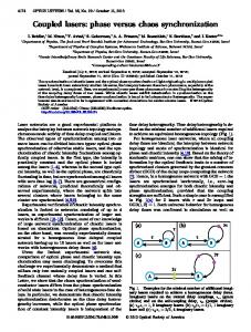
共2兲 FIG. 2. Time series of the chaotic waveform of the horizontal polarization of the transmitter It1.

t

T

dN = P − Nt − 共1 + 2Nt兲关兩Et1兩2 + 兩Et2兩2兴, dt

共3兲

dEr1 = 共1 + ia兲NrEr1 , dt

共4兲

the two polarizations and using ␥ p = 5 ⫻ 1011 s−1 for the cavity lifetime at ␭ = 1 ␮m leads to ⍀ ⬃ 1. However, the approximation ⍀ Ⰶ ␤ will be employed. We assume that otherwise all the remaining laser parameters are identical. In the Appendix, we obtain the approximation

dEr2 ¯ = − i⍀Er2 + 共1 + ia兲共Nr − ␤兲Er2 + ␩re−i共␻1␶c+␾e兲Et1共t − ␶c兲, dt

¯

Er2 =

共5兲 T

dNr = P − Nr − 共1 + 2Nr兲关兩Er1兩2 + 兩Er2兩2兴. dt

共6兲

In these equations, t = ␬t⬘ and ⍀ = ⍀⬘␬−1 where ␬−1 is defined as the cavity lifetime. Besides the feedback parameters which can be controlled, the important parameters are T ⬃ 103 defined as the ratio of the carrier density and cavity lifetimes, the linewidth enhancement factor a ⬃ 2 – 5, and the pump parameter above threshold P ⬃ 0.1– 1. We also note that the value of the differential gain ␤ ⬃ 0.1 is relatively large compared to the relaxation oscillation frequency ␻ ⬃ 0.03. We have verified that the parameters used in Refs. 关13,14兴 reformulated in dimensionless form are of the same order of magnitude as the ones used here. In Refs. 关13,14兴, the two polarizations are assumed to exhibit different gain coefficients while we assume same gain but different damping rates. The first three equations describe the transmitter. We have assumed that the reinjected, polarization-rotated feedback in the transmitter has the same frequency and we have set ␻t1 = ␻t2. However, this is not the case in the receiver and indeed as we have found experimentally there is a detuning between the injected field from the transmitter and the field of the receiver. In addition, this detuning can be controlled by adjusting the temperature of the receiver by ±5 ° C. This corresponds to as much as ±1 nm and we will see that it can affect the strength of the injection. A quick estimate shows that taking ⌬␭ = 1 nm for the wavelength separation between

␩re−i共␻1␶c+␾e兲 t E 共t − ␶c兲. i⍀ + 共1 + ia兲␤ 1

共7兲

Equation 共7兲 implies that there is driving synchronization between the vertical polarization of the receiver and the rotated horizontal polarization of the transmitter delayed by the path from the master laser to the slave laser. The question of whether the horizontal polarization of the receiver is also synchronized to the injected field from the master, i.e., the relationship between Er1共t兲 and Et1共t − ␶c兲, cannot be answered analytically. This synchronization is only possible through the mediation of the carriers and will be examined numerically. We compute numerically the synchronization of the receiver to the transmitter for two identical devices that are characterized by the following parameters. Pump P = 0.5, a = 2.0, the ratio of the carriers to the cavity lifetime T = 1000, feedback delay ␶ = 1200, external delay from the transmitter to the receiver of ␶c = 1400, and differential loss of ␤ = 0.1. The transmitter has a feedback ␩t = 0.134 and is operating in the chaotic regime. The receiver is assumed to have a larger feedback rate ␩r = 0.234. Figure 2 shows a segment of the time series of the horizontal intensity It1 versus the normalized time to the dimensionless relaxation oscillation frequency ␻ = 冑2P / T. The lifetime of the cavity is assumed to be ␥ p = 2.43⫻ 1011 s−1. The chaotic time series contain pulses separated by about the external cavity round trip time which is ␽ = ␻␶ ⯝ 37.95, and bursts separated by about 300–400 time units of a slower frequency. We introduce the correlation between two signals as

043818-2

PHYSICAL REVIEW A 72, 043818 共2005兲

TWO-FIELD DESCRIPTION OF CHAOS…

FIG. 3. Correlation of the horizontal polarization of the transmitter It1 with the vertical polarization of the receiver Ir2 as a function of the delay.

冕 冋冕 冕

S1共t兲S2共t − s兲dt

C共s兲 =

S21共t兲dt

S22共t兲dt

册

. 1/2

共8兲

The correlation between the horizontal polarization intensity of the transmitter It1 and of the receiver vertical polarization intensity Ir2 is shown in Fig. 3. The maximum correlation corresponds to a delay of 44.09 and corresponds very well to the normalized delay from receiver to transmitter of ␽c = ␻␶c ⯝ 44.27. At this delay the correlation is maximum at 0.896. The type of synchronization with the delay equal to the time of flight from the transmitter to receiver is identified as driving synchronization. This contrasts with perfect synchronization where the delay between the transmitter and the receiver signal is equal to the difference ␶c − ␶. This is a good verification of Eq. 共7兲. Figure 3 also shows that there are multiple peaks separated by about 40 time units corresponding to the external delay of the transmitter and several peaks at multiples of 250– 350 units that correspond to the low frequency envelope of the rapid oscillations in Fig. 2. Figure 4 shows a visual correlation by a scatter plot of the time series of It1 versus shifted Ir2. However, the correlation between It1 and Ir1 the natural polarization of transmitter and receiver is only 0.63 and corresponds to a delay of 43.56 at the maximum of the correlation. We also observed a slight difference between the delays 共It1 , Ir2兲 = 44.09 and 共It1 , Ir1兲 = 43.56 implying a difference on the order of 100 ps in real time. This observation qualitatively agrees with the experimental observations of a delay of 200 ps. Some of the fixed parameters need to be measured for a more quantitative comparison. We also find a correlation of 0.84 and a delay of 43.9 between the two intensity time series at the maximum of the correlation.

FIG. 4. Scatter plot of the transmitter horizontal polarization intensity versus the vertical polarization of the receiver.

lasers coupled unidirectionally. Experimental findings confirm that the two polarization states play a significant role in the nature and quality of the synchronization between transmitter and receiver. The experimental apparatus for synchronization via unidirectional injection consists of a transmitter laser that is driven into chaos by use of polarization-rotated, delayed optical feedback, and a receiver laser that is to be synchronized through unidirectional injection of the transmitter’s polarization-rotated beam. This is illustrated schematically in Fig. 5. Both lasers are of the same model 共Sharp LT024兲 but have slightly different nominal operating characteristics. The transmitter 共LD1兲 has a nominal wavelength of ␭1 = 782 nm and a solitary threshold of 45.6 mA; the receiver 共LD2兲 runs at ␭2 = 781 nm and a solitary threshold of 41.0 mA. For all experimental data presented in this section, LD1 is driven with a current of 64.02 mA and stabilized at a temperature of 16.02 ° C; LD2 is driven with a current of 60.07 mA and stabilized at a temperature of 16.01 ° C. The pump currents are chosen such that the relaxation oscillation frequencies of the two lasers are made to be as similar as possible. The quality of synchronization does tend to degrade noticeably with changes in pump current, which shifts the relaxation

III. EXPERIMENT

Building upon our previous studies of the two-field chaotic transmitter laser 关17兴, we now examine the case of two

FIG. 5. Schematic of the experimental setup for synchronization via unidirectional coupling.

043818-3

PHYSICAL REVIEW A 72, 043818 共2005兲

SUKOW et al.

oscillation frequency. However, variations in temperature 共thus wavelength, by at least ±1 nm兲 do not strongly affect the synchronization phenomena we observe, indicating that it is not critically dependent on wavelength matching between the two lasers. Chaos is induced in the transmitter laser using delayed optical feedback. The horizontally-polarized beam emerging from LD1 is collimated by a lens 共CL1兲 with numerical aperture of 0.47, passes through a plate beamsplitter 共BS, R = 30%兲, then enters a Faraday rotator 共ROT兲 whose input polarizer is removed. The beam’s polarization rotates 45°, and exits through the output polarizer with its transmission axis set at 45°. A rotatable linear polarizer 共POL兲 in the external cavity adjusts the beam’s intensity 共and thus the feedback strength兲. A partially reflecting mirror 共PM兲 reflects 30% of the beam, which then is rotated an additional 45° on the return pass through the rotator. This creates a verticallypolarized beam that is reinjected into LD1 and induces dynamical instabilities. Note that all multiple roundtrip reflections are extinguished, because vertically-polarized reflections from the laser’s facet are rotated 45° a third time, thus becoming perpendicular to the Faraday rotator’s output polarizer. The external cavity roundtrip length is 80.8 cm, with a roundtrip time ␶ext = 2.69 ns. For all data shown in this section, the external cavity transmission Text = 12.7%. The portion of the LD1’s output that is transmitted through the partial end mirror becomes the injection beam for synchronizing LD2. It enters a Faraday isolator 共ISO兲 whose input polarizer is oriented 45° relative to the horizontal 共parallel to the beam兲, rotates an additional 45° to vertical, and exits the isolator through the vertically-oriented output polarizer. It then strikes two high-reflectivity steering mirrors 共HR兲, reflects from a polarizing beamsplitter cube 共PBS兲, and couples into LD2 through a collimating lens 共CL2兲 identical to CL1. The injection path length from LD1 to LD2 is 140.1 cm, giving an injection time of ␶inj = 4.67 ns. Unidirectional coupling is ensured by the Faraday isolator. Accounting experimentally for all splitting and losses, the injection strength Tinj = 23.2%, again expressed as a fraction of LD1’s total output power. We remark that various injection strengths have been explored using a variable neutral density filter inserted into the injection arm, with similar results. The intensity dynamics of both LD1 and LD2 are sampled immediately after they emerge from their respective collimating lenses, by use of the plate beamsplitters 共BS兲, which direct 30% of the incident light to the detection arms. For both lasers, linear polarizers are inserted into the beam path to allow polarization-resolved detection, as the transmitted beams strike identical ac-coupled photodetectors 共PD1 and PD2兲 with detection bandwidths of 8.75 GHz 共Hamamatsu C4258-01兲. Neutral density filters 共not shown兲 attenaute both beams to limit the power incident on the detectors. The detected signals are amplified with ac wideband 共10 kHz– 12 GHz兲 microwave amplifiers 共AMP兲 with 23 dB gain, and then are displayed on either an rf spectrum analyzer 共Agilent E4405B, 13.2 GHz BW兲 or a high speed digitizing oscilloscope 共LeCroy 8600, 6 GHz analog bandwidth and 50 ps sampling interval兲. We use the fast oscilloscope to acquire simultaneous data sets from specific linear polarizations of the transmitter and

FIG. 6. Time series data showing synchronization via unidirectional coupling.

receiver lasers. The time series have lengths of 4000 points with a 50 ps sampling interval for a total duration of 200 ns. We then determine the maximum cross-correlation coefficient S between the pair using the time-shifted function S共⌬t兲 =

具P1共t兲P2共t − ⌬t兲典 关具P21共t兲典具P22共t兲典兴1/2

,

共9兲

where P1 and P2 are the transmitter and receiver powers, respectively, and ⌬t is the shift between the two time series at which the cross-correlation is calculated. Time series data are displayed in Fig. 6. For ease of visual comparison, we scale and shift the axes for each time series. All waves are scaled vertically by subtracting the mean and normalizing the standard deviation to unity, and the lagging wave of each pair is shifted horizontally by the ⌬t associated with the maximum cross-correlation. Figure 6共a兲 shows the synchronization between the horizontally-polarized mode of the transmitter and the vertically-polarized mode of the receiver 共the injected mode兲. The transmitter and receiver lasers are represented by the thick gray and thin black curves, respectively. The data appear very similar, supported by a maximum cross-correlation coefficient of S = 0.91 when ⌬t = 4.83 ns, a lag close to but slightly greater than the injection time ␶inj = 4.67 ns. Figure 6共b兲 shows the case for the horizontal modes of both lasers. Visually, the time series have more obvious differences, and this is supported by the lower maximum S = 0.75 when ⌬t = 5.03 ns.

043818-4

FIG. 7. Synchronization plots for unidirectional coupling.

PHYSICAL REVIEW A 72, 043818 共2005兲

TWO-FIELD DESCRIPTION OF CHAOS…

ACKNOWLEDGMENTS

This material is based upon work supported by the U.S. National Science Foundation under CAREER Grant No. 0239413. Acknowledgment also is made to the W.M. Keck Foundation for the partial support of this research. T.E. acknowledges the support of the Fonds National de la Recherche Scientifique 共FNRS, Belgium兲 and the InterUniversity Attraction Pole program of the Belgian government. APPENDIX: SYNCHRONIZATION

Consider the two lasers in a transmitter-receiver configuration. The transmitter laser equations are given by dEt1 = 共1 + ia兲NtEt1 , dt

FIG. 8. rf power spectral data for unidirectional coupling.

The same time series data are displayed in the form of synchronization plots in Fig. 7. Graphs 7共a兲 and 7共b兲 correspond to their counterparts in Fig. 6. In both cases the data clearly lie along diagonal, but the loss of synchronization quality between Fig. 7共a兲 and Fig. 7共b兲 is visibly apparent, with Fig. 7共b兲 displaying a significantly more dispersed ellipse. As a final experimental assessment of the synchronization between these two pairs of data, we consider the frequency domain as shown in Fig. 8. Once again, the first graph, Fig. 8共a兲, shows the relationship between the horizontallypolarized mode of the transmitter and the vertically-polarized mode of the receiver 共the injected mode兲. The power spectra of the transmitter and receiver lasers are represented by the thick gray and thin black curves, respectively. The frequency content of the transmitter is transferred to the receiver effectively. In contrast, the data shown in Fig. 8共b兲 reveal a far less efficient transfer between the horizontal modes of the transmitter 共thick gray curve兲 and the receiver 共thin black curve兲. The receiver’s power spectrum is much more suggestive of the broad relaxation oscillation signature, with only a portion of the transmitter’s frequency content transferred to it. This is consistent with the lower-quality synchronization obtained between these two modes.

共A1兲

dEt2 = 共1 + ia兲共Nt − ␤兲Et2 + ␩te−i共␻1␶+␾e兲Et1共t − ␶兲, 共A2兲 dt T

dNt = P − Nt − 共1 + 2Nt兲关兩Et1兩2 + 兩Et2兩2兴 dt

共A3兲

while the receiver laser equations are of the form dEr1 = 共1 + ia兲NrEr1 , dt

共A4兲

dEr2 = − i⍀Er2 + 共1 + ia兲共Nr − ␤兲Er2 + ␩re−i共␻1␶+␾e兲Et1共t − ␶c兲, dt 共A5兲 T

dNr = P − Nr − 共1 + 2Nr兲关兩Er1兩2 + 兩Er2兩2兴. dt

共A6兲

In the case of the receiver, we noted experimentally a significant detuning between the injection field of the transmitter and the orthogonal field of the receiver ⍀ = ␻t1 − ␻r2 ⫽ 0. For numerical simplicity, we have assumed zero detuning. Typical values of the parameters are P = 0.5,

T = 103,

a = 2,

␶ = 1200,

␶c = 1400, 共A7兲

IV. SUMMARY

In summary, we have presented analytical, numerical, and experimental results that explore the nature of chaos synchronization in a system of unidirectionally-coupled semiconductor lasers subjected to polarization-rotated delayed optical feedback and injection. The extended twopolarization model predicts that the two polarizations will be synchronized but shifted relative to each other by the external cavity delay. These predictions are confirmed by experimental data. Polarization-resolved measurements from both experiment and theory also indicate that the best synchronization is obtained when the natural mode of the transmitter is compared with the orthogonally-oriented mode of the receiver. If the natural polarization modes of each laser are compared, the synchronization quality is degraded slightly.

␤ = 0.1.

共A7兲

If ␩ = 0.134, the transmitter operates in the chaotic regime. We next scale Nt, Nr, and t with respect to ␶c as t

r Nr = ␶−1/2 c Z ,

t Nt = ␶−1/2 c Z,

and s = ␶−1/2 c t

共A8兲

and obtain

043818-5

dEt1 = 共1 + ia兲ZtEt1 , ds

␶−1/2 c

共A9兲

dEt2 t t t −i共␻1␶+␾e兲 = 共1 + ia兲共␶−1/2 c Z − ␤兲E2 + ␩ e ds ⫻Et1共s − ␶␶−1/2 c 兲,

共A10兲

PHYSICAL REVIEW A 72, 043818 共2005兲

SUKOW et al.

T␶−1 c

dZt −1/2 t t 2 t 2 t = P − ␶−1/2 c Z − 共1 + 2␶c Z 兲关兩E1兩 + 兩E2兩 兴, ds

␩r

Er2 =

i⍀ + 共1 + ia兲␤

共A11兲 dEr1 ds dEr2 ␶−1/2 c ds

= 共1 +

共A12兲

ia兲ZrEr1 ,

␩t 共1 + ia兲␤

␩re−i共␻1␶+␾e兲Et1共s

−

␶1/2 c 兲,

Er2 =

共A13兲

dZr −1/2 r r 2 r 2 r = P − ␶−1/2 c N − 共1 + 2␶c Z 兲关兩E1兩 + 兩E2兩 兴. ds

We now take the limit ␶c → ⬁ assuming ␶ = O共␶c兲 and T = O共␶c兲. Equations 共A9兲–共A14兲 then reduce to ds T␶−1 c

= 共1 + ia兲ZtEt1 ,

T␶−1 c

共A20兲

i⍀ + 共1 + ia兲␤

dZr = P − 关兩Er1兩2 + 兩Er2兩2兴 ds

共A18兲

e−i共␻1␶+␾e兲Et1共t − ␶兲.

共A22兲

共A23兲

dZt ␩t2 = P − It − It共t − ␶兲, dt 共1 + ␣2兲␤2

共A24兲

dIr = 2ZrIr , dt

共A25兲

dZr ␩r2 = P − Ir − 2 It共t − ␶c兲, dt ␤ + 共⍀ + ␣␤兲2

共A26兲

T

共A16兲

共A17兲

共1 + ia兲␤

共A21兲

dIt = 2ZtIt , dt

共A15兲

dEr1 = 共1 + ia兲ZrEr1 , ds

␩t

e−i共␻1␶+␾e兲Et1共t − ␶c兲,

In terms of the intensities It = 兩Et兩2, Ir = 兩Er兩2 and time t, Eqs. 共A15兲–共A18兲 take the form 共we delete the subscript 1兲

t

dN = P − 关兩Et1兩2 + 兩Et2兩2兴, ds

␩r

Et2 =

共A14兲

dEt1

e−i共␻1␶+␾e兲Et1共t − ␶␶−1/2 c 兲.

共A19兲

In terms of the original time t, Eqs. 共A19兲 and 共A20兲 can be rewritten as

r r = − i⍀Er2 + 共1 + ia兲共␶−1/2 c Z − ␤兲E2

+ T␶−1 c

Et2 =

e−i共␻1␶+␾e兲Et1共t − ␶1/2 c 兲,

T

where the last term in Eq. 共A26兲 is the only coupling term.

with

关1兴 H. F. Chen and J. M. Liu, IEEE J. Quantum Electron. 36, 27 共2000兲. 关2兴 J. Ohtsubo, IEEE J. Quantum Electron. 38, 1141 共2002兲. 关3兴 Y. Liu, Y. Takiguchi, P. Davis, T. Aida, S. Saito, and J. M. Lui, Appl. Phys. Lett. 80, 4306 共2002兲. 关4兴 S. Tang and J. M. Liu, Opt. Lett. 26, 596 共2001兲. 关5兴 S. Tang and J. M. Liu, Opt. Lett. 26, 1843 共2001兲. 关6兴 T. Heil, I. Fischer, W. Elsässer, J. Mulet, and C. R. Mirasso, Phys. Rev. Lett. 86, 795 共2001兲. 关7兴 J. Mulet, C. Miraso, T. Heil, and I. Fischer, J. Opt. B: Quantum Semiclassical Opt. 6, 97 共2004兲. 关8兴 D. Pieroux, T. Erneux, and K. Otsuka, Phys. Rev. A 50, 1822 共1994兲. 关9兴 S. Tang and J. M. Liu, IEEE J. Quantum Electron. 39, 708 共2003兲.

关10兴 D. Sukow, D. W. Blackburn, K. L. Spain, A. R. Babcock, K. J. Bennett, and A. Gavrielides, Opt. Lett. 29, 2393 共2004兲. 关11兴 K. Otsuka and J. L. Chern, Opt. Lett. 16, 1759 共1991兲. 关12兴 S. Ramanujan, G. P. Agrawal, J. M. Chwalek, and H. Winful, IEEE J. Quantum Electron. 32, 213 共1996兲. 关13兴 T. Heil, A. Uchida, P. Davis, and T. Aida, Phys. Rev. A 68, 033811 共2003兲. 关14兴 N. Shibasaki, A. Uchida, S. Yoshimori, and P. Davis 共to be published兲. 关15兴 J. Houlihan, G. Huyet, and J. G. McInerney, Opt. Commun. 199, 175 共2001兲. 关16兴 J. M. Saucedo Solorio, D. W. Sukow, D. R. Hicks, and A. Gavrielides, Opt. Commun. 214, 327 共2002兲. 关17兴 D. W. Sukow, A. Gavrielides, T. Erneux, M. J. Baracco, Z. A. Parmenter, and K. L. Blackburn, Proc. SPIE 5722, 256 共2005兲.

043818-6