8 Dec 2008 - Two-loop massive fermionic operator matrix elements. A. De Freitas. 1. ..... S. Kurth, Phys. Rev. D 60 (1999) 014018 [arXiv:hep-ph/9810241];.
arXiv:0812.1588v1 [hep-ph] 8 Dec 2008
DESY 08-106 SFB-CPP-08/100
Two-loop massive fermionic operator matrix elements and intial state QED corrections to e+ e− → γ ∗/Z ∗
J. Blümlein,a A. De Freitas∗ab and W. van Neervenc
†
a DESY,
Zeuthen, Platanenalle 6, D-15735 Zeuthen, Germany. Departamento de Física, Universidad Simón Bolívar, Apartado Postal 89000, Caracas 1080-A,Venezuela. c Institut-Lorentz, Universiteit Leiden, P.O. Box 9506, 2300 HA Leiden, The Netherlands.
b
We describe the calculation of the two–loop massive operator matrix elements for massive external fermions. These matrix elements are needed for the calculation of the O(α 2 ) initial state radiative corrections to e+ e− annihilation into a neutral virtual gauge boson, based on the renormalization group technique.
8th International symposium on radiative corrections, Florence, Italy, October, 1-5 2007 ∗ Speaker. † Deceased.
c Copyright owned by the author(s) under the terms of the Creative Commons Attribution-NonCommercial-ShareAlike Licence.
http://pos.sissa.it/
Two-loop massive fermionic operator matrix elements
A. De Freitas
1. Introduction The O(α 2 ) initial state QED corrections to e+ e− annihilation into a virtual photon or Z–boson were only calculated once in Ref. [1] in a standard Feynman diagram calculation. Due to the smallness of the ratios ξ = m2 /s′ , with m the electron mass and s′ the cms momentum squared of the virtual gauge boson, power corrections in ξ are negligible and only the logarithmic and constant terms in this parameter have to be maintained. The renormalization group equation, applied to this process, allows to derive all contributing terms in the on-mass-shell scheme. Our goal is to calculate all these terms and to check the result derived in [1] previously. In this limit the differential scattering cross section is given in Mellin space by (" # ( �i h � 2 1 d σe+ e− 1 (0) ′ 1 β (0) (0) (0) (0) (0) (0) 0 (0) + a20 = σ (s ) 1 + a0 Pee · L + σ˜ ee + 2Γee Pee − Pee + Peγ · Pγ e L2 ds′ s 2 2 4 " # � � (1) (0) (0) (0) (0) (0) (0) (0) (0) + Pee + Pee σ˜ ee + 2Γee − β0 σ˜ ee + Pγ e σ˜ eγ + Γγ e Peγ L � � (0) 2 0) (0) (1) (0) (0) (1) + 2Γee + σ˜ ee + 2Γee σ˜ ee + 2σ˜ eγ Γγ e + Γee
))
.
(1.1)
Here the Γ’s denote the massive operator matrix elements, the σ˜ ’s are massless Wilson coefficients, and the P’s are splitting functions. σ (0) (s) is the Born level scattering cross section in terms of � the invariant mass s of the initial e+ e− pair and L = ln s′ /m2 . It is convenient to represent the differential scattering cross section in terms of three contributions, the flavor non-singlet terms with a single fermion line (I), those with a closed fermion line (II), and the pure-singlet terms (III). 1 These contributions are : ( ( �i h � d σeI+ e− 1 (0) 2 2 1 (0) ′ (0) (0) (0) + a20 = σ (s ) 1 + a0 Pee · L + σ˜ ee + 2Γee Pee L ′ ds s 2 " # )) � � � � (1),I (0) (1),I 0) (0) (0) (0) (1),I (0) 2 + Pee + Pee σ˜ ee + 2Γee L + 2Γee + σ˜ ee + 2Γee σ˜ ee + Γee (1.2) ( # ) " � � d σeII+ e− 1 (0) ′ 2 β0 (0) 2 (1),II (1),II (0) (1),II = σ (s )a0 − Pee L + Pee − β0 σ˜ ee L + 2Γee + σ˜ ee ds′ s 2 " ( # d σeIII 1 (0) ′ 2 1 (0) (0) 2 + e− (1),III (0) (0) (0) (0) + Pγ e σ˜ eγ + Γγ e Peγ L = σ (s )a0 Peγ · Pγ e L + Pee ds′ s 4 ) � � (1),III (0) (0) (1),III + 2σ˜ eγ Γγ e . + 2Γee + σ˜ ee
(1.3)
(1.4)
The massless Wilson coefficients are known in the literature in the MS scheme for the Drell– (0) (1) Yan process [2, 3]. The leading and next-to-leading order splitting functions Pi j and Pi j are well-known from QCD. The only missing piece we need to calculate are the massive fermionic (k) operator matrix elements Γi j to O(α 2 ). In the following sections, we describe this calculation. 1 In
Ref. [1] four contributions were considered dividing those to I into two pieces according to the genuine 2 → 3 particle scattering cross sections.
2
Two-loop massive fermionic operator matrix elements
A. De Freitas
2. Calculation techniques (1),I−III
To obtain Γee we calculate the diagrams in figure 1 (and the corresponding self-energy diagrams) using the rules shown in figure 2 for an external massive fermion (anti-fermion) 2 for general integer values of the Mellin-moment n in the form e(1) Γ ee (n) =
Z 1 0
(1)
dzzn−1 Γee (z) .
(2.1)
In this way we can separate the splitting function PA(x) [4] from the remainder non–singlet splitting function in the single pole term 1/ε and in the constant part of the operator matrix element. Since we consider the radiative corrections to the time-like process 3 e+ e− → Z0 up to twoloop order for both initial states, the particle nature has to be conserved, i.e. only e− → e− and (1) e+ → e+ transitions contribute, which requires a corresponding projection in Γee (x). All of the diagrams can be written as a linear combination of integrals of the following type: Aa,b ν1 ,ν2 ,ν3 ,ν4 ,ν5 Ba,b ν1 ,ν2 ,ν3 ,ν4 ,ν5
= =
= Fνa,b 1 ,ν2 ,ν3 ,ν4 ,ν5 Ga,b ν1 ,ν2 ,ν3 ,ν4 ,ν5 =
Z Z Z Z
d D k1 d D k2 (∆ · k1 )a (∆ · k2 )b (4π )D (4π )D Dν11 Dν22 Dν33 Dν44 Dν55
(2.2)
d D k1 d D k2 k2 · p(∆ · k1 )a (∆ · k2 )b (4π )D (4π )D Dν11 Dν22 Dν33 Dν44 Dν55
(2.3)
d D k1 d D k2 (∆ · k1 )a (∆ · k2 )b n−1 (∆ · p) j (∆ · k1 )n−1− j (4π )D (4π )D Dν11 Dν22 Dν33 Dν44 Dν55 ∑ j=0
(2.4)
d D k1 d D k2 (∆ · k1 )a (∆ · k2 )b n−1 (∆ · k1 ) j (∆ · k2 )n−1− j (4π )D (4π )D Dν11 Dν22 Dν33 Dν44 Dν55 ∑ j=0
(2.5)
and a couple more of integrals associated with the diagrams that have two photons coming out of the vertex. Here D1 = k12 − m2 , D2 = k22 − m2 , D3 = (k1 − p)2 , D4 = (k1 − k2 )2 and D5 = (k2 − k1 + p)2 − m2 , with p the momentum of the electron. For example, the cross-box diagram appearing in figure 1 can be written in terms of these integrals as follows i h 1 0,1+n 1,n 1,n 1,n 1,n 0,n (D − 2)(D − 4) 2A0,1+n − 2A + A − A + A − A − (∆ · p)A 02110 12001 01111 11011 11101 11110 01111 2 i h 1 0,1+n 0,n 0,n 4 0,1+n − (D − 2)(D − 8) A0,1+n 01111 − A11011 + (∆ · p)A11101 − (∆ · p)A10111 − 16m A12111 2 i h i h
0,1+n 0,n 0,1+n 0,n 2 +2(D − 2) −A0,1+n 11101 + A11110 + (∆ · p)A11011 + 2(D − 4)m A11111 − (∆ · p)A11111 i h 0,1+n 0,1+n 2 0,1+n 2 0,1+n 2 0,1+n +8m2 A0,1+n 12011 + 8m A12101 − 4m A12110 − 4m A02111 − 4(D − 2) B12011 + B12101
(2.6)
These integrals can be calculated in various ways. In case of external gluon lines the O(αs2 ) the integrals appearing in the massive operator matrix elements [6] can be calculated using MellinBarnes techniques and representations in terms of generalized hypergeometric functions without using the integration-by-parts technique. Working in Mellin space one may solve difference equations for harmonic sums [7], cf. [8], which leads to ab initio compact expressions. In the present 2 We 3 In
recalculated the LO OME’s and corrected typographical errors in [1]. space-like processes as deeply inelastic scattering e− → e+ transitions do even occur in O(α 2 L2 ), cf. [5].
3
Two-loop massive fermionic operator matrix elements
A. De Freitas
(1)
(2)
(3)
(4)
(5)
(6)
(7)
(8)
(9)
(10)
(11)
(12)
Figure 1: Two-loop diagrams contributing to the massive operator matrix elements. The antisymmetric diagrams count twice.
k1
p
k1
k2
�1
�
�(� )N =
:p
1
�� PNj (� )j (� )N
e
1 =1
:k1
1
1
:k2
j
2
e
# #
� �� �� PNj Pji (� )i (� )N =
1
2
2 =1
=1
:k1
1
k2
q1 q2
:k2
2 j
�2
n
[� ( :
k1
q2
)℄j i + [� ( 2 + 2 )℄j :
k
q
i
o
Figure 2: Feynman rules.
calculation we follow the more traditional way of calculation, which was also used in [9]. The massive 5–propagator integrals are reduced to 4–propagator integrals using the integration-by-parts technique [10]. For example, one of the most complicated integrals coming from the cross-box diagram, namely A0,n 12111 , can be decomposed as follows � 1 0,n 0,n 0,n 0,n − A0,n A12111 = 12210 − A02211 − A12102 − A22101 ε 1 � 0,n 0,n 0,n 0,n −2A0,n + 31101 + 2A30111 − A21210 + 2A20211 − A21102 1+ε � � 0,n 0,n 0,n 0,n 0,n . (2.7) −A21201 − 2A11310 − 2A10311 − A01311 − A11202 The 4–propagator integrals obey representations in terms of up to three Feynman parameter integrals over the unit cube. In course of the calculation we arrange the structure of the Feynman parameter integrals such that they have the form F(ε , N) =
Z 1 0
dx xN
Z 1 0
dy
Z 1 0
dz f (x, y, z; ε ) .
(2.8)
The arts of integration consist now in performing the numerous integrals (2.8) in Feynman parameter space. This partly requires Mellin-Barnes representations, repeated conformal mapping of integration variables, the use of parameter mappings for hypergeometric integrals, and extended regularization. Numerous integrals of (Nielsen) polylogarithms [11] normally of complicated arguments have to be performed. It turns out that the final results can be expressed in terms of Nielsen integrals, partly weighted by denominators 1/x, 1/(1 − x)k , 1/(1 + x)l , k ≤ 3, l ≤ 2. This structure 4
Two-loop massive fermionic operator matrix elements
A. De Freitas
is expected similar to that occurring in case of a wide variety of other 2–loop quantities [12]. For example, the integral mentioned above gives A0,n 12111
=
Z 1 0
n
dx x
�
2 1 2 2 Li2 (1 − x) + ln2 (x) + ln(x) + ζ2 3 3 3(1 − x) 3 2 1 − (1 − x)−3−2ε ln2 (x) − (1 − x)−2−2ε ln(x) 3 3 2 + (1 − x)−1−2ε + ε (1 − x)−1−2ε (2ζ2 − 1) 3 � � � 2 2 n 4 Li2 (−x) − Li2 (1 − x) 1− + (−1) 3 3 (1 + x)3 � � 1 4 − 1− ln2 (x) + ln(x) ln(1 + x) (1 + x)3 3 � � 2 1 2 + − − 1 ln(x) 3(1 + x) (1 + x)2 (1 + x) �� 4 2 2 + + ζ2 . − 3(1 + x) 3(1 + x)2 3
(2.9)
Detailed checks of the analytic calculations were performed using numerical integrations at high precision with MAPLE for fixed moments and individual integrals whenever possible. MellinBarnes integrals were performed for comparison in a series of fixed moments using the code MB [13]. We also compared to a few low (0th–2nd) moments for some of the scalar integrals to the results obtained using tarcer [14] based on the algorithm [15]. We compared the results of our calculation to that in [1] in the logarithmic orders and agree after correcting a series of typographical errors in some functions there, decomposing the scattering cross section according to the renormalization group. The final result including the constant term will be published soon.
3. Conclusion Since the scale m2 /s′ ≪ 1 the QED initial state radiative corrections to e+ e− → Z ∗ /γ ∗ to O(α 2 ) can be calculated neglecting the power corrections. Alternatively to a direct calculation one may use the renormalization group to arrange the calculation in terms of convolutions of splitting functions, massless Wilson coefficients and process–independent massive operator matrix elements. The latter quantities with outer massive fermion lines form the essential part of the present calculation. We used the integration-by-parts technique to reduce the integrals to 4–propagator integrals, which lead to Mellin moments in terms of triple Feynman parameter integrals. The differential scattering cross section can be obtained as assembly of the massive operator matrix elements, massless Wilson coefficients for the Drell-Yan process and the splitting functions to two–loop orders. Acknowledgement. This work was supported in part by the Alexander-von-Humboldt Foundation and by DFG Sonderforschungsbereich Transregio 9, Computergestützte Theoretische Physik. For collaboration in an early phase of this paper we would like to thank A. Mukherjee. 5
Two-loop massive fermionic operator matrix elements
A. De Freitas
References [1] F. A. Berends, W. L. van Neerven and G. J. H. Burgers, Nucl. Phys. B 297 (1988) 429 [Erratum-ibid. B 304 (1988) 921]. [2] R. Hamberg, W. L. van Neerven and T. Matsuura, Nucl. Phys. B 359 (1991) 343 [Erratum-ibid. B 644 (2002) 403]; [3] R. V. Harlander and W. B. Kilgore, Phys. Rev. Lett. 88 (2002) 201801 [arXiv:hep-ph/0201206]; C. Anastasiou and K. Melnikov, Nucl. Phys. B 646 (2002) 220 [arXiv:hep-ph/0207004]. [4] G. Curci, W. Furmanski and R. Petronzio, Nucl. Phys. B 175 (1980) 27. [5] J. Blümlein, Z. Phys. C 65 (1995) 293 [arXiv:hep-ph/9403342]; A. Arbuzov, D. Y. Bardin, J. Blümlein, L. Kalinovskaya and T. Riemann, Comput. Phys. Commun. 94 (1996) 128 [arXiv:hep-ph/9511434]; J. Blümlein and H. Kawamura, Phys. Lett. B 553 (2003) 242 [arXiv:hep-ph/0211191]; [6] I. Bierenbaum, J. Blümlein and S. Klein, Nucl. Phys. B 780 (2007) 40 [arXiv:hep-ph/0703285]. [7] J. Blümlein and S. Kurth, Phys. Rev. D 60 (1999) 014018 [arXiv:hep-ph/9810241]; J. A. M. Vermaseren, Int. J. Mod. Phys. A 14 (1999) 2037 [arXiv:hep-ph/9806280]. [8] I. Bierenbaum, J. Blümlein, S. Klein and C. Schneider, arXiv:0707.4659 [math-ph]. [9] M. Buza, Y. Matiounine, J. Smith, R. Migneron and W. L. van Neerven, Nucl. Phys. B 472 (1996) 611 [arXiv:hep-ph/9601302]. [10] J. Lagrange, Nouvelles recherches sur la nature et la propagation du son, Miscellanea Taurinensis, t. II, 1760-61; Oeuvres t. I, p. 263; C.F. Gauss, Theoria attractionis corporum sphaeroidicorum ellipticorum homogeneorum methodo novo tractate, Commentationes societas scientiarum Gottingensis recentiores, Vol III, 1813, Werke Bd. V pp. 5-7; G. Green, Essay on the Mathematical Theory of Electricity and Magnetism, Nottingham, 1828 [Green Papers, pp. 1-115]; M. Ostrogradski, Mem. Ac. Sci., St. Peters. 6 (1831) 39; K. G. Chetyrkin, A. L. Kataev and F. V. Tkachov, Nucl. Phys. B 174 (1980) 345. [11] N. Nielsen, Nova Acta Leopoldiana (Halle) 90 (1909) 123; K.S. Kölbig, J.A. Mignaco, E. Remiddi, BIT 10 (1970) 38; K.S. Kölbig, SIAM J. Math. Anal. 17 (1986) 1232. [12] J. Blümlein and S. Klein, arXiv:0706.2426 [hep-ph]; J. Blümlein and V. Ravindran, Nucl. Phys. B 716 (2005) 128 [arXiv:hep-ph/0501178]; Nucl. Phys. B 749 (2006) 1 [arXiv:hep-ph/0604019]; J. Blümlein and S. O. Moch, Phys. Lett. B 614 (2005) 53 [arXiv:hep-ph/0503188]; J. Blümlein, Nucl. Phys. Proc. Suppl. 135 (2004) 225 [arXiv:hep-ph/0407044]. [13] M. Czakon, Comput. Phys. Commun. 175 (2006) 559 [arXiv:hep-ph/0511200]. [14] R. Mertig and R. Scharf, Comput. Phys. Commun. 111 (1998) 265 [arXiv:hep-ph/9801383]. [15] O. V. Tarasov, Nucl. Phys. B 480 (1996) 397 [arXiv:hep-ph/9606238]; Nucl. Phys. B 502 (1997) 455 [arXiv:hep-ph/9703319].
6