Feb 16, 2007 - is to construct terms with types like (Equal x y) where x and y are ..... The combinator all finds all applicable transformations and returns a list of ...
Types and Hardware Description Languages. Tim Sheard February 16, 2007 Abstract Hardware description systems could benefit from advances in programming language design. Recent research, in the area of rich type systems suggests hardware description languages could use types to (1) structure, (2) guarantee correctness, and (3) track properties of hardware descriptions. In this paper, we use the language Ωmega to illustrate these points.
1
Introduction
Types are useful to catch program errors at compile-time rather than at run-time. In addition, rich type systems can be used to specify properties of the programs they type. Rich type systems are particularly appropriate for hardware description, because hardware description has an explicit abstraction boundary, between the software description that describe, and the physical devices that implement. Any assurance that properties of interest are maintained across this boundary is useful. In addition, the physical devices often have inherent design constraints, and tracking these design constraints is also useful. The author’s thesis is that type systems make an excellent tool for both these purposes. In this paper we will try and make the following points. • Use types to structure hardware descriptions. Types are useful for describing the structure of programs. They are useful for describing the structure of hardware designs as well. This usefulness is extended by allowing type constructors to be indexed by non-conventional types. For example, by allowing the natural numbers (#0, #1, #2, ...) as type indexes, we can design hardware descriptions such as (Bus #64) (a bus 64 bits wide), and (Memory #32 #8) (a memory addressed by 32 bits storing 8-bit bytes). We can also write type-safe casting operators such as halve:: Memory (n+1) m -> Memory n (m+m), which casts a memory addressed by n+1 bits to one addressed by n bits by doubling the width of the stored elements. • Use types to guarantee correctness. Type indexes can also be used to reflect the value of what’s being represented in the type of the representation. Thus, hardware designers can use the type system to guarantee the correct “meaning” of a hardware description. For an example of such a type, consider the type constructor: (Binary n m), which indicates a binary number n bits wide with value m. For example "0010":: Binary #4 #2 and "10011":: Binary #5 #19. An example of a correct by construction hardware description using such a type would be a ripplecarry adder with type: ripple:: Binary n i -> Binary n j -> Binary (n+1) (i+j) . • Use types to track properties. Hardware descriptions must track and model properties such as power consumption, inductance, and delay. In earlier generations, some of these could safely be ignored, but have risen to prominence in the design of modern processors as circuits get smaller and faster. Such properties can be tracked as type indexes in the same way as bus width. More importantly types of such descriptions can be used as contracts for designers. For example, a contract might state that a given design must have the constrained type:: (delay < n, power / area < m) => (Circuit power area delay) Stating that the given circuit must have a delay less than n and power dissipation (in milliwatts per cm2 ) less than m. 1
2
The Ωmega Language
In the Ωmega system, hardware descriptions, program specifications, program properties, program analyses, proofs about programs, and programs themselves, are all represented using a single unifying notion of term. Thus programmers communicate many different things using the same language. This is made possible by organizing terms into levels, each level classifying (or typing) the level below it. This is the key idea inherent in the Curry-Howard isomorphism. Users are allowed to define new data structures and programs at every level. Data structures are introduced using the data declaration, and function are defined by writing pattern-matching equations. In the following, we assume readers are familiar with writing Haskell programs. In particular, • The introduction of algebraic data types with the data declaration, which introduces a type constructor and some constructor constants and functions. • The use of writing pattern matching equations to define functions. • The use of constrained types to restrict the application of some functions to only elements of those types meeting the constraints. E.g. show :: Show t => t -> String. It is important that readers understand these concepts, because in Ωmega we generalize them in several ways. By introducing data-structures at the type level (as well as at the value level) we can introduce a richer notion of type. By allowing functions at the type level, we allow the programmer to direct the type checker. By introducing a richer notion of constraint, we can use types to ensure programs meet certain properties. In Appendix A, we try and illustrate the role levels play in Ωmega, and how Haskell’s type system lives wholly contained within only the bottom three levels of Ωmega.
2.1
The Natural Numbers and Arithmetic
In this paper we assume programmers know Haskell, and introduce Ωmega’s generalizations as they are needed. The first generalization is the ability to define structured data at the type level. The natural numbers at the type level is our first example. data Nat :: *1 where Z :: Nat S :: Nat ~> Nat
Normal type constructors, like Tree, live at the type level, and would be classified as (Tree:: *0). The declaration (Nat :: *1), introduces Nat as a new kind, and Z and S as new types. See Appendix A for a more in depth discussion of how values, types, kinds, etc. fit in the larger picture. The terms Z, (S Z) , (S(S Z)), etc. are types and have kind Nat. In Ωmega, we find the natural numbers so useful we have special syntactic sugar for entering and displaying them. Z = #0, (S Z) = #1, (S(S Z)) = #2, etc. We can write functions over natural numbers. These functions also live at the type level. A useful function is the addition function over the natural numbers, plus. plus :: Nat ~> Nat ~> Nat {plus Z n} = n {plus (S x) n} = S {plus x n}
In Ωmega, we use the operator (~>) for the function arrow at the type level (and above), and the operator (->) for the function arrow at the value level. Functions applications at the type level (and above) are written inside brackets ({ }), to distinguish them from application of data introduced type constructors. I.e. {plus x y} is a function application at the type level, but (Tree x) is a type constructor application at the type level. Other than these distinctions, functions at the type level are defined, like ordinary functions, using pattern matching equations. We now define the type Nat’, which can be thought of as an Ωmega language pun. Values of the type Nat’ are isomorphic to corresponding types of kind Nat. The type Nat’ is a singleton type reflecting the natural numbers at the type level at the value level. The pun relies on an anomaly of the Ωmega 2
type system. In Ωmega (as in Haskell) the name space for values is separate from the name space for types. Thus it is possible to have the same name stand for two things. One in the value name space, and the other in the type name space. (See Appendix A for a visualization of this.) We exploit this ability by defining the pun Nat’. data Nat’:: Nat ~> *0 where Z:: Nat’ Z S:: Nat’ n -> Nat’ (S n) three’ = (S(S(S Z))):: Nat’(S(S(S Z)))
The value constructors (Z:: Nat’ Z) and (S:: Nat’ n -> Nat’ (S n)) are ordinary values whose types mention the type constructors they pun. In Nat’, the singleton relationship between a Nat’ value and its type is emphasized even more strongly, as witnessed by the example three’. Here the shape of the value, and the type index appear isomorphic. We further exploit this pun, by extending the syntactic sugar for writing natural numbers at the type level (#0, #1, etc.) to their singleton types at the value level. Thus we may write (#2:: Nat’ #2).
2.2
Types as propositions
An interesting fact is that we can use a value of type (Nat’ n), as a proof or constraint that n is a natural number. In Ωmega, ordinary datatypes can be used as constraints over types. The constraint can be discharged by exhibiting a non-divergent term with that type. Another interesting type used in this fashion is the equality type. data Equal :: forall (a:: *1) . a ~> a ~> *0 where Eq:: forall (b:: *1) (x:: b) . Equal x x
The Equal constraint can be applied to all types that are classified by *1. Thus (Equal #2 #3) and (Equal Int Bool) are both well formed, but neither is inhabited (i.e. there are no non-divergent values with these types since, (Int �= Bool) and ((S(S Z)) �= (S(S(S Z))))). The normal mode of use is to construct terms with types like (Equal x y) where x and y are type level functions applications. For example consider the function plusZ. plusZ :: Nat’ n -> Equal {plus n Z} n plusZ Z = Eq plusZ (S m) = Eq where theorem indHyp = plusZ m
This function is a proof by induction that for all natural numbers n : {plus n #0} = n. The definition exhibits a total function with this type. To see that the any function is well typed, the type checker does the following. The expected type is the type given in the function prototype. We compute the type of both the left- and right-hand-side of the equation defining a clause. We compare the expected type with the computed type for both the left- and right-hand-sides. This comparison generates some necessary equalities (for each side) to make the expected and computed types equal. We assume the left-hand-side equalities to prove the right-hand-side equalities. To see this in action, consider the two clauses of the definition of plusZ.
•
expected type equation computed type equalities
Nat’ plusZ Nat’ n =
n Z Z Z
→ = → ⇒
Equal {plus n Z} n Eq Equal a a (a = n, a= {plus n Z})
In the first case, the left-hand-side equalities let us assume n = Z. The right-hand-side equalities, require us to establish that a = {plus n Z} and a = n. This can be established iff n = {plus n Z}. Using the assumption that n = Z, we are left with the requirement that Z = {plus Z Z}, which is easy to prove using the definition of plus. 3
•
expected type equation computed type equalities
Nat’ n plusZ (S m) Nat’ (S b) n = (S b)
→ = → ⇒
Equal {plus n Z} n Eq Equal a a (a = n, a= {plus n Z})
In the second case, the left-hand-side assumptions are n = (S b) (where the pattern introduced variable m has type (Nat’ b)). The right-hand-side equalities, require us to establish that a = {plus n Z} and a = n. Again, this can only be established if n = {plus n Z}. Using the assumption that n = (S b), we are left with the requirement that (S b) = {plus (S b) Z}. Using the definition of plus, this reduces to (S b) = (S{plus b Z}). To establish this fact, we use the inductive hypothesis. Since the argument (S m) is finitely constructed, and the function plusZ is total, the term, (plusZ m) exhibits a proof that (Equal {plus b Z} b). The declaration, where theorem indHyp = plusZ m, instructs the type checker to use the type of the term (plusZ m), which is (Equal {plus b #0} b), as a reasoning rule, which allows the type checker to discharge (Equal (S{plus b Z}) (S b)). Other interesting facts, established in the same way, but omitted for brevity, include: plusS :: Nat’ n -> Equal {plus n (S m)} (S{plus n m}) plusCommutes :: Nat’ n -> Nat’ m -> Equal {plus n m} {plus m n} plusAssoc :: Nat’ n -> Equal {plus {plus n b} c} {plus n {plus b c}} plusNorm :: Nat’ x -> Equal {plus x {plus y z}} {plus y {plus x z}}
2.3
Self Describing Combinatorial Circuits
Our first example is the description of combinatorial circuits. We will use types to ensure that our descriptions describe what they implement. We first describe the Bit type. data Bit:: Nat ~> *0 where One :: Bit (S Z) Zero :: Bit Z
Like Nat’, Bit is a singleton type, there is only one value for each type. Note how the type of a bit, carries the value of the bit as a natural number as its type index. I.e. (One :: Bit #1) and (Zero :: Bit #0). We exploit this to define a data structure representing a base-2 number as a sequence of bits. The idea is for a value of type (Binary w v) to represent a binary number represented by w bits, with value v. data Binary:: (Nat ~> *0) ~> Nat ~> Nat ~> *0 where Nil :: Binary bit Z Z Cons:: bit i -> Binary bit w n -> Binary bit (S w) {plus {plus n n} i}
Binary numbers are stored least significant bit first. Prefixing a new bit, shifts the previous bits into the next significant position, so the value of the new number is the value of the new bit plus twice the value of the old bits. Thus the type expression {plus {plus n n} i} in the type of Cons which prefixes a new bit. For example consider the term: (Cons Zero (Cons One (Cons Zero (Cons Zero Nil)))) that has type (Binary Bit #4 #2). I.e. “0100” (where the least significant bit is left-most) has value 2 and width 4. Note that we have abstracted elements of the list to be any (Nat ~> *0) type constructor. Because in the above examples, we constructed a list of (Bit i) we got a (Binary Bit len value) as a result. In the sequel we will build binary numbers from other representations of bits. If we add three one bit numbers, we always get a two bit result. We can write this function as follows. add3Bits:: (Bit i) -> (Bit j) -> (Bit k) -> Binary Bit #2 {plus {plus j k} i} add3Bits Zero Zero Zero = Cons Zero (Cons Zero Nil) add3Bits Zero Zero One = Cons One (Cons Zero Nil)
4
add3Bits add3Bits add3Bits add3Bits add3Bits add3Bits
Zero Zero One One One One
One One Zero Zero One One
Zero One Zero One Zero One
= = = = = =
Cons Cons Cons Cons Cons Cons
One Zero One Zero Zero One
(Cons (Cons (Cons (Cons (Cons (Cons
Zero One Zero One One One
Nil) Nil) Nil) Nil) Nil) Nil)
This function is an exhaustive case analysis of all 8 possible combination of bits. It is exhaustive and total. Consider type checking one case, expected type equation computed type
equalities
Bit i -> Bit j -> Bit k add3Bits Zero One One Binary Bit #2 {plus {plus #1 #1} #0}
→ = →
(i = #0,j = #1,k = #1)
⇒
Binary Bit #2 {plus {plus Cons Zero (Cons One Nil) Binary Bit #2 {plus {plus {plus {plus {plus {plus #0 } {plus {plus j k} i} = {plus {plus {plus {plus {plus {plus #0 }
j k} i}
#0 #0} #1} #0 #0} #1} }
#0 #0} #1} #0 #0} #1} }
Under the assumptions, both parts of the equality in the requirements for the right-hand-side reduce to (Binary Bit #2 #2), so the clause is well typed. Iterating add3Bits, we can construct a ripple carry adder, whose type states that it is really an addition function! add :: Bit c -> Binary Bit n i -> Binary Bit n j -> Binary Bit (S n) {plus {plus i j} c} add c Nil Nil = Cons c Nil add c (Cons x xs) (Cons y ys) = case add3Bits c x y of (Cons bit (Cons c2 Nil)) -> Cons bit (add c2 xs ys) where theorem plusCommutes, plusAssoc, plusNorm
The function add is type checked in the same manner as we illustrated with plusZ and add3Bits. In add, the type checker relies on the three theorems plusCommutes, plusAssoc, plusNorm. plusCommutes :: Equal {plus n m} {plus m n} plusAssoc :: Equal {plus {plus n b} c} {plus n {plus b c}} plusNorm :: Equal {plus x {plus y z}} {plus y {plus x z}}
When used in conjunction, as a set of left-to-right rewriting rules, they have a strong normalizing effect. This effect occurs because the theorems plusCommutes and plusNorm are only applied if the rewritten term is lexigraphically smaller than the original term. For example, while type checking add the type checker uses them to repeatedly rewrite the term: {plus {plus {plus {plus x3 x3} x2} {plus {plus x5 x5} x4}} x1} to the term: {plus x1 {plus x2 {plus x3 {plus x3 {plus x4 {plus x5 x5}}}}}}
2.4
Symbolically Combining Bits
While we have shown how to use types to describe properties of programs, our adder is not a very effective hardware description. We need a data structure that can represent not only the constant bits, One and Zero, but also operations on bits. This motivates BitX (for eXtended bit). data BitX:: Nat ~> *0 where OneX :: BitX (S Z) ZeroX :: BitX Z And:: BitX i -> BitX j -> BitX {and i j} Or:: BitX i -> BitX j -> BitX {or i j} Xor:: BitX i -> BitX j -> BitX {xor i j}
5
In order to track the result of anding (oring, xoring) two bits, we need the and (or, xor) functions at the type level. These functions take any two natural numbers as input, but always return #0 or #1 as a result. and :: Nat ~> {and Z Z} = Z {and Z (S n)} {and (S n) Z} {and (S n) (S
Nat ~> Nat = Z = Z n)} = S Z
or :: Nat ~> {or Z Z} = Z {or Z (S n)} {or (S n) Z} {or (S n) (S
Nat ~> Nat = S Z = S Z n)} = S Z
xor :: Nat ~> {xor Z Z} = Z {xor Z (S n)} {xor (S n) Z} {xor (S n) (S
Nat ~> Nat = S Z = S Z n)} = Z
We can prove a number of interesting theorems about these functions by exhibiting terms with logical types. As we did with add3Bits, these functions are basically an exhaustive analysis of the cases. Here we prove that and is associative. andAs andAs andAs andAs andAs andAs andAs andAs andAs
:: Bit a -> Bit b -> Bit c -> Equal {and {and a b} c} {and a {and b c}} Zero Zero Zero = Eq Zero Zero One = Eq Zero One Zero = Eq Zero One One = Eq One Zero Zero = Eq One Zero One = Eq One One Zero = Eq One One One = Eq
Note, that this is a theorem about Bit a, Bit b, and Bit c, not about natural numbers a, b, and c. I.e. (Bit a -> Bit b -> Bit c -> Equal {and {and a b} c} {and a {and b c}}) is a theorem but (Nat’ a -> Nat’ b -> Nat’ c -> Equal {and {and a b} c} {and a {and b c}}} is not. A number of other useful theorems are proved in a similar manner. andZ1:: Bit a andZ2:: Bit a andOne2:: Bit andOne1:: Bit
-> Equal {and a -> Equal {and Z a -> Equal {and a -> Equal {and
Z} Z a} Z a (S Z)} a (S Z) a} a
Every (BitX i) can be evaluated into a (Bit i), by applying the definitions of the operations and, or and xor. This is the purpose of the function fromX. Since the operations are functions are at the type level, and we need operations on bits (which live at the value level) we define the functions and’, or’ and xor’. fromX fromX fromX fromX fromX fromX fromX
:: BitX n -> Bit n OneX = One ZeroX = Zero (Or x y) = or’ (fromX x) (fromX y) (And x y) = and’ (fromX x) (fromX y) (Xor x y) = xor’ (fromX x) (fromX y) (And3 x y z) = and’ (fromX x) (and’ (fromX y) (fromX z))
and’ and’ and’ and’ and’
:: Bit i -> Bit j -> Bit {and i j} Zero Zero = Zero Zero One = Zero One Zero = Zero One One = One
or’ :: Bit i -> Bit j -> Bit {or i j} xor’ :: Bit i -> Bit j -> Bit {xor i j}
We omit the definitions for or’ and xor’ for brevity reasons. Because every (BitX i) can be evaluated into a (Bit i), we can lift theorems about Bit to theorems about BitX. For example: andAs:: Bit a -> Bit b -> Bit c -> Equal {and {and a b} c} {and a {and b c}} andAssoc:: BitX a -> BitX b -> BitX c -> Equal {and {and a b} c} {and a {and b c}} andAssoc a b c = andAs (fromX a) (fromX b) (fromX c)
So unlike andAs, where we could not lift a theorem about Bit to a theorem about Nat, every theorem about Nat can be lifted to a theorem about Bit. With these tools, we can build a ripple carry adder that performs addition by applying the bit operations. For example, to add three one bit numbers to obtain a two bit result, we need to construct a logical formula that captures the following table. 6
inputs
sum
i j k -----0 0 0 0 0 1 0 1 0 0 1 1 1 0 0 1 0 1 1 1 0 1 1 1
high bit
low bit
0 0 0 1 0 1 1 1
0 1 1 0 1 0 0 1
low bit = (Xor i (Xor j k)) high bit = (Or (And i j) (Or (And i k) (And j k)))
To implement this is Ωmega, we introduce a 2-bit number Pair (most significant bit on the left), and the function addthree. data Pair:: Nat ~> *0 where Pair:: BitX hi -> BitX lo -> Pair {plus {plus hi hi} lo} addthree :: BitX i -> BitX j -> BitX k -> Pair {plus j {plus k i}} addthree i j k = Pair (Or (And i j) (Or (And i k) (And j k))) (Xor i (Xor j k)) where theorem lemma = logic3 (fromX i) (fromX j) (fromX k)
Unlike the function add3Bits, we cannot type check addthree by exhaustively enumerating all possible inputs because there are an infinite number of possible terms of type (BitX i) for each natural number i. But we can prove a lemma about Bit (which we can prove by exhaustive analysis) and then lift it to a theorem about BitX. This is the role of the term (logic3 (fromX i) (fromX j) (fromX k)) in the theorem clause in addthree. logic3 :: Bit i -> Bit j -> Bit k -> (Equal {plus {plus {or {and i j} {or {and i k} {and j k}}} {or {and i j} {or {and i k} {and j k}}}} {xor i {xor j k}}} {plus j {plus k i}}) logic3 Zero Zero Zero = Eq logic3 Zero Zero One = Eq logic3 Zero One Zero = Eq logic3 Zero One One = Eq logic3 One Zero Zero = Eq logic3 One Zero One = Eq logic3 One One Zero = Eq logic3 One One One = Eq
We can now re-implement our ripple carry adder, but this time by symbolically combining the input bits, to compute the output bits as a logical function of the inputs. This function has a similar type, the same structure, and uses the same theorems as the function add. addBits :: BitX c -> Binary BitX n i -> Binary BitX n j -> Binary BitX (S n) {plus {plus i j} c} addBits c Nil Nil = Cons c Nil addBits c (Cons x xs) (Cons y ys) = case addthree c x y of (Pair c2 bit) -> Cons bit (addBits c2 xs ys) where theorem plusCommutes, plusAssoc, plusNorm
To actually compute a circuit we need to have some symbolic inputs. We do this by extending the type BitX with a constructor to represent variables.. We can then construct some inputs, and compute the description of an adder. Our function works on inputs of any size. data BitX:: Nat ~> *0 where
7
. . . X:: Int -> BitX a xs :: Binary BitX #2 {plus {plus a a} b} xs = Cons (X 1) (Cons (X 2) Nil) ys :: Binary BitX #2 {plus {plus a a} b} ys = Cons (X 3) (Cons (X 4) Nil) carry = (X 5) ans = addBits carry xs ys
Here xs and ys are two bit symbolic inputs, and carry is a symbolic input carry. Calling addBits we construct an output which is a (Binary Bit) list with three elements, each of which is a combinatorial function of the input bits, whose value is guaranteed by the types to be the sum of the inputs! Below, we display the output with a pretty printer that displays (X n) as “xn”, and indents the display to emphasize its structure. (Cons (Xor x5 (Xor x1 x3)) (Cons (Xor (Or (And x5 x1) (Or (And x5 x3) (And x1 x3))) (Xor x2 x4)) (Cons (Or (And (Or (And x5 x1) (Or (And x5 x3) (And x1 x3))) x2) (Or (And (Or (And x5 x1) (Or (And x5 x3) (And x1 x3))) x4) (And x2 x4))) Nil)))
The key property here is that the type of this structure guarantees that it implements an addition function.
2.5
A Caveat
The addition of the variable BitX constructor X was necessary if we want to use our functions to build hardware descriptions. Without it, we can only build constant combinatorial circuits! Unfortunately, it breaks the soundness of our descriptions. The lack of soundness flows from the fact that our function fromX is no longer total. How do we turn a variable into a Bit? Thus, we can longer lift facts about the functions and, or, and xor and the type Bit to facts about the type BitX. To overcome this limitation we would need to track the variables in the type of BitX objects. For example we may write (BitX Bit env width value) as the type of a binary number whose free variables are described by env. Now, we must recast our theorems in terms of (BitX Bit env width value) and well formed environments env. This is sufficient, because a well formed environment means every variable will eventually be replaced by a bit, and in this new formulation the lifting of theorems hold. We have omitted this level of detail, in this paper, to simplify the exposition.
2.6
Meaning Preserving Optimizations
Once we have constructed a BitX object we may want to transform it to another BitX term with the same meaning. Or, while we are constructing a BitX term we might want to choose between an number of equivalent sub terms in its construction. The choice of which equivalent term might depend upon 8
properties of the terms under construction. This is the idea behind clever circuits [6], and we will demonstrate that these ideas are orthogonal to, and can be combined with type indexed descriptions to preserve meaning. The basic idea is that every circuit carries a abstract cost, and that alternates are chosen to minimize the cost of the final circuit. To this end we define a new version of bit, where every node carries a polymorphic cost value. We also define a cost function that can extract the cost from every node. data BitC:: *0 ~> Nat ~> *0 where OneC :: c -> BitC c (S Z) ZeroC:: c -> BitC c Z AndC:: c -> BitC c i -> BitC c j -> BitC c {and i j} OrC:: c -> BitC c i -> BitC c j -> BitC c {or i j} XorC:: c -> BitC c i -> BitC c j -> BitC c {xor i j} And3C:: c -> BitC c i -> BitC c j -> BitC c k -> BitC c {and i {and j k}} XC:: c -> Int -> BitC c a
cost:: BitC c a -> c cost (OneC c) = c cost (ZeroC c) = c cost (AndC c _ _) = c cost (OrC c _ _) = c cost (XorC c _ _) = c cost (And3C c _ _ _) = c cost (XC c n) = c
To make the example interesting we have added a three input and gate. Presumably the cost of this gate increases in some dimension (power, area) over the use of two input and gates, but decreases on other dimensions (delay, time). Choosing to use it may depend upon circumstances of its use. Regardless of its cost, its type: And3C:: c -> BitC c i -> BitC c j -> BitC c k -> BitC c {and i {and j k}} guarantees that its meaning is the same as the right associative use of two normal two input and gates. I.e. both terms (And3C 0 (XC 0 0) (XC 0 1) (XC 0 2))
:: BitC Int {and a {and b c}}
(AndC 0 (XC 0 0) (AndC 0 (XC 0 1) (XC 0 2))) :: BitC Int {and a {and b c}}
have the same type, and thus presumably the same meaning. Using the same strategy we used for BitX we can evaluate every BitC to a Bit by ignoring the cost. This allows us to lift theorems about Bit (i.e. andAs) to theorems about BitC (with the same caveat). fromC fromC fromC fromC fromC fromC fromC
:: BitC c n -> Bit n (OneC c) = One (ZeroC c) = Zero (OrC c x y) = or’ (fromC x) (fromC y) (AndC c x y) = and’ (fromC x) (fromC y) (XorC c x y) = xor’ (fromC x) (fromC y) (And3C c x y z) = and’ (fromC x) (and’ (fromC y) (fromC z))
andAssocC:: BitC a b -> BitC c d -> BitC e f -> Equal {and {and b d} f} {and b {and d f}} andAssocC a b c = andAs(fromC a) (fromC b) (fromC c)
A meaning preserving rule, is a function from (BitC cost n -> Maybe (BitC cost n)). From the type we see that the function, when applied to BitC might or might not return an equivalent term. An example where the cost of a term is expressed as a pair of integers indicating (node-cost,circuit-depth), follows: r1:: BitC (Int,Int) n -> Maybe (BitC (Int,Int) n) r1 (AndC _ x (ZeroC y)) = Just(ZeroC (0,0)) where theorem l4 = andZ1 (fromC x) r1 _ = Nothing
The expected type of the right-hand-side is: (Maybe (BitC (Int,Int) {and _a #0})), the computed type of the right-hand-side is: (Maybe (BitC (Int,Int) #0)), and the theorem (andZ1 (fromC x)) has type (Equal {and _a #0} #0). So r1 is really meaning preserving. Note that applying this theorem does not depend upon the cost of the inputs, because the result has minimal cost. A more clever circuit transformation might be
9
comb (c1,d1) (c2,d2) c d = (c1+c2+c,d+max d1 d2) r5:: BitC (Int,Int) n -> Maybe (BitC (Int,Int) n) r5 (AndC _ (AndC x a b) (AndC y c d)) = Just(And3C (comb x y (2-1) 1) (AndC x a b) c d) r5 _ = Nothing
Here the cost combinator comb combines the cost of two nodes, by adding the cost of the two subnodes plus a constant c, and adding the constant d to the maximum of the depth of the two sub-nodes. Assuming the cost of and And3C node is 2, and the cost of an AndC node is 1, the transformation computes a new cost (comb x y (2-1) 1), because we have added one 2-cost node, removed one 1cost node, and increased the depth by 1. Again the type checker proves the two nodes have equivalent meaning. Transformations can be combined by placing them in a list, and applying them using transformation combinators. The combinator first lifts a list of transformations to a single transformation, applying the first applicable transformation in the list. first:: [BitC c n -> Maybe(BitC c n)] -> BitC c n -> Maybe(BitC c n) first [] x = Nothing first (t:ts) x = case t x of Just y -> Just y Nothing -> first ts x
The combinator all finds all applicable transformations and returns a list of all possible results, including the untransformed term as well. The combinator retry continually re-applies the rules until the term reaches a fixed-point. all:: [BitC c n -> Maybe(BitC c n)] -> BitC c n -> [BitC c n] all [] x = [x] all (f:fs) x = case f x of Nothing -> all fs x Just y -> y : all fs x
retry rules [] x = x retry rules (f:fs) x = case f x of Nothing -> retry rules fs x Just y -> retry rules rules y
One needs to be careful using retry because some rule, or combination of rules, may lead to cycles. Combined with the monad of multiple results (the list monad), we can write an optimizer that finds many equivalent results, from which we can choose the one with minimum cost. rules = [r1,r5] cc x y = comb (cost x) (cost y) 1 1 cc3 x y z = comb (cost x) (comb (cost y) (cost z) 0 0) 2 1 optC :: BitC (Int,Int) n -> [BitC (Int,Int) n] optC (OneC _ ) = [OneC (0,0)] optC (ZeroC _ ) = [ZeroC (0,0)] optC (AndC _ x y) = do { a Binary BC n j -> (Binary BC (S n) {plus {plus i j} c} -> Code ans) -> Code ans addCode c Nil Nil cont = cont(Cons c Nil) addCode (BC c) (Cons (BC x) xs) (Cons (BC y) ys) cont = [| case addthree $c $x $y of (Pair c2 bit) -> $(addCode (BC[|c2|]) xs ys (cont . (Cons (BC[|bit|]))) ) |] where theorem plusCommutes, plusAssoc, plusNorm
Again the types guarantee that the type of the code generated will be a real addition function over the input bits. To run the code we build two vectors of Ωmega code as input (reg1, reg2, and c), build a suitable continuation to consume the code produced (liftBinary) and apply the generator addCode. c = BC(lift(X 0)) reg1 = cons 1 (cons 2 (cons 3 Nil)) reg2 = cons 4 (cons 5 (cons 6 Nil)) liftBinary :: Binary BC n i -> Code(Binary BitX n i) liftBinary Nil = [|Nil|] liftBinary (Cons (BC x) xs) = [| Cons $x $(liftBinary xs) |] ex1 = addCode c reg1 reg2 liftBinary
A sample piece of code, generated code by the expression (addCode c reg1 reg2 liftBinary), follows. [| case (%addthree (X 0) (X 1) (X 4)) of (Pair dnma enma) -> case (%addthree dnma (X 2) (X 5)) of (Pair inma jnma) -> case (%addthree inma (X 3) (X 6)) of (Pair nnma onma) -> %Cons enma (%Cons jnma (%Cons onma (%Cons nnma %Nil))) |]
3
Conclusion
In an earlier white paper about hardware design: “Another Look at Hardware Design Languages” (available for download at www.cs.pdx.edu/~sheard) I discussed the following features that, in my opinion, distinguish good hardware description language. • Hardware design languages are staged languages. A hardware description is a staged program. The first stage (the meta-level stage) constructs the hardware description algorithmically. The second stage (the object-level stage) interprets the hardware description to give it meaning.
12
• Hardware descriptions are data structures. A description is an intensional structure that can be observed, taken apart, compared for equality, etc. Description data-structures are designed to be given multiple interpretations. For example, the same description could be interpreted as a simulation or a net-list. • Separate meta-level recursion from object-level feedback. Constructing large circuits with repeated patterns from smaller ones is described by writing recursive meta-level functions. Feed back loops in sequential circuits are described by recursive equations at the object-level. These two kinds of recursion should be separated. The first is implemented by iteration in the first stage, and the second has much in common with object-language descriptions for languages with variable-binding occurrences. In this paper I discussed using types to structure hardware descriptions. The use of types is orthogonal to these issues, and othogonal to other techniques (such as clever circuits). Types allow users to express properties of their descriptions. Well typed programs are guaranteed to maintain these properties.
References [1] Giegerich. A systematic approach to dynamic programming in bioinformatics. BIOINF: Bioinformatics, 16, 2000. [2] Giegerich, Meyer, and Steffen. A discipline of dynamic programming over sequence data. SCIPROG: Science of Computer Programming, 51, 2004. [3] Oleg Kiselyov, Kedar N. Swadi, and Walid Taha. A methodology for generating verified combinatorial circuits. In Giorgio C. Buttazzo, editor, EMSOFT, pages 249–258. ACM, 2004. [4] T. Sheard. Using MetaML: A staged programming language. Lecture Notes in Computer Science, 1608:207–239, 1999. [5] T. Sheard and S. Peyton-Jones. Template meta-programming for haskell. In Proc. of the workshop on Haskell, pages 1–16. ACM, 2002. [6] Mary Sheeran. Generating fast multipliers using clever circuits. [7] Kedar N. Swadi, Walid Taha, Oleg Kiselyov, and Emir Pasalic. A monadic approach for avoiding code duplication when staging memoized functions. In John Hatcliff and Frank Tip, editors, PEPM, pages 160–169. ACM, 2006. [8] Walid Taha and Tim Sheard. MetaML: Multi-stage programming with explicit annotations. Theoretical Computer Science, 248(1-2), 2000.
A
The level Hierarchy
13
Level hierarchy for the Ωmega code *1 :: *2
*0 *0 ~> *0
*0:: *1 Nat:: *1
Int:: *0 Tree:: *0 ~> *0
Z:: Nat Succ:: Nat ~>Nat plus :: Nat ~> Nat ~> Nat and :: Nat ~> Nat ~> Nat Bit:: Nat ~> *0 Binary:: (Nat ~> *0) ~> Nat ~> Nat ~> *0
5 :: Int
One :: Bit (S Z) Zero :: Bit Z
Tip :: a -> Tree a Fork:: Tree a -> Tree a -> Tree a (Fork (Tip 2) (Tip 3)):: Tree Int
Nil:: Binary bit Z Z Cons:: bit i -> Binary bit w n -> Binary bit (S w) {plus {plus n n} i}
sum:: Tree Int -> Int and :: Nat ~> Nat ~> Nat and’ :: Bit i -> Bit j -> Bit {and i j} andZ1:: Bit a -> Equal {and a Z} Z
Source Code you might find in Haskell
Source code from Ωmega
data Int::*0
data Nat :: *1 where Z :: Nat S :: Nat ~> Nat
data Tree :: *0 ~> *0 where Tip :: a -> Tree a Fork:: Tree a -> Tree a -> Tree a
data Bit:: Nat ~> *0 where One :: Bit (S Z) Zero :: Bit Z
sum (Tip n) = n sum (Fork x y) = sum x + sum y The Figure illustrates the level hierarchy. On the left, we illustrate the kind of declarations possible in Haskell. Note the hierarchy is limited in height, and that only data introduced type constructors (Int and Tree) live at the type level, and functions always live at the value level. On the right we illustrate Ωmega. Here, functions can live at any level, and data introduced type constructors can live at the type level and above. Functions above the type level are defined inside brackets ({ }), to distinguish them from application of data introduced type constructors. But they are defined, like ordinary functions using, pattern matching equations. The level of data introduced types is determined by the range of the type constructor. For example Nat is a kind because its range is *1, but Bit is a type because its range is *0. The types of some objects are specified in terms of type functions (and’, andZ1’, and Cons). Some types can be read logically, thus terms with those types can be seen as proofs. For example,
data Binary:: (Nat ~> *0) ~> Nat ~> Nat ~> *0 where Nil :: Binary bit Z Z Cons:: bit i -> Binary bit w n -> Binary bit (S w) {plus {plus n n} i} plus :: Nat ~> Nat ~> Nat {plus Z n} = n {plus (S x) n} = S {plus x n} and :: Nat ~> {and Z Z} = Z {and Z (S n)} {and (S n) Z} {and (S n) (S and’ and’ and’ and’ and’
Nat ~> Nat = Z = Z n)} = S Z
:: Bit i -> Bit j -> Bit {and i j} Zero Zero = Zero Zero One = Zero One Zero = Zero One One = One
andZ1:: Bit a -> Equal {and a Z} Z andZ1 Zero = Eq andZ1 One = Eq
andZ1 is a proof of the proposition: if a is a Bit, then {and a Z} is equal to Z. Note this is not true for all natural numbers a, but only those for which we can show (Bit a).
Figure 1: Levels 14
← value name space | type name space →
values
types
kinds
sorts
Level hierarchy for the Haskell code