Soil & Water Management & Conservation
Uncertainties in Plot-Scale Mass Balance Measurements Using Aeolian Sediment Traps
C. L. Bielders* D. Rosillon
Modified Wilson and Cooke (MWAC) sediment catchers are commonly used for quantifying aeolian sediment transport in the saltation layer. The accuracy of aeolian mass flux and mass balance estimates using MWAC catchers has, however, not been reported in detail so far. By combining analytical error propagation equations and Monte Carlo simulation, this study tested a random error propagation scheme that incorporates six sources of uncertainty: sediment mass, MWAC inlet diameter, vertical position of the catchers, trapping efficiency, horizontal spacing between catcher arrays, and wind direction. For a weighing uncertainty of 0.01 g, the relative uncertainty in the cumulative mass flux of sediment reached up to 140%, but this generally affected only the highest catchers. The relative error in the measured unit mass transport was much less, ranging between 2 and 20%, with an average of 10%. The relative uncertainty in the corrected cumulative unit sediment mass transport, however, was found to be 32%, on average, because of the high relative uncertainty in the trapping efficiency of 31%. The relative uncertainty in the plot-scale mass balances ranged between 32 and 80%. Uncertainty in the trapping efficiency and the measured unit mass transport contributed most to the mass balance uncertainty, but the uncertainty in the wind direction sometimes also contributed substantially. The high uncertainties that potentially affect the sediment mass transport and mass balances highlight the need for their systematic reporting in future studies. We also investigated possible pathways for reducing the uncertainty.
K. J.-M. Ambouta
Q
A. D. Tidjani
Dép. de Sciences du sol Faculté d’agronomie Université Abdou Moumouni de Niamey BP 10960 Niamey, Niger and Earth and Life Institute Université Catholique de Louvain Croix du sud 2, bte 2 B-1348 Louvain-la-Neuve, Belgium
Earth and Life Institute Université Catholique de Louvain Croix du sud 2, bte 2 B-1348 Louvain-la-Neuve, Belgium
uantifying the rate of soil erosion by wind is a major issue with regard for land degradation and desertification in arid and semiarid areas. Quantification of windblown sediment transport by saltation is equally needed to properly model dust emissions from the soil surface into the atmosphere (Gomes et al., 2003). As for any measurement, it is essential to estimate its inherent accuracy in order to assess the uncertainty associated with the sediment mass transport measurements and the mass balance calculations and for a proper comparison of modeling results with field measurements. Various types of aeolian sediment catchers have been built and used for many decades to quantify the transport of windblown sediment and to determine the mass balance of specific land uses (see, e.g., Zobeck et al., 2003, for a recent review). Among these, the Wilson and Cooke sand catcher (WAC; Wilson and Cooke, 1980), and its modified version (the MWAC; Kuntze et al., 1990), are very commonly used for quantifying aeolian sediment transport dominated by saltation (van Donk and Skidmore, 2001; Zobeck et al., 2003) because its efficiency is generally >50% and fairly independent of wind speed (Goossens et al., 2000; Youssef et al., 2008). It is furthermore easy to construct at a reasonable cost. To date, however, there has been no attempt to study the uncertainty associated with MWAC sediment mass transport measurements and derived plot-scale mass balances in a comprehensive way. Only the trapping efficiency of such catchers and its dependence on particle size and wind speed has been reported (e.g., Goossens et al., 2000; Youssef et al., 2008). The aim of this study was to derive a scheme for quantifying the uncertainty associated with sediment mass transport measurements and plot-scale mass
Dép. de Sciences du sol Faculté d’agronomie Université Abdou Moumouni de Niamey BP 10960 Niamey, Niger
Soil Sci. Soc. Am. J. 75:2011 Posted online 14 Feb. 2011 doi:10.2136/sssaj2010.0182 Received 27 Apr. 2010. *Corresponding author (
[email protected]). © Soil Science Society of America, 5585 Guilford Rd., Madison WI 53711 USA All rights reserved. No part of this periodical may be reproduced or transmitted in any form or by any means, electronic or mechanical, including photocopying, recording, or any information storage and retrieval system, without permission in writing from the publisher. Permission for printing and for reprinting the material contained herein has been obtained by the publisher.
SSSAJ: Volume 75: Number 2 • March–April 2011
1
balances using MWAC samplers. This was achieved through a combination of classical error propagation techniques and Monte Carlo simulation. For illustration purposes, this error propagation scheme was then applied to plot-scale data from a specific case study in Niger.
Sediment Mass Transport Measurement and Mass Balance Uncertainty Two types of measurement errors can be distinguished (Bevington and Robinson, 2002): systematic errors and random errors. In the following, we assumed that all necessary precautions were taken to avoid systematic errors or, when known, systematic errors were corrected (e.g., sediment flux measurements were corrected for sediment catcher trapping efficiency). The standard deviation is commonly used to express measurement uncertainty due to random errors, as was the case throughout this study. It was assumed that the random errors from all sources were normally distributed. The uncertainty, du, of any function u such that u = f(x1, x2, …, xn) can be determined using (Bevington and Robinson, 2002)
d2u =
∂f dxi ∑ i= 1 ∂ x i n
2
n−1 n ∂f ∂f cov x i , x j + 2∑ ∑ i = 1 j = i +1 ∂ x i ∂ x j
(
)
[1]
where dxi represents the uncertainty in xi and cov(xi , xj) is the covariance between two variables. This term is nil if the variables xi and xj are uncorrelated. Figure 1 provides an overview of the general scheme that was followed to calculate the uncertainty in the aeolian sediment mass transport rate and mass balance. Details of the procedure are provided below. A list of symbols is provided in Appendix B.
Sources of Error and Error Propagation in the Calculation of the Sediment Mass Flux Point-scale measurements of the horizontal aeolian mass flux are based on the following approach. A vertical array of two or more sediment catchers is positioned at a given location, the center of their inlet of cross-section S (m2) being located at various heights z (m) above the soil surface. It is assumed that the inlets are always oriented against the wind thanks to the use of a wind vane, which is commonplace for MWAC catcher arrays. It is also assumed that each catcher results in a point measurement, i.e., the vertical width of the inlet is sufficiently
Fig. 1. Error propagation scheme used for calculating the uncertainty in the plot-scale mass balance (MB). Input variables are in bold type. When a variable is surrounded by a discontinuous rectangular box, its uncertainty is not explicitly calculated by the MB uncertainty calculation scheme. 6
small that the flux may be considered constant across the catcher inlet. After a given time interval, the dry mass of sediment, ms (kg), in each catcher is determined by subtracting the weight of the container, mc, from the mass of the container with sediment, ms+c. The cumulative mass flux, q (kg m−2), at height z is then calculated as
q ( z )=
ms ( z ) S(z)
[2]
Some researchers have chosen to calculate an average mass flux (kg m−2 s−1) by dividing the cumulative mass flux q(z) by the duration of the sandstorm. This has little impact on the relative uncertainty of q(z) as long as the uncertainty in the storm duration is small compared with the storm duration, which is generally the case. When the aim is to determine a plot-scale mass balance, there is no point in first dividing the cumulative mass flux by the storm duration because the final erosion–deposition rate (Mg ha−1 s−1) must then be multiplied again by the storm duration to obtain the total soil erosion rate (Mg ha−1). In this study, only the cumulative fluxes during a storm are therefore reported. Although in theory S may vary with height, in practice, however, the cross-section of MWAC catchers is usually kept constant with height. Furthermore, MWAC catchers are generally built with circular openings, such that
S=
pD2 4
[3]
where D (m) is the inner diameter of the inlet. Based on the above, two main sources of uncertainty affecting q(z) can be identified: (i) the weighing uncertainty (dm), which is related to the type of balance used, and (ii) the uncertainty in the cross-section of the opening (dS). The latter may be due to manufacturing inaccuracies and to the inlet not being perfectly perpendicular to the wind direction. Misalignment with respect to the wind direction may result from the inertia of the MWAC array, which may not react instantaneously to rapid changes in wind direction. Consequently, the inlet may not be perfectly oriented against the wind at all times. This relative orientation of the opening with respect to the wind direction may result in an underestimation of the mass flux, yet it is not an additional source of uncertainty if it is assumed that, on average, the inlets are perfectly oriented against the wind. Indeed, if the inlet were to be misaligned by an angle ±b with respect to the dominant wind direction, then the true inlet cross-section would be proportional to S cos(b) for small values of b. Based on Eq. [1], the uncertainty in cos(b) becomes −sin(b)db. This term is nil if the mean value of b = 0, i.e., if, on average, the catcher is not misaligned with respect to wind direction. Hence, Eq. [3] is sufficient for calculating the cross-section uncertainty. Note that for a constant wind direction, the inlets may be slightly misaligned by an angle g with respect to the wind vane due to construction inaccuracies. This would be a source of systematic error for a given catcher, which cannot be dealt with using Eq. [1]. Given the above and combining Eq. [2] and [3], the cumulative mass flux is calculated as
4 ms+c ( z ) − mc ( z ) q ( z )= pD2
[4]
SSSAJ: Volume 75: Number 2 • March–April 2011
Because the measurements needed to characterize dm (the weighing uncertainty) and dD (uncertainty in the diameter of the inlet) are independent, m and D can be considered to be uncorrelated. Given this assumption, and applying Eq. [1] to Eq. [4], the uncertainty in q(z) is given by 2
= dq
4 − 2× 4 ms 2 dm + dD 2 3 pD pD
2
[5]
Note that dq varies with height because it depends on ms(z).
Table 1. Uncertainty in input parameters used for computing sediment mass transport and mass balance uncertainties for the modified Wilson and Cooke (MWAC) sediment traps. Parameter Mass (dm) MWAC inlet diameter (dD) MWAC catcher height (dz) MWAC trapping efficiency (dh) Wind direction (da) Spacing between MWAC arrays (dL)
Sources of Error and Error Propagation in the Calculation of the Unit Sediment Mass Transport The cumulative streamwise unit mass transport (Qm, kg m−1) is defined as the point-scale cumulative mass of sediment that is transported between the soil surface and some fixed height per unit width perpendicular to the transport direction. It is obtained by integrating q(z) from the soil surface up to a given height, usually the maximum height of measurement (Zmax):
Qm =∫
Zmax
0
q ( z ) dz
[6]
Note that it may be more appropriate to use the aerodynamic roughness length as the lower limit for the integration. In practice, however, the lower limit is often taken as the soil surface (e.g., Sterk and Raats, 1996; Funk et al., 2004). Furthermore, in the present case, the use of a constant lower boundary facilitates comparison of the results across storms. The integration of the mass flux profile is generally done analytically after fitting a function to the measured cumulative mass flux profiles. Various equations have been proposed to represent the vertical mass flux profile as discussed by, e.g., Sterk and Raats (1996). Among these are the (modified) power function, the exponential function, and a combined power-exponential function. The modified power function is given by
z q( z )= q0 +1 σ
p
Source
0.01 g 0.1 mm 13 mm 0.15 –
Manufacturer of the balance Estimation Field measurements, n = 108 Wind tunnel measurements, n = 9 Different for each erosive event
0.05 m
Field measurements
Hence, only the latter source of error is considered in the following. Accumulation or deposition of sediment around a catcher array during the course of a storm would result in a systematic error. Besides being difficult to quantify, it cannot be dealt with using the present uncertainty analysis, which considers only random sources of error. Because both z and q are subject to uncertainty, an analytical calculation of dQm would be cumbersome and a Monte Carlo simulation approach was selected instead (Papadopoulos and Yeung, 2001). For each measurement height, random error terms eq for q and ez for z are generated, assuming the errors to be normally distributed with mean = 0 and standard deviation dq for q and dz for z. An example mass flux profile and the related uncertainties are shown in Fig. 2. As explained above, dz is considered constant with height, but dq is not because it depends on ms(z) (Eq. [5]). Furthermore, for each realization, ez is constant with height because the catchers on a given array are fixed relative to each other. For each realization of the random errors, a mass flux profile equation is fitted to the data after linearizing Eq. [7], with s = 1:
ln q ( z ) = ln q0 + p ln ( z +1 )
[8]
This allows the determination of the q0 and p coefficients for each realization. Subsequent analytical integration of Eq. [7] between the soil surface and the maximum height of measurement provides an estimate
[7]
where q0 (kg m−2) corresponds to the cumulative mass flux at height z = 0, and p (dimensionless, p < 0) and s (m) are fitting parameters. Sterk and Raats (1996) suggested that s could reasonably be set to 1 m. Besides dq(z), the calculation of the uncertainty in Qm (dQm) also needs to take into account the uncertainty regarding the vertical positioning (dz) of the catchers relative to the soil surface as well as relative to each other. Indeed, the soil surface is seldom perfectly flat such that it may be difficult to assess the true z = 0 position. In addition, the surface relief may change during a storm. Small differences in microrelief may also imply that the height of any single catcher may vary according to the wind direction. Whatever the wind direction, the height difference between successive catchers will remain constant for a given array, although there may be some small uncertainty regarding the exact position of a given catcher relative to the lowest catcher. It is assumed that the uncertainty regarding the relative positioning of the catchers along a mast (controlled during manufacturing and probably on the order of 10−3 m) is much smaller than the uncertainty due to soil surface microrelief (which can reach orders of magnitude of 10−2 m; Table 1).
SSSAJ: Volume 75: Number 2 • March–April 2011
Uncertainty
Fig. 2. Example mass flux profile with related uncertainties. The error bars correspond to uncertainty dq for q and uncertainty dz for z, respectively.
6
Table 2. Trapping efficiency (dimensionless) of the modified Wilson and Cooke (MWAC) sediment traps as reported in the literature. Trapping efficiency Mean (range)
SD
Median particle size mm
0.49 (0.43–0.66) 0.03 (n = 12)
222
Wind speed
NS†
0.67 1.13 0.99
NS
0.96 1.14 1.16 (0.50–0.55)
0.098‡ 0.090 0.089 NS
132 194 287 NS
NS
(0.42–0.56)
NS
NS
NS
127
13.4
diameter: 3.65 mm
10.3 12.3 14.3
diameter: 3.65 mm
6.6–14.4 diameter: 7.5 mm
no effect of wind velocity
† Not specified. ‡ Estimated value.
of the measured cumulative unit sediment mass transport Qm (kg m−1) for the duration of an event for each realization of the random errors:
Q= m
∫
Z max
0
Source
m s−1 9.9–11.5 independent of wind Sterk (1993) speed; diameter: 8 mm