PpX xp. P+. ËX+. Fig. 2. Landmark initializations in EKF-based systems. Mean and ... this PDF is introduced as a geometric series of Gaussians, which are all ...
Undelayed Initialization in Bearing Only SLAM Joan Sol` a, Andr´e Monin, Michel Devy and Thomas Lemaire LAAS-CNRS Toulouse, France {jsola,monin,michel,tlemaire}@laas.fr Abstract— Most solutions to the SLAM problem in robotics have utilized Range and Bearing sensors as the provided perception data is easy to incorporate, allowing immediate landmark initialization. This is not the case when using Bearing-Only information because the distance to the perceived landmarks is not directly provided. A whole estimate of a landmark position will only be possible via a set of measurements taken from different points of view. The vast majority of contributions to this problem perform a parallel task to get this estimate, and hence the landmark initialization is delayed. We give a new insight to the problem and present a method to avoid this delay by initializing the whole ray that defines the direction of the landmark. We utilize a minimal and computationally efficient form to represent this ray and a new strategy for the subsequent updates. Simulations have been carried out to validate the proposed algorithms. Index Terms— SLAM, vision, initialization, bearing only, undelayed.
I. Introduction The Simultaneous Localization and Mapping problem (SLAM) is fundamental in mobile robotics. It consists of incrementally building a map of a previously unknown environment from measurements taken from the robot as it moves, and getting localized in it. The original solution [1] utilized an Extended Kalman Filter (EKF) to fuse data acquired by a laser range scanner or other range and bearing sensors, leading to Range and Bearing EKFSLAM. Today, many other solutions to Range and Bearing SLAM exist that perform fairly well in real time, in large environments, even in three dimensions. But the sensors they rely on are not convenient: they tend to be delicate, big and expensive. Consider vision instead: a cheap, small and reliable camera is capable of providing a huge amount of spacial information, at the price of losing one dimension of the world we want to observe – the distance to the perceived objects. Using such a sensor leads to Bearing-Only SLAM. Landmark Initialization in Bearing-Only EKF-SLAM is a delicate task. EKF requires Gaussian representations for all the involved random variables that form the map (the robot pose and all landmark’s positions). Moreover, their variances need to be small to be able to approximate all the non linear functions with their linearized forms.
b t0
t0
tn
Fig. 1. Landmark initializations. Left: Range and Bearing SLAM. Right: Acquiring baseline b in Bearing-Only SLAM.
From one bearing measurement, we cannot establish an estimate of the landmark position that satisfies this fundamental rule. This estimation is only possible via successive measures from different points of view, when enough baseline has been accumulated (Fig. 1). This reasoning leads to systems that have to wait for this baseline to be available. Ref. [2] uses a separate Particle Filter to estimate the distance. Initialization is deferred until range variance is small enough to consider a Gaussian estimate. In [3] past poses of the robot are stacked in the map, together with associated measures, until baseline is sufficient to permit a Gaussian initialization. Once initialized, the batch of observations is used to refine and correct the whole map. These methods suffer from two drawbacks: they need a criteria to decide whether or not the baseline is enough, and they introduce a delay in the landmark initialization until this criteria is validated. To keep this delay below reasonable limits one needs to assure that the camera motion is not close to the direction of the landmark. Avoiding both criteria and delay is an interesting issue. The criteria is often expensive to calculate, and the system becomes more robust without it as no binary decisions have to be taken. Without the delay, having the bearing information of the landmark in the map permits its immediate use as an angular reference. It also allows the use of landmarks that lie close to the direction of motion of the robot, for which baseline would take too long to grow. This is crucial in outdoor navigation where straight trajectories are common and vision sensors will naturally look forward. To our knowledge, only [4] proposes an undelayed method. It defines a set of hypothesis for the position of the landmark, and includes them all inside the map from the beginning. On successive observations, sequential ratio test (SRT) based on likelihoods is used to prune bad
ˆ+ X
P+
ˆ X
P
ˆp x
PpX
ˆ + P+ · · · P+ ˆ+ · · · X X 1 1 Ng Ng
ˆ+ X
P+
Ppp
Fig. 2. Landmark initializations in EKF-based systems. Mean and covariances matrices are shown for Left: EKF-SLAM; Center : GSFSLAM; Right: FIS-SLAM.
hypothesis, and the one with maximum likelihood is used to correct the map. The way these hypothesis are set is not detailed, and convergence and consistency issues are not discussed. We will show that the theoretically motivated solution to an undelayed initialization implies the abandonment of the EKF (Fig. 2 left ) and that, following a multi hypothesis reasoning, the proper way to include all the information in the map is the creation of a set of weighted maps, one for each hypothesis (Fig. 2 center ). But this leads to untreatable algorithms such as the Gaussian Sum Filter (GSF) [5], for which computational load grows multiplicatively. The method we present is an approximation of the GSF that permits undelayed initialization with simply an additive growth of the problem size (Fig. 2 right ). At the first observation, the robot only knows the optical ray on which the landmark is located. This ray, with associated covariances, define a conic probability distribution function (PDF) for its position. A minimal representation of this PDF is introduced as a geometric series of Gaussians, which are all included in one single EKF-SLAM map. As with all approximations, this representation has the risks of inconsistency and divergence, which we discuss. To minimize these risks we propose a strategy for all the subsequent updates which we name Federated Information Sharing (FIS). We define a very simple criteria for pruning the less likely members of the ray. Simulation results are provided to demonstrate the pertinence of all these choices. The rest of this paper is as follows. Section II gives the necessary background and states the problem. Section III develops all the contributions. Section IV presents the simulation results and section V closes with a discussion.
⊤ where Xv⊤ = [r⊤ v , qv ] is the robot state containing ⊤ ⊤ position and orientation and XM = [x⊤ 1 , . . . , xn ] is the set of landmark positions. In the EKF framework, the a posteriori density is approximated by a Gaussian density with mean and covariances matrix defined by � � � � ˆ Pvv PvM ˆ = Xv X P = . (2) ˆM PMv PMM X
The evolution of the robot and the measure of a landmark i are described by the functions1 Xv+ = f (Xv , u) yi = h(Xv , xi ) + υ
(3)
where u is a vector of controls assumed to be Gaussian ˆ and variance U, and υ is a white Gaussian with mean u noise with variance R. We get the prediction step ˆ + = f (X ˆv , u ˆ) X v ⊤ ⊤ P+ vv = Fv Pvv Fv + Fu UFu
P+ vM
(4)
= Fv PvM
and the correction step at observation of landmark i Zi = Hi PH⊤ i +R −1 Ki = PH⊤ i · Zi
(5) P+ = P − Ki Zi K⊤ i ˆ+ = X ˆ + Ki · (yi − h(X ˆv , x ˆ i )) X � � where2 F�v = ∂f ∂Xv⊤ (Xˆv ,ˆu), Fu = ∂f ∂u⊤ (Xˆ v ,ˆu) and ˆ . Hi = ∂h ∂X ⊤ (X)
1) Landmark initialization: Initialization consists of stacking the new landmark position xp into the map as � � X X+ = (6) xp and defining the PDF of this new state (the resulting map) conditioned to observation yp . This task is easily performed from the first observation given by yp = h(Xv , xp ) + υ as all the components of xp are observed. The classic method [6] performs the variable change wp = h(Xv , xp )
(7)
so measurement is now yp = wp + υ. Then it defines the function g, inverse of h, in order to obtain an explicit expression of xp
II. Undelayed Initialization in SLAM xp = g(Xv , wp ). A. Range and Bearing EKF-SLAM A random state vector containing robot pose and landmark positions will be our map: � � Xv X= (1) XM
(8)
Assuming that Pvv and R are small enough we can write ˆ v , yp ) + Gv (Xv − X ˆ v ) + Gw (wp − yp ) xp ≈ g(X 1 The 2 The
notation A+ means the updated value of A, for any A. vertical slash | stands for evaluated at.
(9)
� � with Gv = ∂g ∂Xv⊤ (Xˆ v ,yp ) and Gw = ∂g ∂wp⊤ (Xˆv ,yp ). Then xp can be considered approximately Gaussian with mean and covariances matrices defined by ˆ v , yp ) ˆ p = g(X x PpX = Gv PvX Gv Pvv G⊤ v
(10) Gw RG⊤ w
Ppp = + � � where PvX = Pvv PvM . The augmented map is finally specified by � � � � ˆ P P⊤ X + + pX ˆ . (11) P = X = PpX Ppp ˆp x B. A proper solution for Undelayed Initialization in Bearing-Only SLAM In the Bearing-Only case the measurement is lacking the range information and the initialization procedure is not that straightforward. We separate range3 s from bearing bp and write � � b wp = p (12) s so measurement is now yp = bp + υ. This leads to the re-definition of g xp = g(Xv , bp , s)
(13)
where all but range s can be safely considered Gaussian. The a priori values of s cover the interval s ∈ (0, ∞), but knowledge on the current application can reduce it to s ∈ [smin , smax ]. This interval defines a uniform PDF p(s) which is not small enough. The linear approximation of g is not valid and the landmark initialization procedure of EKF-SLAM no longer holds. To solve the problem, we must define a non-Gaussian characterization of p(s), and look for an alternative to EKF to manage it. We propose the Gaussian sum approximation p(s) ≈
Ng X j=1
cj · Γ(s − sj ; σj2 )
(14)
√ where Γ(s − sj ; σj2 ) = exp((s − sj )2 /2(σj )2 )/ 2πσj . The Gaussian sum approximation may be viewed as a two-step distribution. First, one has to choose j with probability P (j) = cj and, conditionally to j, the range s is Gaussian with mean sj and variance σj2 . Hence, we can use this information to initialize an hypothesis for a map with a landmark xjp at a certain range sj . Using (13) and the standard procedure of section II-A.1 we get ˆ v , yp , sj ) ˆ jp = g(X x PjpX = Gjv PvX
(15)
j j⊤ j 2 j⊤ Pjpp = Gjv Pvv Gj⊤ v + Gb RGb + Gs σj Gs 3 The
unmeasured range is not necessarily a distance. For vision it is more common to use depth.
� � ˆ v ,yp ,sj ), Gj = ∂g ∂bp (Xˆ v ,yp ,sj ) with Gjv = ∂g ∂X v (X b � and Gjs = ∂g ∂s (Xˆ v ,yp ,sj ). The hypothetic map j is then " # � � j⊤ ˆ P P X pX ˆj = Pj = (16) X ˆ jp x PjpX Pjpp and the PDF of the obtained map state is the weighted sum of Gaussian maps p(X + |yp ) =
Ng X j=1
ˆ j ; Pj ). c′j · Γ(X + − X
(17)
In conclusion, we will have Ng maps for every new landmark, and we will have as much as Ng m maps in the case we want to simultaneously initialize m new landmarks. The map management would have to utilize the standard GSF, but such a multiplicative increase of the problem size makes this solution untreatable. III. Ray Initialization using FIS We need to find a computationally compelling alternative to GSF. Following the same multi-hypothesis reasoning, we can consider that each hypothesis corresponds to a different landmark. We can then initialize them all in one single Gaussian map using the standard EKFSLAM procedure of section II-A.1. The result is a map that has grown in an additive way, avoiding the undesired multiplicative effect. Divergence and inconsistency risks that emerge from the fact of having all hypothesis correlated in a unique map need to be minimized. For that, the hereafter proposed FIS technique relies on likelihood evaluations of the hypothesis to weight the effect of the subsequent corrections. Aggregated likelihoods are also used to progressively eliminate the wrong hypothesis. This section first proposes a minimal representation for the Gaussian sum that define the range’s PDF. This will minimize the number of hypothesis. Then it goes on detailing our FIS initialization method, which could be seen as a shortcut of the more proper GSF-SLAM. A. The Ray: a geometric series of Gaussians We look for a minimal implementation of (14), a safe way to fill the conic-shaped ray with the minimum number of Gaussian-shaped distributions. For that, we start by giving the general realization of (8) xp = rv + s · Rv (qv ) · dir(bp )
(18)
where dir(bp ) is a direction vector in robot frame defined by bp ; Rv (qv ) is the rotation matrix associated with the robot orientation; and s is the range, now unknown.4 We then remark that the observed bp is inversely proportional to s. It is shown in [7] that in such cases EKF is 4 Let b = [u, v]⊤ be the metric coordinates of a pixel in a camera p with focal length f . We have dir(bp ) = [u/f, v/f, 1]⊤ . Landmark depth is denoted by s.
smin σ1 = α s1
σ2 = α s2
σ3 = α s3
TABLE I Number of Gaussians for α = 0.3 and β = 3.
smax
s 0
s2 = β s1
s1
2
s3 = β s1
Scenario
smin (m)
smax (m)
smax smin
Ng
Indoor Outdoor Long range
0.5 1 1
5 100 1000
10 100 1000
3 5 7
Fig. 3. The conic Ray: a geometric series of Gaussian distributions.
Fig. 4. Geometric distributions for smin /smax = 10: Left: (α, β) = (0.2, 1.8). Center: (α, β) = (0.3, 2). Right: (α, β) = (0.3, 3). Dotted line is at smax .
only relevant if the ratio αj = σj /sj is small enough (up to 30% in practice), as it determines the validity of the linearizations. This leads to define p(s) as a geometric series with αj = α = constant: p(s) =
Ng X j=1
ci · Γ(s − β j−1 s1 , (β j−1 σ1 )2 ).
(19)
An overview of the series with its parameters is shown in Fig. 3. From the bounds [smin ,smax ], and the choice of the ratio α and the geometric base β, we need to determine the first term (s1 , σ1 ) and the number of terms Ng . We impose the conditions s1 − σ1 = smin and sNg + σNg ≥ smax to get s1 = (1 − α)−1 · smin σ1 = α · s1 � � �� 1 − α smax Ng = 1 + ceil logβ · 1 + α smin
(20)
where ceil(x) is the next integer to x. The geometric base β determines the sparseness of the series. Fig. 4 shows plots of the obtained PDF for different values of α and β. The couple (α, β) = (0.3, 3) defines a series that is somewhat far from the original uniform distribution, but experience showed that the overall performance is not degraded and the number of terms is minimized. In fact, and as it is shown in [8], the system’s sensibility to α and β is small and hence the choices are not that critical. Table I shows the number of Gaussians for three typical applications. Note how, thanks to the geometric series, increasing smax /smin by a factor 10 implies the addition of just two members. B. Map management The aim of the initialization procedure is twofold: we want to choose the Gaussian in the ray that best repre-
1
2
3
4
Fig. 5. Ray updates on 4 consecutive poses. Grey level indicates Aggregated Likelihood that is used to discard bad hypothesis. Dash and dot line is the true distance to the landmark
sents the real landmark, while using at the same time the angular information this ray provides. It consists of three main operations: the inclusion of all the members of the ray into the map; the subsequent updates using Federated Information Sharing; and the successive pruning of bad members. Fig. 5 gives a compact view of the whole process. 1) Iterated Ray Initialization: As discussed earlier, we include all landmark hypothesis that conform the ray in a single Gaussian map. All ray members are stacked in the same random state vector as if they were different landmarks: h i ⊤ ⊤ g X + = X ⊤ x1p ⊤ . . . xN . (21) p
An iterated method is used to construct its mean and covariances matrix (Fig. 6). Landmark hypothesis are stacked one by one by iteratively applying the procedure of section II-A.1. The result looks like this: ˆ N ⊤ P P1pX⊤ · · · PpXg X P1 1 x pX P1pp ˆp + + . ˆ X = .. P = . . . . . . . Ng Ng Ng ˆp x Ppp PpX (22)
^
X
P
Fig. 6. Iterated Ray Initialization for Ng = 3. Each arrow states for an EKF-SLAM-based landmark initialization.
Initially, all hypothesis are given the same credibility so their weighting must be uniform. We will discuss later the evolution of these weights, that will reflect the Aggregated Likelihood (AL) of each hypothesis with the measurements. By now, let us write the uniform AL vector that we have to initialize associated with the newly added ray: � � Λ = Λ1 · · · ΛNg ; Λj = 1/Ng . (23)
2) Map updates via Federated Information Sharing: This is the most delicate stage. We have a fully correlated map with all hypothesis in it, so a correction step on one hypothesis has an effect over the whole map. If the hypothesis is wrong, this effect will cause the map to diverge. Of course we would like to use the observation to correct the map at the right hypothesis. As we don’t know which one it is, we are obliged to actuate on all of them. This involves the risk of inconsistency: if we incorporate multiple times the same information (remember that we have a unique observation for all hypothesis), the map covariance P will shrink according to the multiple application of the EKF correction equations (5), leading to an overconfident estimate of the map X. The proposed FIS method is inspired by the Federated Filter (FF) in [9] to address these problems. FF is a decentralized Kalman filter that allows a paralleled processing of the information. In the case this information comes from a unique source, as it is our case, FF applies the Principle of Measurement Reproduction [10] to overcome inconsistency. This principle can be resumed as follows: The correction of the estimate of a random variable by a set of measurement tuples {y; Rj } is equivalent to the unique correction by {y; R} if R−1 = ΣR−1 j .
(24)
This is what is done by FIS. The idea (Fig. 7) is to share the information given by the observation tuple {yp ; R} among all hypothesis. Doing Rj = R/ρj , condition (24) is satisfied if Σρj = 1. The divergence risk is also addressed by FIS. We need to choose a particular profile for ρj that privileges the corrections on more likely hypotheses. A flexible way to do so is by taking ρj ∝ (λj )n , where λj is the likelihood of hypothesis j given the observation yp �q ⊤ λj = exp(−0.5 · zj Z−1 z ) 2π|Zj | (25) j j
ˆ ˆ j ), Zj = Hj Pj Hj⊤ + R and with zj �= yp − p h(Xv , x j ⊤ ˆ H = ∂h ∂X (Xv ,ˆxjp ). These two conditions over ρj lead to n ρj = (λj )n /ΣN (26) i=1 (λi ) . The parameter n is a measure of how much we want to privilege strong hypothesis over weak ones, with appropriate values between n = 1 and n = 3, typically n = 1.
Observation of xp :
{yp ; R/ρ1 }
{yp ; R}
{yp ; R/ρj }
EKF update on x1
.. .
.. .
EKF update on xj
.. .
{yp ; R/ρN }
Fig. 7.
.. .
EKF update on xN
Update via Federated Information Sharing
Correcting only on the most likely hypothesis, as it is done in [4], means taking n → ∞. 3) Ray member pruning: The divergence risk also calls for a criteria for pruning those members with very low likelihood. This will in turn allow the ray to collapse to a single Gaussian. As in the standard GSF, the weight of each hypothesis is successively updated with its measure of likelihood λj , leading to the notion of Aggregated Likelihood (AL). Evolution of the AL Λj with likelihood λj is given by Λ+ j = Λj · λj .
(27)
AL vector Λ is then normalized so that Σj Λj = 1. For pruning, we use a simple threshold on the AL which is dependent on the actual number N of remaining members. Ray member j is deleted if Λj < τ /N (28) � � where τ is in the range 0.0001 0.01 , typically 0.001, and corresponds roughly to the probability of pruning a valid hypothesis (pretty similar to SRT in [4] for example). For obvious efficiency reasons, we will apply pruning before updating. When N = 1, we say the ray has collapsed to a single Gaussian and so we are back to standard EKF-SLAM. IV. Simulation results Simulations with a two-dimensional implementation have been carried out to validate the proposed methods. The following figures illustrate the results of these simulations. Ground truth landmarks are represented by small crosses. Small or elongated ellipses represent the 3σ-bound regions of the landmark Gaussian estimates. Estimated trajectories are plotted in dashed line. Odometry integration trajectories are plotted in dotted line. All simulations use α = 0.3, β = 3, τ = 0.001 and n = 1. Results from simulations on two different scenarios are given. In the first (Fig. 8 Top), a robot makes two turns following a circular trajectory inside a square cloister of some 20m in size, where the columns are treated as landmarks. Linear and angular speeds are 1m/s and 1rad/s. Odometry errors are simulated by corrupting these values with white Gaussian noises with standard deviations of 0.3m/s and 0.3rad/s respectively. Bearings are acquired every 100ms with a sensor that is looking forward with a field of view of ±45◦ and an accuracy of 1◦ . A consistency test that plots the 3σ-bound estimated
10
5
0
−5
−10
−10
−5
0
5
10
1 0.9 0.8 0.7 0.6 0.5 0.4 0.3 0.2 0.1 0 0
10
20
30
40
50
60
70
80
90
100
Fig. 8. Indoor simulation. Top: Circular trajectory. Bottom: Consistency test: 3σ bound robot position error estimates (top) vs true error (bottom). 40 30
References
20 10 0 −10 −20 −30 −40
of a map with a newly initialized ray is in the form of a weighted sum of maps. This representation leads to filtering algorithms that are untreatable on-line. As today a SLAM system must be intended to work in real time, such algorithmic solutions fall out of interest. We have proposed a method to solve the problem by generating a geometrically-distributed, multi-hypothesized Gaussian map that minimally includes the whole ray that represents the PDF of the landmark’s position. Such a method is suitable to work in real time but, as an approximation of the proper solution, it has some risks. These risks have been identified and discussed in order to give means to minimize them and make the proposed algorithms sufficiently safe for their use in real robotics tasks. We made use of the ideas that are at the base of the Federated Filter, notably the Principle of Measurement Reproduction, with excellent results. Simulations showed that the undelayed initialization is suitable for robots that use vision sensors with narrow field of view and that look in the motion direction. These are very delicate situations that have been often avoided by previous works, but that turn out to be very interesting for real outdoor applications, not only for robots but also –and very particularly– for intelligent vehicles in road environments.
0
Fig. 9.
20
40
60
80
100
120
140
160
180
Outdoor area, straight trajectory simulation.
error for the robot position against the true error is given in Fig. 8 Bottom. The second scenario (Fig. 9) simulates an outdoor area of 180x80m, populated with 30 randomly distributed landmarks. The robot follows a straight trajectory at a speed of 2m/s. Odometry errors are 0.1m/s and 0.1rad/s. Bearings are acquired every 100ms with a sensor that looks forward with a field of view of ±30◦ and an accuracy of 0.5◦ . Observe how, for landmarks close to the motion direction, the several hypothesis that are initialized (shown as isolated dots at their means, without the associated covariance ellipses) have not yet collapsed to single Gaussians. V. Conclusions In the present work we have proposed an undelayed method to initialize landmarks within the Bearing-Only EKF-SLAM framework. Care has been taken to show that a complete stochastic representation of the state
[1] R. Smith and P. Cheeseman, “On the representation and estimation of spatial uncertainty,” The International Journal of Robotics Research, vol. 5, no. 4, pp. 56–68, 1987. [2] A. Davison, “Real-time simultaneous localisation and mapping with a single camera,” in Proc. International Conference on Computer Vision, Nice, October 2003. [3] T. Bailey, “Constrained initialisation for bearing-only slam,” IEEE International Conference on Robotics and Automation, 2003. [4] N. M. Kwok and G. Dissanayake, “An efficient multiple hypothesis filter for bearing-only slam,” in IEEE/SRJ International Conference on Intelligent Robots and Systems, Sendai, Japan, 2004. [5] D. L. Alspach and H. W. Sorenson, “Nonlinear bayesian estimation using gaussian sum approximations,” in IEEE transactions on automatic control, 1972. [6] P. Newman, “On the structure and solution of the simultaneous localisation and map building problem,” Ph.D. dissertation, Australian Centre for Field Robotics - The University of Sydney, March 1999. [7] N. Peach, “Bearing-only tracking using a set of rangeparametrised extended kalman filters,” in IEEE Proceedings on Control Theory Applications, vol. 142, no. 1, 1995, pp. 73–80. [8] T. Lemaire, S. Lacroix, and J. Sol` a, “A practical 3d bearing only slam algorithm,” in IEEE International Conference on Intelligent Robots and Systems, august 2005, in press. [Online]. Available: www.laas.fr/˜tlemaire/publications/lemaireIROS2005.pdf [9] E. M. Foxlin, “Generalized architecture for simultaneous localization, auto-calibration, and map-building,” in IEEE/RSJ Conf. on Intelligent Robots and Systems, 2002. [10] V. A. Tupysev, “A generalized approach to the problem of distributed kalman filtering,” in AIAA Guidance, Navigation and Control Conference, Boston, 1998.